Abstract
For most hot Jupiters around main-sequence Sun-like stars, tidal torques are expected to transfer angular momentum from the planet’s orbit to the star’s rotation. The timescale for this process is difficult to calculate, leading to uncertainties in the history of orbital evolution of hot Jupiters. We present evidence for tidal spin-up by taking advantage of recent advances in planet detection and host-star characterization. We compared the projected rotation velocities and rotation periods of Sun-like stars with hot Jupiters and spectroscopically similar stars with (i) giant planets on wider orbits and (ii) lower-mass planets. The hot-Jupiter hosts tend to spin faster than the stars in either of the control samples. Reinforcing earlier studies, the results imply that hot Jupiters alter the spins of their host stars while they are on the main sequence, and that the ages of hot-Jupiter hosts cannot be reliably determined using gyrochronology.
1. Introduction
Dissipative tidal interactions between the two stars in a close binary tend to align the stars’ rotation axes, circularize their orbit, and synchronize their spins with the orbit (e.g., Zahn 1977; Hut 1981; Ogilvie 2014). The evidence for these processes, as reviewed by Mazeh (2008), is based on measurements of the orbital and rotational properties of binaries of various ages and evolutionary states. Given the evidence for these tidal effects in stellar binaries, we expect similar interactions to occur between close-orbiting planets and their host stars. The effects should be strongest for planets with relatively high masses and small orbital separations: hot Jupiters (HJs).
Soon after the discovery of 51 Pegasi b, Rasio et al. (1996) drew attention to the importance of tidal effects for HJs. The planet’s low orbital eccentricity was naturally explained as a consequence of tidal dissipation within the planet’s interior. Subsequent observations of hundreds of HJs around main-sequence FGK stars have confirmed that the orbital eccentricity tends to be low when the orbital period is shorter than 10 days (see, e.g., Figure 3 of Winn & Fabrycky 2015).
Even after circularization, tidal torques should continue to transfer angular momentum from the orbit to the star due to tides on the star by the planet, shrinking the orbit and spinning up the star. However, for 51 Peg b and many other HJs, the reservoir of orbital angular momentum is too small to synchronize the star. Instead, the planet should spiral inward and be destroyed when it crosses the Roche radius (Levrard et al. 2009; Matsumura et al. 2010). The rate of this process is poorly known because of uncertainties in the physics of tidal dissipation as well as the star’s steady loss of angular momentum due to the magnetized stellar wind (i.e., “magnetic braking;” Witte & Savonije 2002; Barker & Ogilvie 2009; Damiani & Lanza 2015; Ferraz-Mello et al. 2015).
There are a few special cases of direct observational evidence for tidal spin-up and orbital decay. For example, the τ Boo system appears to be synchronized (Butler et al. 1997), and the orbital period of WASP-12b is shrinking (Maciejewski et al. 2016; Yee et al. 2019). There is also population-level evidence for tidal interactions. For example, Jackson et al. (2009) and Collier Cameron & Jardine (2018) found that invoking tidal decay helped to explain the observed distribution of orbital separations of a large sample of HJs. Likewise, Penev et al. (2018) reproduced the observed orbital and rotational properties of a sample of 188 HJs using a model for secular tidal evolution.
Our work was motivated by the desire to seek less model-dependent evidence for tidal spin-up of HJ host stars, building on earlier work by Brown (2014) and Maxted et al. (2015). These authors framed the problem as a comparison between the results of two methods for estimating a star’s main-sequence age: fitting the observable properties to the outputs of stellar evolution models (the “isochrone age”), and assuming that the star’s rotation rate has slowed down over time in the usual manner (the “gyrochronological” or “gyro” age). Brown (2014) examined a sample of 68 HJ hosts and found a tendency for the gyro ages to be younger than the isochrone ages. Maxted et al. (2015) obtained a similar result with a sample of 28 HJs. However, in neither case were the authors able to establish a correlation between the size of the age discrepancy and the mass ratio or orbital separation, the parameters that should strongly influence the tidal dissipation rate. These studies also left open the possibility that the discrepancy between isochrone and gyro ages reflected systematic errors or limitations in the cross-calibration of these methods, rather than a physical effect.
Recent developments allowed us to improve on these earlier studies by using a larger sample of planets, constructing large samples of “control stars” without HJs, and taking advantage of Gaia Collaboration et al. (2018) data for homogeneous determinations of the basic stellar properties. Section 2 describes the construction of our samples of stars with HJs as well as control samples consisting of stars with planets on wider orbits or stars with smaller planets. Section 3 presents the comparison of the projected rotation velocities and rotation periods of the stars in the samples, highlighting the evidence for faster rotation among the HJ hosts. Section 4 summarizes these results and discusses implications for our understanding of tidal dissipation and of HJs.
2. Samples of Stars
To simplify the interpretation of the results, we focused on Sun-like stars, defined here as main-sequence stars with effective temperatures in the range from 5500 to 6000 K. At first, we imposed only one other criterion: a limit on the surface gravity of  , to exclude evolved stars. After an initial round of sample selection and analysis, we imposed additional constraints on the surface gravity (
 ) and metallicity (0.44 ≥ [Fe/H] ≥ −0.33) in order to ensure that the stars in our samples had similar distributions of these parameters (see Section 2.5). For simplicity of presentation, below we describe only the samples that resulted from these more restrictive criteria.
We wished to examine stars for which tidal spin-up is expected, as well as stars for which it is not expected, and compare the observed rotation properties. To this end, we constructed a sample of giant-planet host stars (as explained in Section 2.1). Some of the giants are HJs, while others are more distant giants for which tides are expected to be negligible. We also constructed a sample of stars with lower-mass planets for which tides are expected to be negligible (Section 2.2). We determined the masses, sizes, and ages of all the stars in a homogeneous fashion (Section 2.3). We defined a metric by which to rank the stars according to the expected degree of tidal spin-up (Section 2.4). We also made sure that the spectroscopic parameters and derived physical parameters of all the stars in our samples spanned similar ranges to ensure that fair comparisons could be made (Section 2.5).
2.1. Stars with Giant Planets
We began by merging the spectroscopic parameters of the relatively homogeneous SWEET-Cat catalog (Santos et al. 2013) with the more comprehensive database of the NASA Exoplanet Archive (NEA; Akeson et al. 2013)
2
as of 2021 March. We selected the 273 stars satisfying our effective temperature criteria from SWEET-Cat for which the NEA reported at least one planet with a mass exceeding 0.3 Jupiter masses. We discarded systems for which we did not find published  measurements, and kept 240 of these that satisfied further spectroscopic criteria (see Section 2.5). About half of them are transiting planets, and the other half are Doppler planets that are not known to transit. We searched SWEET-Cat and the literature for all available information about the projected rotation velocity (
 ) and the rotation period (Prot) of these stars.
2.2. Stars with Smaller Planets
To construct a large sample of stars with low-mass planets, we relied on the results of the California Kepler Survey (CKS; Petigura et al. 2017). We applied the spectroscopic criteria stated at the beginning of this section, and required all of the known planets to be smaller than four times the radius of Earth. This resulted in a sample of 285 planets.
2.3. Isochrone Ages
The expected spin rate of a Sun-like star in the absence of tides depends on age, due to the gradual effect of magnetic braking. Therefore, in order to assess a star for any excess rotation, we needed to know the stellar age. The ages of Sun-like stars are famously difficult to determine because their observable properties change little during the main-sequence phase of stellar evolution. For our samples, the only available method for age determination is fitting the observable properties to the outputs of stellar evolution models (isochrone fitting), which is subject to systematic errors due to different choices and approximations in the models and different choices of the observed quantities to match the models. For maximum homogeneity, we determined the isochrone ages of all the stars in our samples with the same procedure. This approach allows for the most meaningful comparisons between the calculated ages within our sample, even if the absolute ages are still subject the usual systematic uncertainties of stellar evolution modeling.
We used the Isochrones software package (Morton 2015), which is based on the MESA Isochrones and Stellar Tracks (Choi et al. 2016). We followed a similar procedure as that described in Appendix A of Anderson et al. (2021). We required the evolutionary models to match the observed spectroscopic parameters Teff,  and [Fe/H] from SWEET-Cat, as well as the parallax and apparent magnitudes (G, RP, and BP) from Gaia DR2.
3
To avoid overweighting any single input, we adopted minimum uncertainties of 100 K in Teff, 0.1 dex in [Fe/H], 0.1 mas in the parallax, and 0.01 in the apparent magnitudes. We also excluded any apparent magnitudes with reported uncertainties exceeding 0.1 mag. We enforced a prior constraint on the extinction based on the value obtained from the Galactic dust map MWDUST (Bovy et al. 2016) for the star’s coordinates and distance. Table 1 gives a sample of the results for the stellar age, mass, and radius.
and [Fe/H] from SWEET-Cat, as well as the parallax and apparent magnitudes (G, RP, and BP) from Gaia DR2.
3
To avoid overweighting any single input, we adopted minimum uncertainties of 100 K in Teff, 0.1 dex in [Fe/H], 0.1 mas in the parallax, and 0.01 in the apparent magnitudes. We also excluded any apparent magnitudes with reported uncertainties exceeding 0.1 mag. We enforced a prior constraint on the extinction based on the value obtained from the Galactic dust map MWDUST (Bovy et al. 2016) for the star’s coordinates and distance. Table 1 gives a sample of the results for the stellar age, mass, and radius.
Table 1. System Samples
| Name |
 (km s−1) (km s−1) | Prot (days) | Teff (K) | Metallicity |

| Age (Gyr) | R (R⊙) | M (M⊙) |

|

|
|---|---|---|---|---|---|---|---|---|---|---|
| CoRoT-23 |

|

|

|

|

|

|

|

| 7.56 | 0.15 |
| HATS-23 |

| ⋯ |

|

|

|

|

|

| 8.21 | 0.22 |
| HD132406 |

| ⋯ |

|

|

|

|

|

| 11.92 | 8.47 |
| HD149143 |

| 28.0 |

|

|

|

|

|

| 8.23 | 0.67 |
| HD210277 |

| 39.0 |

|

|

|

|

|

| 12.63 | 8.68 |
| HD23127 |

| 33.0 |

|

|

|

|

|

| 13.12 | 10.46 |
| HD68988 |

| ⋯ |

|

|

|

|

|

| 8.61 | 1.8 |
| HD9174 |

| ⋯ |

|

|

|

|

|

| 13.3 | 10.04 |
| Kepler-1047 |

|

|

|

|

|

|

|

| 14.87 | 9.4 |
| Kepler-1054 |

|

|

|

|

|

|

|

| 12.41 | 4.86 |
| Kepler-1068 |

|

|

|

|

|

|

|

| 13.39 | 6.9 |
| Kepler-111 |

|

|

|

|

|

|

|

| 12.66 | 4.8 |
| Kepler-1141 |

|

|

|

|

|

|

|

| 12.9 | 4.66 |
| Kepler-1211 |

|

|

|

|

|

|

|

| 13.56 | 6.45 |
| Kepler-1269 |

|

|

|

|

|

|

|

| 14.91 | 9.16 |
| Kepler-146 |

|

|

|

|

|

|

|

| 13.8 | 8.19 |
| Kepler-1542 |

|

|

|

|

|

|

|

| 13.38 | 4.86 |
| Kepler-157 |

|

|

|

|

|

|

|

| 12.19 | 3.26 |
| Kepler-170 |

|

|

|

|

|

|

|

| 12.93 | 5.48 |
| Kepler-319 |

|

|

|

|

|

|

|

| 12.88 | 5.74 |
| Kepler-36 |

|

|

|

|

|

|

|

| 13.47 | 6.8 |
| Kepler-422 |

| ⋯ |

|

|

|

|

|

| 10.24 | 2.95 |
| Kepler-596 |

|

|

|

|

|

|

|

| 13.42 | 7.02 |
| Kepler-650 |

|

|

|

|

|

|

|

| 11.91 | 3.57 |
| Kepler-750 |

|

|

|

|

|

|

|

| 12.93 | 5.89 |
| Kepler-772 |

|

|

|

|

|

|

|

| 13.84 | 6.73 |
| Kepler-93 |

|

|

|

|

|

|

|

| 13.18 | 9.79 |
| WASP-133 |

| ⋯ |

|

|

|

|

|

| 8.09 | −1.76 |
| WASP-170 |

|

|

|

|

|

|

|

| 8.4 | 0.31 |
| WASP-37 |

|

|

|

|

|

|

|

| 8.32 | 0.22 |
Note. This is an excerpt of the table to illustrate its form and content. The entire table is available in the electronic form of the journal. See Equations (3) and (4) for the definitions of η and τ.
Only a portion of this table is shown here to demonstrate its form and content. A machine-readable version of the full table is available.
Download table as: DataTypeset image
The reported uncertainties do not include the additional systematic uncertainties inherent in the stellar evolution models, which are probably at least 10%. Also, in this step we omitted the unusually young CoRoT-2 system, for which our isochrone analysis disagreed strongly with previous results.
2.4. Tidal Ranking
To rank the systems according to the expected degree of tidal spin-up, we used a metric based on the tidal theory described by Lai (2012). In this theory, the timescale for tidal spin-up is

where  is the star’s modified tidal quality factor (Goldreich & Soter 1966),
4
S and L are the spin and orbital angular momenta, M and m are the masses of the star and planet, a is the orbital radius (assuming a circular orbit), R is the stellar radius, and Ω is the orbital angular frequency. Using S = κ
MR2Ω⋆ and L = ma2Ω, we can rewrite this equation as
is the star’s modified tidal quality factor (Goldreich & Soter 1966),
4
S and L are the spin and orbital angular momenta, M and m are the masses of the star and planet, a is the orbital radius (assuming a circular orbit), R is the stellar radius, and Ω is the orbital angular frequency. Using S = κ
MR2Ω⋆ and L = ma2Ω, we can rewrite this equation as

We defined two-dimensionless ratios to rank the systems by the importance of tidal effects. The first is a dimensionless factor that appears in the preceding equation,

The second dimensionless number is the ratio of the expected spin-up time and the main-sequence age,

For simplicity, we assumed κ = 0.06 and  to allow τ to be computed for all the stars in our sample. With these definitions, lower values of τ or η correspond to more opportunity for tidal spin-up.
Figure 1 displays the distribution of m/M and a/R in our sample, with color indicating  , and symbol shape indicating whether the planet was detected with the Doppler method (squares) or the transit method (circles). Most of the low-τ, low-η systems are transiting planets, and most of the high-τ, high-η systems are Doppler planets—as expected, given that transit surveys are more strongly biased than Doppler surveys in favor of close-orbiting giant planets.
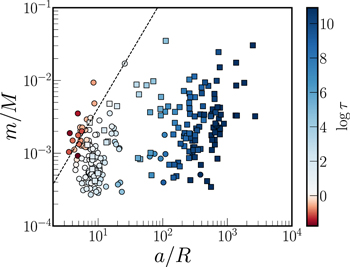
Figure 1. Planet-to-star mass ratio (m/M) and orbital distance to stellar radius ratio (a/R) for stars with giant planets. Circles represent transiting planets, and squares represent Doppler-detected planets. The color conveys the value of  , where τ is the ratio of the theoretical spin-up time to the estimated main-sequence age. The blue (red) points depict systems for which we expect weak (strong) tidal spin-up. The white points are near the boundary of τ = 1.5 chosen to separate HJs and control Jupiters (CJ). This boundary is nearly equivalent to a critical value of 1.6 × 10⁹ for η, which is shown with the dotted line.
Download figure:
Standard image High-resolution imageMuch of the subsequent analysis was based on the separation of the samples into two groups, one of which is theoretically expected to have experienced significant tidal spin-up, and the other of which involves planets that are not massive enough or close enough to the star to expect much tidal spin-up. To divide the sample, we chose a critical value τc = 1.5 because it corresponds to a nominal case in which the theoretical spin-up timescale is 10 Gyr for a Jupiter-mass planet in a 5-day orbit around a Sun-like star with a rotation period of 25 days and  at a corresponding age of 4.5 Gyr. For reference, this nominal case also has η = 1.6 × 10⁹.
We refer to systems with τ < τc as HJs and the giant-planet systems with τ > τc as CJ. This definition led to a sample of 32 HJs and 208 CJs. Of the CJs, 90 are transiting planets and 118 were detected with the Doppler method. 5 These population numbers are also given in Table 2. There was no need to divide up the CKS systems because they all have τ ≫ τc, given the low masses of the planets.
Table 2. Planet Samples
| Characteristic | HJ | CJ | CKS |
|---|---|---|---|
| Total number | 32 | 208 | 283 |
| Transit discoveries | 32 | 90 | 283 |
| Doppler discoveries | 0 | 118 | 0 |
| Photometric rotation periods | 19 | 24 | 67 |
| Spectroscopic rotation periods | 0 | 35 | 0 |
Note. Characteristics of the HJ and CJ samples. Notably, all of the HJs and CKS planets were detected in transit surveys, while the CJS contain a mixture of transiting and Doppler-detected planets.
Download table as: ASCIITypeset image
Figure 2 shows the distribution of masses and orbital periods of the planets in our samples. The CKS period distribution overlaps with the HJ and CJ samples, but the masses are all substantially lower. 6 Thus, we have two control samples to compare to the HJ sample: the CJs have similar masses and wider orbits, while the CKS planets have lower masses and a broader range of orbital distances.
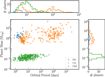
Figure 2. Planet mass vs. orbital period for the HJs, CJs, and CKS planets. Circles represent transit-discovered planets, and squares represent Doppler-discovered planets.
Download figure:
Standard image High-resolution image2.5. Comparison of Spectroscopic Parameters
Ideally, the control samples would consist of stars with the same distribution of masses, compositions, and ages as the HJ hosts. We should not expect them to align perfectly because the stars are drawn from different surveys and because of astrophysical correlations between stellar and planetary properties (such as the well-known tendency for giant-planet hosts to have higher than average metallicity). Nevertheless, we can check for any major mismatches that would invalidate our comparisons.
A concern with the CJs is that more than half of the sample is drawn from Doppler surveys, whereas all of the HJs were identified in transit surveys. Transit and Doppler surveys are subject to different selection effects favoring the detection of planets around different types of stars. We must therefore make sure that despite these different selection effects, the CJ hosts have spectroscopic properties similar to those of the HJ hosts. Furthermore, the orbital inclinations of the transiting planets are all very close to 90°, while those of the Doppler planets have a much broader range of inclinations. This has two relevant consequences. First, the masses of the Doppler planets are formally unknown; only the minimum possible mass ( ) can be measured. To account for this ambiguity, whenever the planet mass was needed, we divided
  by π/4, the average value of
  for random orientations.
7
Second, to the extent that the inclination of the stellar spin axis is correlated with the orbital inclination, the transiting planets would have a different distribution of
for random orientations.
7
Second, to the extent that the inclination of the stellar spin axis is correlated with the orbital inclination, the transiting planets would have a different distribution of  than the Doppler planets even if they have the same distribution of rotation velocities. We return to address this complication in Sections 3 and 4.
The CKS sample of small-planet host stars consists entirely of transiting planets, so it does not suffer from the problems just described for the giant-planet sample. Here, a concern is that giant-planet hosts are known to be more metal rich as a whole than the hosts of smaller planets (Gonzalez 1997; Fischer & Valenti 2005; Santos et al. 2005; Petigura et al. 2018). Any astrophysical correlation between metallicity and rotation would be a confounding factor in the comparison between the CKS stars and the giant-planet hosts.
Figures 3 and 4 compare the spectroscopic parameters and isochrone-fitting results of the HJ, CJ, and CKS samples. Our lower and upper limits on  and [Fe/H] were determined through inspection of these plots; the gray points are the stars that were rejected because their parameters are too different from those of the majority of the stars. The metallicity effect is apparent in the upper right panel of Figure 4. There is also a tendency for the CKS stars to be assigned smaller radii and older ages than the HJ hosts of a given mass, evident in the lower left panel of Figure 4. This could be related to the finding by Hamer & Schlaufman (2019) that the hosts of HJs are kinematically younger (i.e., have a lower velocity dispersion) than similar stars without hot JHs.
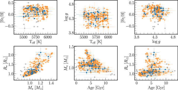
Figure 3. Comparison of the spectroscopic and physical properties of the host stars of HJs (blue) and CJs (orange). Circles are for transit detections, and squares are for Doppler detections. Note the absence of HJs at low metallicities. The gray points are those that were rejected for being outside the designated metallicity range.
Download figure:
Standard image High-resolution image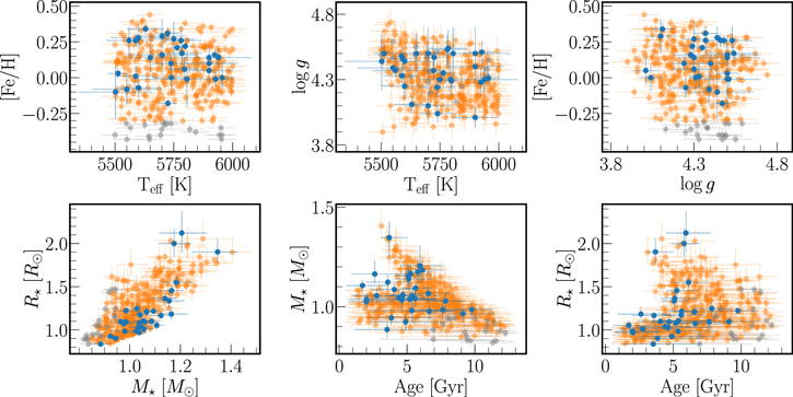
Figure 4. Comparison of the spectroscopic and physical properties of the host stars of HJs (blue) and CKS planets (orange). Circles are for transit detections and squares are for Doppler detections. The gray points are those that were rejected for being outside the designated metallicity range. In addition to the absence of HJs at low metallicities, note that the HJs tend to be found around lower-mass higher-gravity younger stars.
Download figure:
Standard image High-resolution imageIn addition to these patterns, the samples seem to span approximately the same range of parameters. We employed a two-sided Kolmogorov–Smirnov (KS) test for each spectroscopic parameter to try and rule out the null hypothesis that the parameter values for the HJ hosts and control stars are drawn from the same distribution. The p-values, given in Table 3, all exceed 0.05.
Table 3. p-values of Two-sample KS Tests for the Distributions of Spectroscopic Parameters Relative to the HJ Sample
| Control Sample | Teff | Metallicity |

|
|---|---|---|---|
| CJ | 0.36 | 0.79 | 0.14 |
| CKS | 0.43 | 0.07 | 0.08 |
Download table as: ASCIITypeset image
3. Comparison of Rotation Parameters
We gathered all of the available information about the rotation properties of the stars. We found  measurements for all the stars in the literature. We decided to regard as upper limits all the cases in which
  was reported to be lower than 2 km s−1, out of concern about systematic errors.
We also searched the literature for stellar rotation periods measured from either time-series broadband photometry, or spectroscopic monitoring of emission-line fluxes. We did not accept rotation periods based on measurements of  and the assumption
  , nor did we use estimated rotation periods based only on the overall level of chromospheric activity. Needless to say, we did not use rotation periods based on gyrochronology either. Using these criteria, we found rotation periods for 78 stars (19 HJs and 59 CJs). We also found measurements of the photometric rotation periods for 68 of the CKS stars in the catalog of Mazeh et al. (2015).
8
We adopted the period uncertainties from the literature and assumed an uncertainty of 20% when the uncertainty was not clearly documented.
, nor did we use estimated rotation periods based only on the overall level of chromospheric activity. Needless to say, we did not use rotation periods based on gyrochronology either. Using these criteria, we found rotation periods for 78 stars (19 HJs and 59 CJs). We also found measurements of the photometric rotation periods for 68 of the CKS stars in the catalog of Mazeh et al. (2015).
8
We adopted the period uncertainties from the literature and assumed an uncertainty of 20% when the uncertainty was not clearly documented.
3.1. Projected Rotation Velocity
We compared the  distributions of our samples to see if the HJ hosts are rotating systematically faster, given their ages. However, any observed differences in the
  distributions could be due to differences in
  as well as rotation velocity. It seems safe to assume that the hosts of all the Doppler-detected planets are nearly randomly oriented, in which case any systematic differences in
  between large populations of stars can be interpreted as differences in rotation velocity.
The situation is more complicated for the hosts of transit-detected planets. Transiting planets all have orbital inclinations near 90°. Thus, if the stellar rotation axes are aligned with the orbital axes, the stars with transiting planets would have systematically higher  values than stars with Doppler planets, even if their distributions of rotation velocities were the same. This complicates our comparison between HJs and CJs, because the HJs are mainly composed of transit-detected planets, while the CJs are a more even mixture of transit and Doppler discoveries.
Previous measurements have established that Sun-like stars with HJs generally have low obliquities implying  (see, e.g., Winn et al. 2010; Albrecht et al. 2012). The obliquity distribution of stars with smaller or wider-orbiting planets is less well known. There is statistical evidence that the Sun-like stars in the Kepler sample (including the stars in our CKS sample) have low obliquities, based on the distribution of photometric variability amplitudes (Mazeh et al. 2015) as well as tests involving
  data (Winn et al. 2017). These results suggest that the
  distributions of the transiting HJs and the CKS stars are similar, and it is safe to interpret any systematic differences in
  as differences in rotation velocity.
However, for the CJs, things may be different. There are known cases of Sun-like stars with high obliquities relative to wider-orbiting giant planets, such as WASP-17b, WASP-130b, WASP-134b, and HATS-18b (Smith et al. 2013; Brahm et al. 2016; Hellier et al. 2017; Anderson et al. 2018, respectively). Hence, the mean value of  in the sample of transiting HJs may be higher than that of the transiting CJs, confounding the interpretation of the differences in the
  distributions.
We dealt with this issue by considering two limiting cases. In the first case, the transiting HJs and CJs were both assumed to have low obliquities and  . In the second case, which we consider rather extreme, the transiting HJ hosts were assumed to have zero obliquity (
 ), and the transiting CJ hosts were also assumed to be randomly oriented (
 on average).
Figure 5 compares the rotation-velocity distributions of the HJs and control stars. In all of the panels, the plotted velocity for the Doppler planets is  divided by π/4. The top left panel represents the first case described above: for all the transiting planets, the plotted velocity is
  . The top right panel represents the second case: the plotted velocity is
  for the transiting HJs, and
  for all CJs. The bottom right panel compares the HJ and CKS samples; in this case, the plotted velocity is
  for all the transiting planets. Finally, the bottom left panel of Figure 5 compares the HJs and CJs after excluding the Doppler planets; thus, it is a transit-to-transit comparison. For this figure, the plotted velocity is
  for both HJs and CJs.
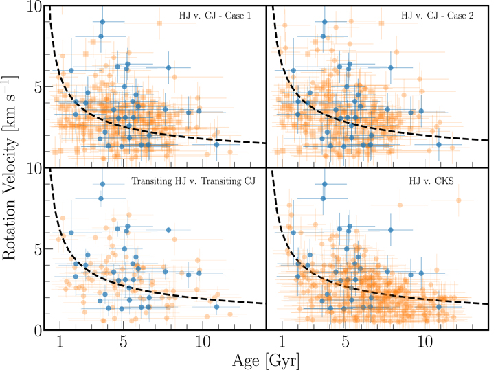
Figure 5. Rotation velocity as a function of isochrone age. Blue points are for HJ hosts, and orange points are for control stars. Squares depict Doppler-discovered planets, and circles depict transit-discovered planets. The dashed line is the best fit to the control stars using Equation (5). The plotted “rotation velocity” is  for the transiting HJs,
  for the CKS stars, and
  for the Doppler-detected planets. For the transiting CJs, two different cases are considered. Top left.—Case 1, assuming transiting CJs have
  . Top right.—HJs vs. CJs, assuming the CJ hosts are randomly oriented (
 ). Bottom left.—Transiting HJs and CJs only assuming CJ hosts are randomly oriented. Bottom right.—HJs vs. CKS stars. The two outliers are Kepler-1505 and Kepler-461, both of which also have unusually high variability amplitudes.
Download figure:
Standard image High-resolution imageIn all of these cases, the HJ hosts appear to have systematically faster rotation than the CJ hosts. To quantify the differences, we fitted a Skumanich (1972) law,

to the control-star data. The only free parameter was v0. The HJ data fall mainly above the best-fitting curves (i.e., the blue points are mainly above the dashed lines). We defined a sum-of-residuals statistic,

where  is the observed value,
  is the calculated value using the best-fitting function (Equation (5)), and the sum runs over all the data points. To estimate the probability that high S values are the result of random fluctuations, we used a Monte Carlo procedure. In each Monte Carlo realization of the data, we randomly drew (with replacement) a subset of stars from the entire sample of stars—both HJs and control stars—to play the role of fictitious HJs. We performed 106 such simulations and asked how often the S value of the simulated data was at least as large as the S value of the real data. The resulting p-values, given in the first column of Table 4, are lower than 0.004 regardless of the control sample or assumed obliquity distribution. These low p-values confirm the visual impression that the HJ hosts tend to rotate faster at all ages.
Table 4. p-values of Two-sample KS Tests for the Distributions of Rotation Parameters Relative to the HJ Sample
| Control Sample |
 , Case 1 , Case 1 |
 , Case 2 , Case 2 | Prot |
|---|---|---|---|
| CJ | 2 × 10⁻⁴ | 4 × 10⁻³ | ≲10−6 |
| CKS | 3 × 10⁻⁴ | 3 × 10⁻⁴ | 8 × 10⁻⁵ |
Note. Case 1 assumes the transiting CJs have  , while Case 2 assumes they have
  .
.
Download table as: ASCIITypeset image
Another way to see the evidence for spin-up is to examine the  distribution as a function of effective temperature rather than isochrone age, as shown in Figure 6. This comparison has the advantage of being independent of uncertainties in the isochrone ages. At any given effective temperature, the HJ hosts have systematically higher
  values than the stars in the control samples. Following the example of Louden et al. (2021), we fitted a quadratic function to the relation between
  and Teff for each control sample (dashed curves, in Figure 6). The residual test discussed above yields a p-value ≲ 10−6 for the comparison with CKS stars. For the comparison with the CJs, the p-value is 5.0 × 10⁻⁵ and 3.4 × 10⁻³ for Cases 1 and 2, respectively.
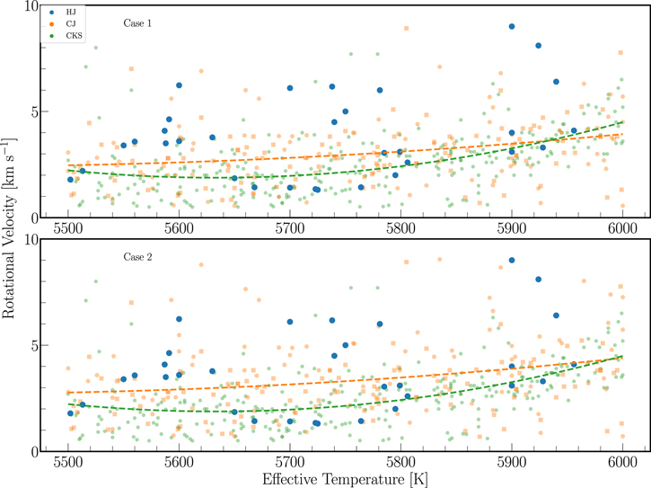
Figure 6. Rotation velocity as a function of effective temperature, for HJ hosts (blue points), CJs (orange points), and CKS stars (green points). As in Figure 5, the plotted velocity is  for the transiting HJs and CKS stars, and
  for the Doppler planets. Two cases are considered for the transiting CJs. Top.—Case 1, in which the plotted velocity is
  for CJ transit discoveries. Bottom.—Case 2, in which it is
  . The dashed curves are quadratic functions fitted to the control-star data.
Download figure:
Standard image High-resolution image3.2. Rotation Period
By comparing rotation periods rather than projected rotation velocities, we avoid the complications due to the unknown obliquity distributions. The penalty is, however, that rotation periods have only been measured for a subset the stars in our sample. This reduces the sample sizes and the statistical power of any comparisons. Furthermore, the stars with measured rotation periods are not necessarily representative of the whole sample. Rotation periods are easier to measure when the amplitude of variability is high, which in turn is associated with youth, rapid rotation, and high inclination. While these biases should apply to all of the samples and cancel out to some degree, there may be residual biases that are difficult to quantify.
These limitations notwithstanding, Figure 7 shows rotation period versus isochrone age for the HJ, CJ, and CKS samples. Compared to the control samples, the HJ hosts have systematically shorter periods and more rapid rotation. The left panel, in which the CJs are the control sample, shows that Doppler-detected planets tend to have longer periods than transit-detected planets. This could be due at least in part to a bias against rapid rotators in the Doppler surveys. However, the right panel, in which the CKS stars are the control sample, does not suffer from that particular bias and also shows the HJ hosts to be rotating faster.
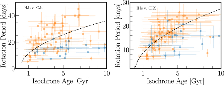
Figure 7. Rotation period vs. isochrone age for the HJs (blue) and the control sample (orange), which is the CJ sample in the left panel and the CKS sample in the right panel. Squares are for Doppler-detected planets and circles are for transit-detected planets. The dashed curves are functions with the form of Equation (7) fitted to the control sample.
Download figure:
Standard image High-resolution imageAs before, we quantified the differences by fitting the control data to a Skumanich-like law, 9

where P0 is a free parameter, and then calculated the period-based sum-of-residuals S for the HJ host stars. In this case, the HJ hosts have a negative value of S, i.e., they have shorter rotation periods than would be predicted from the fit to the control-star data. The p-values, given in Table 4, are low enough for the pattern to be deemed highly significant.
3.3. Rotation versus Tidal Spin-up Parameter
The preceding tests convinced us that the HJ hosts do indeed rotate systematically faster than the control stars, whether the measure of rotation is the projected rotation velocity or the rotation period, or whether the comparison is performed as a function of isochrone age or effective temperature. To search for evidence that tidal spin-up is the reason for the excess rotation, we tested for a correlation between rotation and the theoretically expected degree of tidal spin-up, quantified by our τ parameter. As a reminder, τ is the ratio of the tidal spin-up timescale in the theory of Lai (2012) and the isochrone age, with lower values corresponding to a higher expectation for tidal spin-up.
Figure 8 reproduces the data that were shown in Figures 5 and 7, but in this case, the color of each point conveys the calculated value of τ, with darker points representing systems where tidal spin-up should be most significant. As expected, the darker points tend to be associated with higher rotation velocities and shorter rotation periods. Figure 9 shows more directly the association between excess rotation and τ. For this figure, the excess rotation was defined as the difference between the observed value of rotation velocity or period, and the calculated value based on the Skumanich-like function fitted to the control-star data. The plots are restricted to the range of τ between 0.1 and 1000, where we might expect to see a correlation (this excludes many of the CKS systems for which τ ≫ 1000).
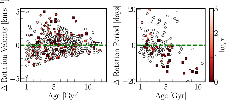
Figure 8. Case 1 deviation of rotation velocity and rotation period as a function of isochrone age, color-coded according to τ, the tidal spin-up timescale divided by the isochrone age. Green fiducial line indicates  . The data from all the samples are plotted (HJ, CJ, and CKS). For clarity in this particular figure, the squares represent the HJ planets and circles illustrate the CJs. Lower τ values, indicating strong tides, show higher excess velocity from the Skumanich law.
Download figure:
Standard image High-resolution image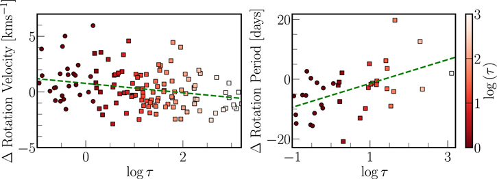
Figure 9. Projected rotation velocity (left) and rotation period (right) as a function of τ, the tidal spin-up timescale divided by the isochrone age. Stars with lower values of τ show faster rotation velocities and shorter rotation periods. Squares represent Doppler-detected planets and circles depict transit-detected planets.
Download figure:
Standard image High-resolution imageThe excess rotation and the parameter τ are indeed correlated, as confirmed through least-squares fitting. Between  and τ there is a shallow but significant negative correlation: Table 5 gives the results of the Pearson and Spearman tests.
10
and τ there is a shallow but significant negative correlation: Table 5 gives the results of the Pearson and Spearman tests.
10
Table 5. Correlation Coefficients (r) and p-values between τ and Rotation Parameters
| Parameter | Pearson | Spearman | ||
|---|---|---|---|---|
| r | p | r | p | |

| −0.26 | 2.6 × 10⁻³ | −0.24 | 6.0 × 10⁻³ |
| Prot | + 0.53 | 4.6 × 10⁻⁴ | + 0.50 | 1.0 × 10⁻³ |
Download table as: ASCIITypeset image
4. Summary and Discussion
We investigated the evidence for tidal spin-up in HJ systems by comparing the rotation velocities and spin periods of Sun-like stars with a wide range of ages and planet parameters. The stars that are theoretically expected to have been most susceptible to tidal spin-up–those with close-orbiting giant planets—are indeed rotating faster than comparable stars with other types of planets. By preparing appropriate samples and performing simple comparisons, our approach was intended to be more empirical and less model dependent than the complementary studies of Jackson et al. (2009), Hansen (2010), Ferraz-Mello et al. (2015), Penev et al. (2018), Barker (2020), and Anderson et al. (2021), who have modeled secular evolution in the context of specific tidal models. In our study, the only input from theory was in the definition of the dimensionless parameters η and τ that quantify the expected degree of tidal effects.
A limitation of our study is that although we did perform the isochrone analysis for all the stars in the same manner, the input data were all drawn from the literature, which means that the spectroscopic and rotation parameters were derived by different authors using different techniques. The CKS parameters were homogeneously derived, but the giant-planet parameters come from heterogeneous sources. Another limitation is that our samples contain planets discovered in surveys with different selection biases. All of the HJs and CKS planets were discovered with the transit technique, while the CJs consist of a mixture of transit-detected and Doppler-detected planets. The Doppler surveys do not find many planets around young and rapidly rotating stars because of the difficulty of achieving good precision when the spectra have broad lines with time-variable distortions. There is also the issue that the distribution of  is different for the Doppler- and transit-detected systems and may also vary with the planet properties. We dealt with these issues by performing additional tests with different subsamples (e.g., only transiting planets) and under different assumptions about the
  distribution (Cases 1 and 2). These robustness tests led to the same conclusion—the HJ hosts spin faster than the control stars—but, naturally, with reduced statistical significance.
Our results, based on larger samples and more controlled comparisons, reinforce earlier evidence presented by Brown (2014) and Maxted et al. (2015) that close-orbiting giant planets are able to influence the rotation rates of their host stars while they are on the main sequence. In addition, measurements of rotation rates, another line of evidence that pointed to the same conclusion, were presented by Poppenhaeger & Wolk (2014), who found several HJ hosts to be more chromospherically active than their binary companions on wide orbits.
An immediate implication is that gyrochronology is unreliable for stars with HJs, in agreement with previous empirical findings by Brown (2014) and Maxted et al. (2015) and theoretical work by Ferraz-Mello et al. (2016). The spin history of these stars is abnormal, invalidating the usual relations between mass, age, and rotation velocity. Another implication is that HJ orbits decay significantly during the main-sequence lifetime of the star; the angular momentum that is transferred to the star’s rotation must come at the expense of the planet’s orbit. The same conclusion was reached by Hamer & Schlaufman (2019), who showed that Sun-like stars with HJs are “kinematically young,” i.e., they have a lower Galactic velocity dispersion than similar stars without HJs. They took the low occurrence of HJs around kinematically older stars to be evidence for tidal destruction on Gyr timescales. Our work supports this conclusion not only by identifying excess rotation of the HJ hosts, but also in observing the tendency for HJ hosts to have younger isochrone ages (Figures 3 and 4).
The evidence for tidal transfer of angular momentum also suggests that HJs can affect the spin direction of the star and that obliquity damping can occur while the star is on the main sequence. In this sense, our results complement earlier work showing that Sun-like stars with HJs tend to have low obliquities, while stars that are more massive or that have planets on wider orbits are sometimes observed to have high obliquities (Winn et al. 2010; Albrecht et al. 2012). Theorists have indicated that the timescales for spin-up (and the associated orbital decay) and obliquity alteration need not always be the same (Lai 2012; Barker 2020), but for Sun-like stars with HJs, both effects do appear to be significant.
It would be interesting to extend this study to other types of stars, both less and more massive than the Sun-like stars considered here, because the mechanisms for tidal dissipation may be quite different. For massive stars, at this stage the main difficulty would be constructing suitable control samples. There are plenty of F stars known to have HJs, but not as many F stars with giant planets on wide orbits or considerably smaller planets. For the extension to low-mass stars, one problem is that HJs are themselves rare around low-mass stars. Moreover, our understanding of the rotational evolution of low-mass stars is limited in comparison to our understanding of Sun-like stars. The situation will probably improve as the NASA TESS mission (Ricker et al. 2014) continues to find planets and measure rotation periods with ever greater sensitivity (see, e.g., Martins et al. 2020), and after the PLATO mission commences (Rauer et al. 2014).
We thank Kaloyen Penev for helpful discussions. This work was supported by NASA grant ATP 80NSSC18K1009. K.R.A. is supported by a Lyman Spitzer, Jr. Postdoctoral Fellowship at Princeton University.
Software: Astropy (Price-Whelan et al. 2018), Jupyter Notebooks (Kluyver et al. 2016), Matplotlib (Hunter 2007), NumPy (Van Der Walt et al. 2011; Harris et al. 2020), Pandas (pandas development team 2020), SciPy (Virtanen et al. 2020), VizieR (Ochsenbein et al. 2000).
Footnotes
- 2
- 3
Anderson et al. (2021) used broadband photometry from 2MASS, WISE, and Gaia Data Release 2. We chose to fit only the Gaia photometry.
- 4
According to this definition,
 , where Q is the (unmodified) tidal quality factor, and k2 is the tidal Love number.
 - 5
Although the results described this paper were obtained with the choice τc = 1.5, we confirmed that none of our conclusions hinge on this exact choice. Qualitatively similar results are obtained for any value of τc of the same order of magnitude. We also obtained similar results when dividing the samples according to a critical value of η instead of τ.
- 6
We calculated the expected planet masses based on their measured radii, using Equation (1) of Wolfgang et al. (2016).
- 7
In fact, for a sample of Doppler-detected planets,
because the sample is deficient in low-inclination systems, but we neglected this minor effect. - 8
We only considered the photometric rotation periods that were considered most reliable by McQuillan et al. (2014); in their terminology, the “weight” exceeds 0.25. We also decided to omit Kepler-1563 because the reported rotation period of 46 days is nearly twice as long as any of the other rotation periods in the sample. Measurements of such long periods are probably subject to additional uncertainty because the Kepler data segments (“quarters”) span only 90 days.
- 9
- 10
The Pearson correlation coefficient is the covariance of two variables divided by the product of their standard deviations. The Spearman rank correlation coefficient is the Pearson correlation coefficient between the rank-ordered values of the two variables.

