Abstract
We investigate the spatial distribution of the satellites of isolated host galaxies in the IllustrisTNG100 simulation. In agreement with a previous, similar analysis of the Illustris-1 simulation, the satellites are typically poor tracers of the mean host mass density. Unlike the Illustris-1 satellites, here the spatial distribution of the complete satellite sample is well fitted by an NFW profile; however, the concentration is a factor of ∼2 lower than that of the mean host mass density. The spatial distributions of the brightest 50% and faintest 50% of the satellites are also well fitted by NFW profiles, but the concentrations differ by a factor of ∼2. When the sample is subdivided by host color and luminosity, the number density profiles for blue satellites generally fall below the mean host mass density profiles, while the number density profiles for red satellites generally rise above the mean host mass density profiles. These opposite, systematic offsets combine to yield a moderately good agreement between the mean mass density profile of the brightest blue hosts and the corresponding number density profile of their satellites. Lastly, we subdivide the satellites according to the redshifts at which they joined their hosts. From this, we find that neither the oldest one-third of the satellites nor the youngest one-third of the satellites faithfully trace the mean host mass density.
Original content from this work may be used under the terms of the Creative Commons Attribution 4.0 licence. Any further distribution of this work must maintain attribution to the author(s) and the title of the work, journal citation and DOI.
1. Introduction
Dark matter halos in Λ cold dark matter (ΛCDM) simulations are known to follow a spherically averaged characteristic density profile, often parameterized as a Navarro−Frenk−White (NFW; Navarro et al. 1996) profile:
Here ρcrit is the critical density for closure of the universe, δc is a dimensionless characteristic density, and rs is a scale radius, defined as the ratio of the virial radius, r200, and the concentration parameter, c: rs ≡ r200/c. The characteristic density, δc , and the concentration parameter are related through
The NFW profile was first identified in N-body (i.e., dark-matter-only) simulations. While the implementation of baryonic physics in ΛCDM simulations results in dark matter halos that, in three dimensions, are rounder and more oblate than the halos in N-body simulations (see, e.g., Chua et al. 2019), the spherically averaged density profiles of the dark matter halos in these cosmological hydrodynamical simulations still follow NFW density profiles at all but the smallest radii (see, e.g., Brainerd 2018).
The shapes of the density profiles of dark matter halos in the observed universe, as well as whether or not they follow NFW-like profiles, are important tests of ΛCDM. Given the invisible nature of the dark matter, some type of luminous tracer of the dark matter halos of observed galaxies is, of course, necessary in order to directly constrain their mass density profiles. Satellite galaxies, orbiting about bright, central “host” galaxies, could potentially serve as such tracers. However, the degree to which satellite galaxies faithfully trace the underlying mass distributions of their host galaxies is unclear.
Budzynski et al. (2012) found that the radial number density profiles of the satellites in observed groups and clusters of galaxies were well fitted by NFW profiles. Compared to predictions from ΛCDM, however, the concentration found by Budzynski et al. (2012) was a factor of ∼2 lower than expected. In another study of observed galaxy clusters, Wang et al. (2018) compared the locations of the satellites to the weak-lensing-derived cluster mass distribution. From this, Wang et al. (2018) found that the satellite number density traced the mass density well, with both the satellite number density and the mass density being well fitted by an NFW profile.
In a study of the locations of the satellites of massive red host galaxies, Tal et al. (2012) found that, at large distances from their hosts, the radial number density profile of the satellite galaxies could be fitted by an NFW profile. Close to the central galaxy, however, Tal et al. (2012) found that the satellite number density exceeded the expectations of an NFW profile. Similarly, Watson et al. (2012) investigated the small-scale clustering of satellite galaxies in the Sloan Digital Sky Survey (SDSS; York et al. 2000) and found that while the spatial distribution of satellites with Mr > −19.5 was fitted well by an NFW profile, the spatial distribution of brighter satellites had a slope that was steeper than expected from an NFW profile. In another study of SDSS galaxies, Piscionere et al. (2015) found that the distribution of their most luminous satellites (Mr <−20) showed a steep upturn at small distances from the host galaxy. In a study of isolated SDSS host galaxies, Wang et al. (2014) found that the spatial distribution of the satellites of high-mass hosts (M* > 1011 M⊙) was less concentrated than would be expected for the hosts’ dark matter halos, but that the satellites of low-mass hosts followed the expected dark matter distribution. In contrast, Guo et al. (2012) found that the spatial distribution of the satellites of isolated SDSS host galaxies agreed with an NFW profile, with small exceptions at small radii or low luminosity.
Mixed conclusions regarding the degree to which satellite galaxies in ΛCDM simulations trace the surrounding mass distribution have also been reached. Gao et al. (2004) applied a semianalytic galaxy formation model (SAM) to 10 high-resolution resimulations of cluster-mass halos and found that the radial distribution of luminous galaxies closely followed that of the dark matter. Using a numerical hydrodynamical simulation, Nagai & Kravtsov (2005) studied the distribution of the satellites in galaxy clusters and concluded that the satellite distribution was less concentrated than the dark matter, particularly in the inner regions of the clusters. Sales et al. (2007) applied a SAM to the Millennium simulation (Springel et al. 2005) and found that the spatial distribution of the satellites of bright, isolated host galaxies was well fitted by an NFW profile that was only slightly less concentrated than the best-fitting NFW profile for the host galaxies’ dark matter halos. Using a SAM applied to the Millennium and Millennium II (Boylan-Kolchin et al. 2009) simulations, Wang et al. (2014) found that the satellite distribution around isolated host galaxies traced the hosts’ dark matter halos well. Similarly, Guo et al. (2013) found that the radial distributions of the satellites of isolated host galaxies in the Millennium and Millennium II simulations could be fitted by NFW profiles. However, when Guo et al. (2013) subdivided their samples by color, they found that, because the simulation produced too few blue satellite galaxies compared to the observed universe, the shapes of the number density profiles of their simulated and observed galaxies were no longer similar to each other.
More recently Ágústsson & Brainerd (2018) investigated the spatial distributions of satellite galaxies that were selected from a mock redshift survey of the Millennium simulation. Using satellites that were obtained using redshift space proximity criteria, Ágústsson & Brainerd (2018) found that the locations of the satellites of isolated red host galaxies traced the hosts’ dark matter halos well. In the case of isolated blue host galaxies, however, Ágústsson & Brainerd (2018) found that the concentration of the satellite distribution was roughly twice that of the hosts’ dark matter halos. In addition, the locations of satellite galaxies in the Illustris-1 simulation (Vogelsberger et al. 2014; Nelson et al. 2015) were investigated by Ye et al. (2017) and Brainerd (2018). Ye et al. (2017) focused on halos with virial masses in the range 1012 h−1 M⊙ < M200 < 1014 h−1 M⊙, while Brainerd (2018) focused on isolated host galaxies with median virial masses ∼1012 M⊙. Ye et al. (2017) found that the locations of the satellite galaxies traced the dark matter halos well at large radii, but for radii ≲0.4r200 the dark matter distribution was traced well by only those satellites with a high satellite-to-host mass ratio. Brainerd (2018) found that the satellite number density profile was inconsistent with an NFW profile and, for small host−satellite separations, the satellite number density profile increased steeply.
The disparate conclusions that have been reached regarding the relationship between satellite number density profiles and host mass density profiles may indicate that the sample selection criteria and/or the models in the simulations influence the degree to which satellite galaxies are found to trace the local mass distribution. Here we revisit the question of whether or not the locations of satellite galaxies in a ΛCDM simulation faithfully trace the dark matter distribution that surrounds isolated host galaxies. Using a hydrodynamical simulation that reproduces the red–blue color bimodality of galaxies in the observed universe, we compute the locations of the satellites as a function of the colors and luminosities of the host and satellite galaxies. The paper is organized as follows. The selection of the host galaxies and their satellites, as well as the properties of the sample, is described in Section 2. Normalized satellite number density profiles are compared to normalized mass density profiles of the host galaxies in Section 3. A summary and discussion of the results are presented in Section 4, and our main conclusions are presented in Section 5.
2. Host−Satellite Sample
Our host−satellite sample is drawn from the z = 0 snapshot of the IllustrisTNG100 simulation. The IllustrisTNG project (Marinacci et al. 2018; Naiman et al. 2018; Nelson et al. 2018, 2019; Pillepich et al. 2018a; Springel et al. 2018) is a suite of ΛCDM magnetohydrodynamical simulations, all of which are publicly available. The simulations adopted a Planck Collaboration (2016) cosmology with the following parameter values: ΩΛ,0 = 0.6911, Ωm,0 = 0.3089, Ωb,0 = 0.0486, σ8 = 0.8159, ns = 0.9667, and h = 0.6774. Here the TNG100 simulation was chosen because it offers good resolution of relatively faint satellite galaxies (Mr ∼ −14.5). In addition, the number of dark matter particles (18203), the number of gas particles at the start of the simulation (18203), the comoving volume of the simulation (753 h−3 Mpc3), and the initial conditions are identical to those of the Illustris-1 simulation. This makes comparison between our results and those of Brainerd (2018) straightforward. Excluding subhalos that are flagged as being noncosmological in origin, there are ∼60,000 (Mr < −14.5) luminous galaxies in the TNG100 simulation at z = 0.
Key differences between the original Illustris simulations and the IllustrisTNG simulations are the ways in which active galactic nucleus (AGN) feedback, galactic winds, and the growth of supermassive black holes were treated (see Weinberger et al. 2017; Pillepich et al. 2018b). These changes successfully addressed a shortcoming of the original Illustris simulations: the lack of a clear red–blue color bimodality for present-day galaxies. Unlike Illustris-1, the TNG100 simulation shows a red–blue color bimodality for present-day galaxies that is comparable to the color distribution of low-redshift galaxies in the observed universe. For rest-frame Sloan (g − r) color, the division between “red” and “blue” galaxies occurs at (g − r) = 0.65 for TNG100 galaxies at redshift z = 0 (see Nelson et al. 2018).
In order to compare our results from TNG100 to those obtained from Illustris-1, we adopt the same 3D selection criteria as Brainerd (2018). Each host galaxy must have an absolute magnitude brighter than −20.5 in the r band, be located at the center of its friends-of-friends halo, and be at least 2 mag brighter than any other galaxy within a distance of 1 h−1 Mpc. The last of these criteria ensures that the host galaxies are “isolated” and, in general, the criteria we have adopted will select host−satellite systems that are more isolated than the Milky Way or M31. Although isolation ensures that the hosts are at the centers of the potentials and that the satellites do not experience significant gravitational effects due to other nearby, large galaxies, isolation also results in the selection of bright central galaxies that have relatively few neighboring galaxies compared to nonisolated bright central galaxies. For the bright, central galaxies that satisfy the above criteria, all galaxies with Mr < −14.5 that are within 2r200 of the bright galaxy are defined to be satellites. To ultimately qualify as being a “host” in our sample, the bright central galaxy must have at least one satellite within the virial radius.
The galaxy magnitudes that we use here are the sum of the intrinsic emission of all bound star particles, as described in Pillepich et al. (2018a), and the effects of dust obscuration are not included. Following Nelson et al. (2018), we use the (g − r) colors of the hosts and satellites to split our sample into “red” and “blue” galaxies, where red galaxies are those with (g − r) ≥ 0.65 and blue galaxies are those with (g − r) <0.65. We have verified that our results below are not overly sensitive to the precise value of (g − r) color that is used to separate the galaxies according to color.
Table 1 lists various properties of the host galaxies as a function of host color. In order, these are number of hosts, median r-band absolute magnitude, median number of satellites within the virial radius, maximum number of satellites in a system, median stellar mass, median virial mass, minimum virial mass, maximum virial mass, median virial radius, minimum virial radius, and maximum virial radius. From Table 1, although red and blue hosts are similarly bright, red hosts have stellar masses and virial masses that are systematically larger than those of blue hosts. In addition, red hosts typically have more satellites within their virial radii than do blue hosts. From Table 1, the selection criteria result in the inclusion of a handful of group- and cluster-sized objects. This is also true of the host−satellite samples in Brainerd (2018) and Sales et al. (2007) (which were obtained using the same criteria as we adopt here) and does not affect our conclusions below. Brainerd (2018) investigated the effects of inclusion of these larger systems and found that they did not significantly affect the conclusions regarding the degree to which the satellite distributions differed from the host mass distributions.
Table 1. Host Galaxy Properties
| Property | Red Hosts | Blue Hosts |
|---|---|---|
| Number | 286 | 461 |

| −21.7 | −21.5 |

| 2 | 1 |

| 145 | 230 |

| 5.65 × 10¹⁰ M⊙ | 2.39 × 10¹⁰ M⊙ |

| 2.79 × 10¹² M⊙ | 1.05 × 10¹² M⊙ |

| 1.20 × 10¹² M⊙ | 5.17 × 10¹¹ M⊙ |

| 2.13 × 10¹⁴ M⊙ | 1.71 × 10¹⁴ M⊙ |

| 297 kpc | 214 kpc |

| 197 kpc | 149 kpc |

| 1260 kpc | 1170 kpc |
Download table as: ASCIITypeset image
The top panels of Figure 1 show the (g − r) color distributions of the host and satellite galaxies, from which it is clear that the majority of the hosts are blue and the majority of the satellites are red. Figure 1(c) shows the fraction of satellites inside the virial radius that are red in color, computed as a function of host color. From Figure 1(c), a clear color–color correlation exists for the host galaxies and their satellites, with blue hosts having a smaller fraction of satellites that are red in color and ≳50% of the satellites of red hosts being red in color.
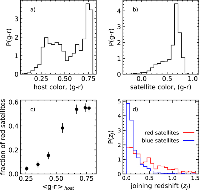
Figure 1. Properties of the host−satellite sample. (a) Probability distribution of host (g − r) colors. (b) Probability distribution of satellite (g − r) colors. (c) Fraction of satellites within the virial radius that are red in color, computed as a function of host color. (d) Probability distribution of the redshifts at which the satellites joined their hosts’ halos, computed separately for red and blue satellites. Probability distributions in panel (d) have been truncated at zj = 1.5 to improve legibility. Error bars for the data points in panel (c) were computed using 1000 bootstrap resamplings of the data.
Download figure:
Standard image High-resolution imageFigure 1(d) shows probability distributions for the redshifts at which the satellites first approached within the present-day virial radii of their host galaxies. Throughout we will refer to this redshift as the satellite’s “joining redshift,” zj
. Splashback satellites (i.e., those that enter, leave, and reenter their host’s virial radius) are counted as having “joined” the host upon their first entrance. Flyby satellites (i.e., those that will not end up bound to the halo) are not excluded from our satellite sample but would necessarily have very recent joining redshifts since the satellite sample is drawn from the z = 0 time step of the simulation. As expected, most of the satellites that are red at the present day entered their hosts’ halos earlier than the satellites that are blue at the present day. Some satellites that are red at the present day entered their hosts’ halos for the first time at redshifts >10, resulting in a mean joining redshift for the red satellites of  . In the case of satellites that are blue at the present day, relatively few had entered their hosts’ halos by a redshift of ∼1, resulting in a mean joining redshift for the blue satellites of
  . The long tail on the probability distribution of zj
for the red satellites gives rise to a difference of ∼5 Gyr of cosmic time between the mean joining redshifts of the red and blue satellites; hence, on average the red satellites are an “older” population of satellite galaxies. However, the median joining redshifts (i.e., the redshifts at which 50% of each type of satellite had joined their hosts’ halos) are more similar than are the mean joining redshifts (zj,med = 0.4 for the red satellites vs. zj,med = 0.11 for the blue satellites, or a difference of only ∼2 Gyr of cosmic time).
. The long tail on the probability distribution of zj
for the red satellites gives rise to a difference of ∼5 Gyr of cosmic time between the mean joining redshifts of the red and blue satellites; hence, on average the red satellites are an “older” population of satellite galaxies. However, the median joining redshifts (i.e., the redshifts at which 50% of each type of satellite had joined their hosts’ halos) are more similar than are the mean joining redshifts (zj,med = 0.4 for the red satellites vs. zj,med = 0.11 for the blue satellites, or a difference of only ∼2 Gyr of cosmic time).
3. Normalized Radial Density Profiles
In this section we present results for the radial mass density profiles of the host galaxies, together with the radial number density profiles for the surrounding satellite galaxies. Following Sales et al. (2007) and Brainerd (2018), we normalize the density profiles to unity at the virial radius. We also define a dimensionless radius, x ≡ r/r200, so that the normalized density profile is given by ρ(x)/ρ(x = 1), where ρ(x) is the density profile prior to normalization. Throughout we compute the radial mass density profiles for each host galaxy using all of the surrounding dark matter, gas, and stellar particles. We then compute the mean radial mass density profile using either all host galaxies or particular subsets of the host galaxies. Error bars are computed using 1000 bootstrap resamplings of the data and are omitted when they are comparable to or smaller than the data points.
In both the observed universe and simulation space, isolated host−satellite systems in which the hosts have masses similar to those in our study (i.e., M200 ∼ 1012 M⊙) contain relatively few bright satellites when compared to systems with less isolated hosts. Therefore, satellite number density profiles are not computed directly for individual systems. Instead, ensemble-averaged number density profiles are computed by stacking the host−satellite systems together (see, e.g., Sales et al. 2007; Tal et al. 2012; Guo et al. 2013; Wang et al. 2014; Ye et al. 2017; Brainerd 2018). Even in the case of galaxy clusters, ensemble-averaged number density profiles are commonly used to assess the degree to which the spatial distribution of the cluster members traces that of the dark matter distribution (see, e.g., Gao et al. 2004; Budzynski et al. 2012; Ye et al. 2017; Wang et al. 2018).
Below we adopt this standard technique and compute ensemble-averaged radial number density profiles for the host−satellite systems, stacked according to various criteria. For comparison with the shapes of the normalized mass density profiles, we also normalize the satellite number density profiles to unity at x = 1. Again, error bars are computed using 1000 bootstrap resamplings of the data and are omitted when they are comparable to or smaller than the data points.
Circles in Figure 2(a) show the mean radial mass density of all host galaxies. The solid black line in Figure 2(a) shows the best-fitting NFW profile, obtained using a nonlinear least-squares regression. The best-fitting NFW profile has a concentration parameter of c = 8.9 and is formally a good fit to the mean radial mass density of the hosts. The mean radial number density of all satellites is shown by the diamonds in Figure 2(a), from which it is clear that for x ≲ 0.2 the normalized satellite number density profile falls below that of the host mass density. Therefore, the satellites do not trace the host mass density on scales ≲20% of the virial radius. In the innermost regions of the host−satellite systems, the normalized number density profile for the satellite galaxies in Figure 2(a) is only ∼40% of the corresponding mass density profile of the host galaxies. The satellite distribution in Figure 2(a) is well fitted by an NFW profile with concentration parameter c = 4.8, indicating that the spatial distribution of the satellites is considerably less concentrated than that of the host mass.
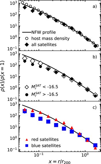
Figure 2. Normalized radial density profiles for the IllustrisTNG100 host−satellite systems. Black lines: NFW profile that best fits the mean radial mass density of the host galaxies (concentration parameter: c = 8.9). (a) Circles: mean radial mass density of the host galaxies; diamonds: mean radial number density of all satellite galaxies. (b) Diamonds: mean radial number density for satellites with Mr < −16.5; circles: mean radial number density for satellites with Mr > −16.5. (c) Mean satellite radial number density, computed separately for red and blue satellites.
Download figure:
Standard image High-resolution imageThe deviation between the shapes of the mean halo mass density profile and the satellite number density profile is explored further in Figures 2(b) and (c), where we subdivide the satellite sample by r-band absolute magnitude and (g − r) color. In Figure 2(b), we divide the satellites into the brightest 50% of the sample and the faintest 50% of the sample using the median satellite r-band absolute magnitude,  . From Figure 2(b), neither the brightest nor fainest satellites reproduce the shape of the mean halo mass density profile on scales ≲25% of the virial radius; however, the discrepancy between the mean halo mass density profile and the satellite number density profile is greater for the faintest satellites than it is for the brightest satellites. The spatial distributions of both the brightest and the faintest satellite galaxies are well fitted by NFW profiles with concentrations c = 4.2 and 2.3, respectively. That is, while both populations are distributed in a manner that is consistent with an NFW profile, both populations are less concentrated than the mean host mass density, and the spatial distribution of the faintest satellites is considerably less concentrated than the spatial distribution of the brightest satellites.
Figure 2(c) shows the dependence of the normalized radial number density profile on the satellites’ optical color (2366 red satellites vs. 1320 blue satellites). From Figure 2(c), neither red nor blue satellites reproduce the shape of the mean halo mass density profile over all scales at which satellites are found. In the case of the red satellites, the number density profile falls below that of the mean halo mass density profile on scales ≲10% of the virial radius. In the case of the blue satellites, the number density profile falls below that of the mean halo mass density profile on scales ≲50% of the virial radius. Additionally, the spatial distribution of the blue satellites is well fitted by an NFW profile with concentration c = 1.9; however, the spatial distribution of the red satellites is not well fitted by an NFW profile.
Next, we divide the full satellite sample into three parts according to their (g − r) colors. Figure 3 shows the individual contributions of the reddest one-third and bluest one-third of the complete satellite sample to the normalized number density profile that was computed using all TNG100 satellites (i.e., the results shown in Figure 2(a)). That is, in Figure 3 we do not normalize the number density profiles of the reddest and bluest satellites to unity at x = 1. Instead, they are normalized to the number density of all TNG100 satellites at x = 1. This allows us to determine what fraction of the number density profile for all satellites is associated with the reddest satellites versus the bluest satellites.
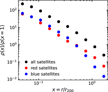
Figure 3. Contribution of the reddest one-third of all satellite galaxies and the bluest one-third of all satellite galaxies to the normalized radial number density profile that was obtained using the complete sample of TNG100 satellite galaxies.
Download figure:
Standard image High-resolution imageColored points in Figure 3 show results for the reddest one-third of all satellites ((g − r) > 0.69; red points) and the bluest one-third of all satellites ((g − r) < 0.59; blue points). From this, it is clear that the distributions of the reddest and bluest satellites contribute similar amounts to the overall satellite number density profile at small host−satellite separations. This is in stark contrast to the results of Sales et al. (2007), who applied the same host−satellite selection criteria to a semianalytic galaxy catalog that was constructed using the Millennium simulation. Sales et al. (2007) found that the distribution of the reddest one-third of their satellites was considerably more concentrated than was the distribution of the bluest one-third of their satellites. In the case of the Sales et al. (2007) satellites, 50% of the reddest one-third of the satellites were found within a host−satellite separation of 0.32r200, while 50% of the bluest one-third of the satellites were found within a host−satellite separation of 0.71r200. For the TNG100 satellites we find that 50% of the reddest one-third of the satellites are within 0.49r200 and 50% of the bluest one-third of the satellites are within 0.53r200. Compared to the results of Sales et al. (2007), the bluest and reddest TNG100 satellites are more equally distributed across the radial extent of the host. The difference in these simulated samples likely arises from the semianalytic model used by Sales et al. (2007), which assumed that satellites immediately lose their reservoir of star-forming gas when they are accreted by a host. This leads to a fast color transition from blue to red, resulting in blue satellites being found primarily in the outer regions of their hosts’ halos. In TNG100, gas must be removed from the satellites via hydrodynamical processes on a longer timescale, resulting in blue satellites that can exist for longer times within their hosts’ halos and, therefore, can be found at small host−satellite distances.
3.1. Comparison of TNG100 and Illustris-1 Host−Satellite Systems
As noted above, the models used for AGN feedback, galactic winds, and the growth of supermassive black holes in the IllustrisTNG100 simulation differed from those used in the Illustris-1 simulation. These modifications resulted in a significant change to the color distribution of present-day galaxies. In addition, they have the potential to affect both the mean host halo concentration and the spatial distribution of the satellites. Therefore, in Figure 4 we compare results from our TNG100 sample to results from an identically selected Illustris-1 sample (e.g., Brainerd 2018). In both the Illustris-1 sample and the TNG100 sample, the mean host mass density profiles are well fitted by NFW profiles, and the best-fitting NFW profiles for both sets of host galaxies are shown in Figure 4(a). From Brainerd (2018), the best-fitting NFW profile for the mass density of the Illustris-1 hosts has a concentration parameter of c = 11.9, which is considerably larger than the value of c = 8.9 that we find for the TNG100 hosts. This is consistent with the fact that the concentration parameters of galaxies in the original Illustris suite of simulations were higher than expected (see Pillepich et al. 2018a) and the updated models in the TNG suite of simulations resulted in galaxies that are less concentrated and better match observed galaxies.
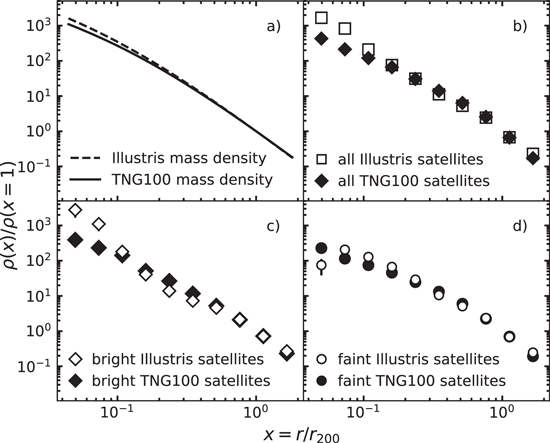
Figure 4. Comparison of TNG100 host−satellite systems and Illustris-1 host−satellite systems. (a) Best-fitting NFW profiles for the mean host mass densities. (b) Radial number density profiles obtained using all satellites. (c) Radial number density profiles obtained using only satellites with Mr < −16.5. (d) Radial number density profiles obtained using only satellites with Mr > −16.5.
Download figure:
Standard image High-resolution imageIn addition to differences in the mean host mass density, the satellite distributions in the two simulations also show differences. Figure 4(b) shows satellite radial number density profiles computed using all of the satellites in each simulation. From this, it is clear that the number density profile of the Illustris-1 satellites exceeds that of the TNG100 satellites on scales ≲10% of the virial radius, and the discrepancy is most pronounced for satellites brighter than Mr = −16.5 (see Figure 4(c)). For these bright satellites, the number density profiles from Illustris-1 and TNG100 show good agreement only on scales ≳0.6r200. On scales ≲0.1r200, the disagreement between the number density profiles for satellites with Mr < −16.5 correlates with the steep increase in the number density profile found by Brainerd (2018) for bright Illustris-1 satellites with small host−satellite separations. Since the two host−satellite samples were selected in exactly the same manner, one of the outcomes of the improved models in the TNG suite of simulations is the elimination of the steep increase in the satellite number density found by Brainerd (2018) at small host−satellite separations.
3.2. Dependence of Density Profiles on Host Luminosity and Color
In Figures 5–8 we subdivide the TNG100 host−satellite sample in various ways in order to explore the degree to which satellites in the subsamples trace the mean mass density profiles of their hosts. In all of these figures we compare the normalized satellite number density profile to the mean mass density of the corresponding host galaxies and list values of the reduced χ2 (i.e., the χ2 per degree of freedom, χ2/ν) for the comparisons in the individual panels.
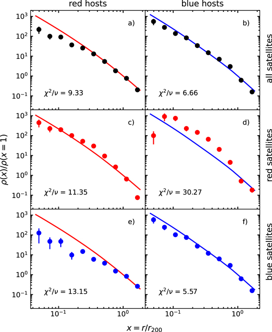
Figure 5. Normalized satellite number density profiles for color-based subdivisions of the host−satellite sample. (a) All satellites of red hosts. (b) All satellites of blue hosts. (c) Red satellites of red hosts. (d) Red satellites of blue hosts. (e) Blue satellites of red hosts. (f) Blue satellites of blue hosts. Solid lines in each panel show the mean mass density of the corresponding host galaxies (red line: red hosts; blue line: blue hosts). Each panel indicates the χ2 per degree of freedom for a comparison of the satellite number density profile to the mean host mass density profile.
Download figure:
Standard image High-resolution image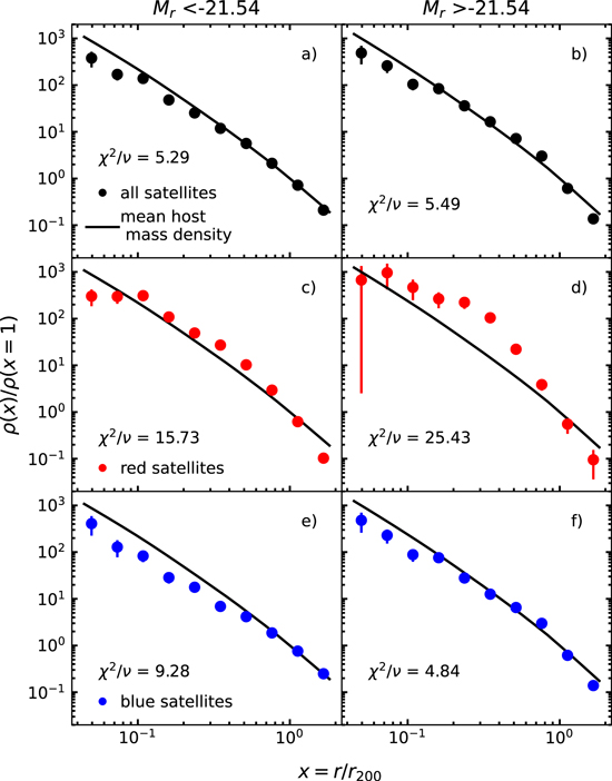
Figure 6. Normalized satellite number density profiles for luminosity-based subdivisions of the hosts and color-based subdivisions of the satellites. (a) All satellites of the brightest 50% of host galaxies. (b) All satellites of the faintest 50% of host galaxies. (c) Red satellites of the brightest 50% of host galaxies. (d) Red satellites of the faintest 50% of host galaxies. (e) Blue satellites of the brightest 50% of host galaxies. (f) Blue satellites of the faintest 50% of host galaxies. Solid black lines in each panel show the mean mass density of the corresponding host galaxies. Each panel indicates the χ2 per degree of freedom for a comparison of the satellite number density profile to the mean host mass density profile.
Download figure:
Standard image High-resolution image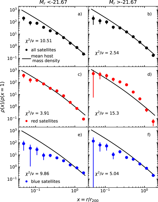
Figure 7. Same as Figure 6, but with the sample restricted to red host galaxies and their satellites.
Download figure:
Standard image High-resolution image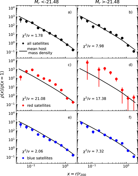
Figure 8. Same as Figure 6, but with the sample restricted to blue host galaxies and their satellites.
Download figure:
Standard image High-resolution imageFigure 5 shows results for the host−satellite sample subdivided by host and satellite color. The left panels of Figure 5 show results for the satellites of red host galaxies, while the right panels show results for the satellites of blue host galaxies. The top panels of Figure 5 show the results for all satellites that surround each type of host galaxy, the middle panels show the results for the red satellites that surround each type of host galaxy, and the bottom panels show the results for the blue satellites that surround each type of host galaxy. Formally, none of the host mass density profiles are a good fit to any of the satellite number density profiles (i.e., χ2/ν ≫ 1 in all cases). Given that, on average, the red satellites are an older population than are the blue satellites, it might be expected that the red satellites would be good tracers of the hosts’ mass distributions, particularly in the case of red host galaxies. From Figure 5, the red satellites are better tracers of the mean mass density that surrounds the red hosts than are the blue satellites. However, the detailed shape of the number density profile for the red satellites of red hosts cannot be fitted by an NFW profile, and the value of the reduced χ2 (11.35) indicates that red satellites do not trace the mass density of the red hosts well. The best agreement between a satellite number density profile and a host mass density profile in Figure 5 occurs for the blue satellites of blue hosts (i.e., Figure 5(f)). While the agreement is not formally good for blue satellites of blue hosts (χ2/ν = 5.57), it is better than the agreement for either the red satellites of blue hosts or all satellites of blue hosts. Importantly, the level of disagreement between the host mass distributions and the satellite distributions is such that none of the satellite distributions in Figure 5 could be used to recover accurate host mass density profiles.
In Figures 6–8 we explore the degree to which the satellite distribution traces the mass distribution surrounding hosts of differing luminosity. In each of these figures, we use the median host magnitude to divide the host sample in half. In Figure 6, all host galaxies are included in the analyses. In Figures 7 and 8 we further subdivide the hosts by their colors. As in Figure 5, in Figures 6–8 we also subdivide the satellites according to their colors. Also as in Figure 5, none of the host mass density profiles are a good fit to any of the satellite number density profiles over all host−satellite separations for which satellites are identified. In addition, the sense of the disagreement between the host mass density profiles and the number density profiles for the red satellites is often opposite to the sense of the disagreement between the host mass density and the number density profiles for the blue satellites. These systematic, but opposite, differences can combine to give a better agreement between the host mass density profile and the number density profile that is obtained when all satellite galaxies are included in the calculation than when calculated for either red or blue satellites alone. This effect can be seen in the left columns of Figures 6 and 8 and the right column of Figure 7.
Among all the results shown in Figures 6–8, by far the best agreement between the shape of the satellite number density profile and the shape of the host mass density profile occurs for the complete sample of satellite galaxies that surround the brightest blue host galaxies (i.e., Figure 8(a), for which χ2/ν = 1.78). This moderate agreement between the spatial distribution of the complete sample of satellites and the mean mass density surrounding the brightest blue host galaxies is, nevertheless, somewhat coincidental. That is, the number density profile of the blue satellites (which are the majority of the satellites in this case) falls systematically below the mean mass density of the brightest blue host galaxies on scales ≲0.4r200. However, the number density profile of the red satellites rises systematically above the mean mass density of the brightest blue host galaxies on scales 0.07r200 ≲r ≲ 0.7r200. It is only through the combination of these opposite, systematic differences that the shape of the number density profile of the complete sample of satellite galaxies agrees moderately well with the shape of the mass density profile of the brightest blue host galaxies.
3.3. Dependence of Satellite Number Density Profiles on Joining Redshift
On average, the red TNG100 satellites joined their hosts at earlier times than did the blue satellites (see Section 2). Because of this, present-day satellite color is a proxy for the relative ages of the satellites, and it might be expected that red satellites will therefore be the best tracers of the host mass distribution. However, this expectation presupposes that the earliest satellites to join their hosts will, in fact, be good tracers of the host’s mass, and we have seen above that red TNG100 satellites are not, in general, good tracers of their host’s mass distributions.
In an observational sample, the joining times of the satellite galaxies are, of course, not known. Because of this, it is useful to have a proxy such as color to distinguish “old” satellites from “young” satellites in an observational sample. In a simulated sample, however, it is straightforward to determine the redshifts at which the satellites joined their hosts, and so it is not absolutely necessary to rely on proxies to separate “young” from “old” satellites in a simulated sample.
In this section, we compare the normalized number density profiles for subsets of satellites that joined their hosts in the distant past to those for satellites that joined their hosts only recently. To do this, we divide the full satellite sample into thirds using the joining redshift, zj
. Figure 9 shows the normalized number density profiles for the oldest one-third of the satellites (median joining redshift:  ) and the youngest one-third of the satellites (median joining redshift:
  ), along with the mean host mass density profiles.
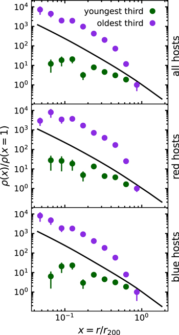
Figure 9. Normalized satellite number density profiles, computed separately for the oldest one-third of the satellites (purple points) and the youngest one-third of the satellites (green points). “Ages” of the satellites are determined by the redshift at which they first entered the virial radius of their host (see text). Top: all host−satellite systems. Middle: host−satellite systems with red hosts. Bottom: host−satellite systems with blue hosts. In each panel black lines show the mean mass densities for the corresponding host galaxies.
Download figure:
Standard image High-resolution imageFrom Figure 9, neither the oldest nor the youngest satellites have normalized number density profiles that match the shape of the mean host mass density profiles. Number density profiles for the youngest satellites fall systematically below the host mass density profiles, and number density profiles for the oldest satellites rise systematically above the host mass density profiles. This is true within the full sample (top panel) and samples that are subdivided by host color (middle and bottom panels).
It is unsurprising that the youngest satellites do not trace the mass density of their hosts since the expectation is that they have not had time to come into virial equilibrium with the hosts. That is, the dynamical time for a spherical halo is  (see, e.g., Gan et al. 2010), so the amount of cosmic time that passes between zj
= 0.074 (i.e., the median joining redshift of the youngest satellites) and the present is ∼1 Gyr, or ∼0.7τdyn. In the case of the oldest satellites, the amount of cosmic time that passes between the median joining redshift (zj
= 0.79) and the present day is ∼5τdyn and, based on the dynamical time alone, one might expect the oldest satellites to be in approximate equilibrium with their hosts’ dark matter halos. However, infalling satellites ought to be subject to dynamical friction, which will drive them toward the centers of their hosts’ dark matter halos.
(see, e.g., Gan et al. 2010), so the amount of cosmic time that passes between zj
= 0.074 (i.e., the median joining redshift of the youngest satellites) and the present is ∼1 Gyr, or ∼0.7τdyn. In the case of the oldest satellites, the amount of cosmic time that passes between the median joining redshift (zj
= 0.79) and the present day is ∼5τdyn and, based on the dynamical time alone, one might expect the oldest satellites to be in approximate equilibrium with their hosts’ dark matter halos. However, infalling satellites ought to be subject to dynamical friction, which will drive them toward the centers of their hosts’ dark matter halos.
Gan et al. (2010) showed that the dynamical friction time for satellites is highly sensitive to the efficiency with which the satellites are tidally stripped. However, Gan et al. (2010) also found that the dynamical friction time for satellites with masses <25% of the mass of their host should range from ≲2 Gyr for satellites on relatively circular orbits to ∼5 Gyr for satellites on radial orbits, independent of the degree of tidal stripping. Since the TNG100 satellites are typically orders of magnitude less massive than their hosts, and since the amount of cosmic time that passes between zj = 0.79 and the present day is ∼7 Gyr, it is likely that dynamical friction will have affected the present-day locations of the oldest satellites. Therefore, compared to the mean host mass density, the oldest satellites should be more concentrated toward the centers of the host−satellite systems (as, indeed, is the case in Figure 9).
4. Summary and Discussion
The NFW density profile is motivated by CDM simulations that show that the complex interactions of particles over time cause the mass to settle into this distinct shape, regardless of the cosmology. An important question, then, is whether the spatial distribution of satellite galaxies should be expected to follow a similar profile and, hence, whether the spatial distribution of satellite galaxies in the observed universe can be used to directly constrain the concentration of the mass that surrounds the satellites’ host galaxies.
Here we have compared normalized radial number density profiles for the satellites of isolated host galaxies in the IllustrisTNG100 simulation to the mean mass densities of the host galaxies. The host−satellite systems were selected using the same criteria that were adopted by Brainerd (2018) for the Illustris-1 simulation and by Sales et al. (2007) for a galaxy catalog obtained by applying a SAM to the Millennium simulation.
In agreement with Sales et al. (2007), we find that the number density profile of the complete sample of TNG100 satellites is well fitted by an NFW profile. In contrast to the results of Sales et al. (2007), who concluded that their satellites were only slightly less concentrated than the host mass distribution, the concentration of the TNG100 satellites is a factor of ∼2 lower than that of the mean host mass density. In agreement with Brainerd (2018), we find that the number density profile of the complete sample of TNG100 satellites does not follow the shape of the mean host mass density profile; however, despite being selected in the same way from simulations with identical initial conditions, there are distinct differences between the satellite number density profiles for the TNG100 and Illustris-1 satellites. In particular, the distribution of the TNG100 satellites does not show the steep increase in number density at small host−satellite separations that was found by Brainerd (2018). Since the key difference between the IllustrisTNG100 simulation and the original Illustris-1 simulation is the manner in which galactic winds, AGN feedback, and the growth of supermassive black holes were treated, it is likely that the shape of the satellite distribution at small host−satellite separations is particularly sensitive to these aspects of the galaxy formation model.
In subdividing the host−satellite sample according to host and satellite color, as well as host and satellite luminosity, we find that no population of TNG100 satellites yields a number density profile that is formally in good agreement with the shape of the mean host mass density profile (i.e., χ2/ν exceeds unity in all cases). While there are examples of moderately good agreement when all satellites that surround the host galaxies are considered, the agreement is somewhat coincidental. This is due to the number density profiles of red satellites and blue satellites being systematically offset in opposite directions from the mean host mass density profile (i.e., the number density profile for blue satellites falls below that of the mass density, while the number density profile for red satellites rises above that of the mass density).
Unlike Sales et al. (2007), who found that the distribution of the reddest satellites was considerably more concentrated than the distribution of the bluest satellites, we find that, for host−satellite separations ≲0.5r200, the distribution of the reddest TNG100 satellites is similar to that of the bluest TNG100 satellites. The difference between these two results may be attributable to the SAM used by Sales et al. (2007) causing the satellites to quickly lose their gas reservoirs upon accretion by their hosts. This would have stifled future star formation in the accreted satellites, resulting in blue satellites turning red over relatively short timescales.
Lastly, if infalling satellites are expected to come into equilibrium with their hosts’ dark matter halos, this should take place over an extended period of time, and satellites that joined their hosts in the distant past might be expected to be the best tracers of the mean host mass density. However, when we investigate the locations of the satellites as a function of the redshift at which they joined their hosts, we find that neither the youngest nor the oldest satellites trace the mean host mass density. This indicates that while time since joining a system is a major factor in determining the shape of the satellite number density profile, it is not a reliable predictor of the satellite population that best traces the host mass distribution. In the case of the youngest one-third of the satellites, not enough time has passed for their spatial distribution to become as concentrated as the mean mass density of their hosts. In the case of the oldest one-third of the satellites, the majority of the satellites joined their host sufficiently far in the past that dynamical friction has likely driven them toward the centers of the systems, resulting in satellite distributions that are more concentrated than the mean host mass density.
5. Conclusions
Our work shows that the shapes of the TNG100 satellite number density profiles, as well as the degree to which they agree with their hosts’ mass density profiles, are sensitive to the properties of the hosts and satellites that are used in the analysis (i.e., luminosity, color, satellite joining time). Even samples consisting only of satellites that have had time to virialize within their hosts’ halos fail to trace their hosts’ mass density. While the oldest satellites are more concentrated than the mean host mass density, the youngest satellites are less concentrated than the mean host mass density. One possible explanation for this phenomenon is that once satellites enter their hosts’ halos, dynamical friction drives them toward the centers of the halos. However, host−satellite samples that are drawn from different simulations, but using identical selection criteria, also show distinct differences between their satellite number density profiles (Sales et al. 2007; Brainerd 2018; this work). This suggests that the satellite number density profiles can also be sensitive to the galaxy formation models adopted by the simulations. The root causes of all of these differences cannot be identified categorically from the work presented here, and we will explore them in more detail in a future analysis. The major conclusion from our analysis is that, if we live in a ΛCDM universe, it is not clear that the observed satellites of isolated host galaxies will be reliable tracers of their hosts’ dark matter halos. Therefore, it is not clear that halo properties of isolated galaxies that are inferred from observed satellite distributions are, in fact, accurate representations of the underlying halo properties.
We are grateful to the anonymous reviewer for helpful suggestions that improved the paper. This work was partially supported by National Science Foundation grant AST-2009397 and a Summer 2021 Massachusetts Space Grant Fellowship.