Abstract
The roles that mass and environment play in galaxy quenching are still under debate. Leveraging the Photometric objects Around Cosmic webs method, we analyze the excess surface distribution  of photometric galaxies in different colors (rest-frame u − r) within the stellar mass range of 109.0 ∼ 1011.0M⊙ around spectroscopic massive central galaxies (1010.9 ∼ 1011.7M⊙) at the redshift interval of 0 < zs < 0.7, utilizing data from the Hyper Suprime-Cam Subaru Strategic Program and the spectroscopic samples of Slogan Digital Sky Survey (i.e., Main, LOWZ, and CMASS samples). We find that both mass and environmental quenching contribute to the evolution of companion galaxies. To isolate the environmental effect, we quantify the quenched fraction excess (QFE) of companion galaxies encircling massive central galaxies within 0.01h−1 Mpc < rp < 20h−1 Mpc, representing the surplus quenched fraction relative to the average. We find that the high-density halo environment affects star formation quenching up to about three times the virial radius, and this effect becomes stronger at lower redshift. We also find that even after being scaled by the virial radius, the environmental quenching efficiency is higher for more massive halos or for companion galaxies of higher stellar mass, though the trends are quite weak. We present a fitting formula that comprehensively captures the QFE across central and companion stellar mass bins, halo-centric distance bins, and redshift bins, offering a valuable tool for constraining galaxy formation models. Furthermore, we have made a quantitative comparison with IllustrisTNG that underscores some important differences, particularly in the excessive quenching of low-mass companion galaxies (<109.5M⊙) in the simulation.
Original content from this work may be used under the terms of the Creative Commons Attribution 4.0 licence. Any further distribution of this work must maintain attribution to the author(s) and the title of the work, journal citation and DOI.
1. Introduction
Nowadays, it is generally adopted that galaxies can be divided into two main populations: star-forming and passive. The former kind of galaxies are typically young, forming new stars, and have blue colors along with late-type morphologies. The latter kind of galaxies are typically old, do not show star formation activity, and have red colors and early-type morphologies (Blanton et al. 2003; Baldry et al. 2004; Kauffmann et al. 2003, 2004; Cassata et al. 2008; Wetzel et al. 2012; van der Wel et al. 2014; Davies et al. 2019; Pallero et al. 2019). In order to understand these galaxy properties, a series of physical processes in galaxy formation and evolution should be taken into account. Among them, galaxy quenching plays a remarkable role in shaping galaxy properties such as color and morphology (Blanton et al. 2003; Baldry et al. 2004; Brinchmann et al. 2004; Cassata et al. 2008; Muzzin et al. 2013; Davies et al. 2019; Pallero et al. 2019). Thus, a deep investigation of galaxy quenching will ultimately be a major step forward in our understanding of galaxy formation and evolution.
Mass quenching and environmental quenching are the two dominant modes (Peng et al. 2010, 2012; Cooper et al. 2010; Sobral et al. 2011; Muzzin et al. 2013; Darvish et al. 2016; Zu & Mandelbaum 2016; Schaefer et al. 2017, 2019; Contini et al. 2020; Chartab et al. 2020; Einasto et al. 2022; Taamoli et al. 2024). Mass quenching refers to all the internal processes that quench star formation and are expected to be primarily dependent on the galaxy mass. Relying on the characteristic stellar mass regimes, distinct processes have been proposed. In the low stellar mass regime (![$\mathrm{log}[{M}_{\star }/{M}_{\odot }]\lt 10$](https://content.cld.iop.org/journals/0004-637X/969/2/129/revision1/apjad47f7ieqn2.gif) ), gas outflows, which are attributed to stellar feedback processes, such as stellar winds or supernova explosions, have a significant impact on inhibiting star formation (Larson 1974; Dekel & Silk 1986; Dalla Vecchia & Schaye 2008). In the high stellar mass regime (
), gas outflows, which are attributed to stellar feedback processes, such as stellar winds or supernova explosions, have a significant impact on inhibiting star formation (Larson 1974; Dekel & Silk 1986; Dalla Vecchia & Schaye 2008). In the high stellar mass regime (![$\mathrm{log}[{M}_{\star }/{M}_{\odot }]\gt 10$](https://content.cld.iop.org/journals/0004-637X/969/2/129/revision1/apjad47f7ieqn3.gif) ), active galactic nucleusfeedback is expected to be more effective in quenching star formation (Croton et al. 2006; Nandra et al. 2007; Fabian 2012; Fang et al. 2013; Cicone et al. 2014; Bremer et al. 2018). Environmental quenching is driven by the interactions between galaxies and their local environment, such as ram pressure stripping (Gunn & Gott 1972; Moore et al. 1999; Brown et al. 2017; Poggianti et al. 2017; Barsanti et al. 2018; Owers et al. 2019; Cortese et al. 2021), strangulation or starvation (Larson et al. 1980; Moore et al. 1999; Nichols & Bland-Hawthorn 2011; Peng et al. 2015), and harassment (Farouki & Shapiro 1981; Moore et al. 1996). Ram pressure stripping occurs when a galaxy moves through the intracluster medium. If the ram pressure is strong enough, it may strip a galaxy of its entire cold gas reservoir and give rise to an abrupt quenching of its star formation. Strangulation, which assumes that a galaxy's gas reservoir is cut off when it is accreted into a larger host system, results in a decline of the galaxy's star formation rate as it runs out of fuel. Harassment refers to the cumulative effect of multiple high-speed impulsive encounters, which can result in the removal of gas.
), active galactic nucleusfeedback is expected to be more effective in quenching star formation (Croton et al. 2006; Nandra et al. 2007; Fabian 2012; Fang et al. 2013; Cicone et al. 2014; Bremer et al. 2018). Environmental quenching is driven by the interactions between galaxies and their local environment, such as ram pressure stripping (Gunn & Gott 1972; Moore et al. 1999; Brown et al. 2017; Poggianti et al. 2017; Barsanti et al. 2018; Owers et al. 2019; Cortese et al. 2021), strangulation or starvation (Larson et al. 1980; Moore et al. 1999; Nichols & Bland-Hawthorn 2011; Peng et al. 2015), and harassment (Farouki & Shapiro 1981; Moore et al. 1996). Ram pressure stripping occurs when a galaxy moves through the intracluster medium. If the ram pressure is strong enough, it may strip a galaxy of its entire cold gas reservoir and give rise to an abrupt quenching of its star formation. Strangulation, which assumes that a galaxy's gas reservoir is cut off when it is accreted into a larger host system, results in a decline of the galaxy's star formation rate as it runs out of fuel. Harassment refers to the cumulative effect of multiple high-speed impulsive encounters, which can result in the removal of gas.
In the past few years, many studies have focused on which mode dominates the quenching of galaxies. It is generally thought that central galaxies, which are the most massive galaxies residing at the centers of dark matter halos, strongly depend on mass quenching (e.g., Peng et al. 2010). However, the quenching mechanism for satellite galaxies remains a subject of ongoing debate. Many observational results have shown that satellite galaxies are more likely to be quenched in a denser environment (Balogh et al. 2000; Blanton & Berlind 2007; Tal et al. 2014; Schaefer et al. 2017). While others have shown no or little dependence on the proxies for the environment, such as halo mass and cluster-centric distance (Muzzin et al. 2012; Darvish et al. 2016; Laganá & Ulmer 2018). To elucidate the diverse influences on galaxy quenching, comparisons between observational results and simulations are invaluable. For example, Contini et al. (2020) explored the roles of environment and stellar mass in quenching galaxies using the merger tree of an N-body simulation presented in Kang et al. (2012). Additionally, Engler et al. (2023) quantitatively examined quenched fractions, gas content, and stellar mass assembly of satellite galaxies around MW/M31-like hosts in TNG50, the highest-resolution run of the IllustrisTNG simulations (Nelson et al. 2019). In another study, Pan et al. (2023) compared simulated satellite galaxies from the Auriga simulations (Grand et al. 2017) with observed satellite galaxies from the ELVES Survey (Carlsten et al. 2022), revealing consistent properties, such as quenched fraction and the luminosity function. Despite notable advancements in hydrodynamic simulations, satellite properties still hinge on sub-grid physical recipes. An accurate delineation of mass and environmental quenching mechanisms holds the potential to provide crucial insights for refining sub-grid physics in galaxy formation models. To refine galaxy quenching models, it is essential to gather observed galaxy color distributions across broad stellar mass ranges and diverse environments. In this study, we employ the Photometric objects Around Cosmic webs (PAC) method, developed in the inaugural paper of this series (Xu et al. 2022b, hereafter Paper I) built on the work by Wang et al. (2011). Leveraging large and deep photometric surveys, we quantify the excess surface density distribution of both blue and red companion galaxies encircling massive central galaxies. Our analysis extends to the very faint end (109.0 M⊙) and encompasses redshifts up to zs ≈ 0.7. 6 By amalgamating the aforementioned outcomes, we delve into the study of the quenched fraction excess (QFE) of companion galaxies attributed to environmental effects. Our findings reveal that environmental quenching predominantly occurs in high-density regions within massive dark matter halos, up to three times the virial radius (3rvir). Using the QFE, we quantify the efficiency of quenching in different environments. A fitting model for the QFE is constructed, accounting for dependencies on halo-centric distance, halo mass, companion stellar mass, and redshift. Additionally, we compare our results with those from the TNG300 cosmological hydrodynamical simulation, revealing an over-quenching of low-mass galaxies by environmental factors in TNG.
We adopt the Planck 2018 ΛCDM cosmological model (Planck Collaboration et al. 2020) with Ωm,0 = 0.3111, ΩΛ,0 = 0.6889, and H0 = 67.66 km s−1 Mpc−1 throughout the paper.
2. Data and Method
2.1. PAC
We introduced a method to estimate the projected density distribution  of photometric objects with specific physical properties (e.g., luminosity, mass, color) around spectroscopic objects in Paper I:
Here, wp(rp) and ω12,weight(ϑ) represent the projected cross-correlation function (PCCF) and the weighted angular cross-correlation function (ACCF) between a specified set of spectroscopically identified galaxies and a sample of photometric galaxies. Additionally,  and
and  denote the mean number density and mean angular surface density of the photometric galaxies, while r1 signifies the comoving distance to the spectroscopic galaxies. The weight in ω12,weight(ϑ) is incorporated to account for the variation in rp at a given angle θ due to galaxies being at different redshifts, where rp = r1
θ. We employ the Landy–Szalay estimator for the two-point correlation function (Landy & Szalay 1993). A notable strength of PAC lies in its ability to statistically estimate the rest-frame physical properties of photometric objects. The key steps of PAC are as follows:
denote the mean number density and mean angular surface density of the photometric galaxies, while r1 signifies the comoving distance to the spectroscopic galaxies. The weight in ω12,weight(ϑ) is incorporated to account for the variation in rp at a given angle θ due to galaxies being at different redshifts, where rp = r1
θ. We employ the Landy–Szalay estimator for the two-point correlation function (Landy & Szalay 1993). A notable strength of PAC lies in its ability to statistically estimate the rest-frame physical properties of photometric objects. The key steps of PAC are as follows:
- (1)Split the spectroscopic catalogs into narrower redshift bins to limit the range of r1 in each bin.
- (2)Assume that all photometric objects share the same redshift as the mean redshift in each redshift bin and compute the physical properties of the photometric objects. Consequently, there exists a physical property catalog for the photometric sample in each redshift bin.
- (3)Select photometric objects with specific physical properties from the catalog and calculate
 using Equation (1) in each redshift bin. Because foreground and background sources along the line of sight (LOS) to a spectroscopic galaxy are distributed statistically in the same way as those along a random LOS, the foreground and background objects with the wrong properties can be canceled out through ACCF, and only photometric objects around the spectroscopic galaxy with the correct redshift and physical properties can contribute to the ACCF.
 - (4)Aggregate the results from different redshift bins and average them with appropriate weights.

For a more comprehensive understanding, we refer the reader to Wang et al. (2011) and Paper I. To validate this method, we compare the  results obtained by PAC with those directly obtained from the spectroscopic sample. The comparison confirms the reliability of PAC. The details are provided in Appendix A.
2.2. Observational Data
In this subsection, we outline the data from spectroscopic and photometric catalogs utilized in this paper across three distinct redshift ranges.
2.2.1. Selection of Central Galaxies
Focusing on central galaxies within the spectroscopic sample, we define centrals as galaxies that do not have more massive neighbors within a distance of  along the LOS and within
  perpendicular to the LOS. Here,
  denotes the virial radius of the more massive galaxies in comparison. We adopt this relatively conservative criterion for central galaxy selection, recognizing that the environmental impact of a halo extends up to approximately 3rvir as we will show below. As shown by Oliva-Altamirano et al. (2014), about 13% of the central galaxies thus defined may not be at the centers of the host halo gravitational wells. Since most of these off-centering galaxies are still with the gravitational well and the fraction is small, we believe this population should not have a significant impact on our results below.
In this analysis, we determine the values of rvir by replicating the methodology outlined in Xu et al. (2023, hereafter Paper IV), leveraging the high-resolution Jiutian
N-body simulation (J. Han et al. 2024, in preparation). Our objective is to constrain the stellar–halo mass relations (SHMR) under the Planck 2018 cosmology through the application of the subhalo abundance matching method. The Jiutian simulation features 61443 dark matter particles within a periodic box of 1000h−1 Mpc, providing a sufficiently large volume for robustly modeling  up to scales of 20h−1 Mpc. Dark matter halos are identified using the Friends-of-Friends method, and subhalos are traced using HBT+ (Han et al. 2012, 2018). We adopt the double power-law form (DP model in Paper IV) for the SHMR:
Here, M* is the stellar mass, Macc is defined as the viral mass Mvir of the halo at the time when the galaxy was last the central dominant object. The scatter in  at a given Macc is described with a Gaussian function of the width σ. α and β represent the slopes of the SHMR at high- and low-mass ends, respectively. The constrained parameters for the DP model across three redshift ranges are detailed in Table 1. For the purposes of this paper, we employ interpolation to obtain parameter values for the intermediate redshift bin 0.3 < zs
< 0.5. The SHMR for different redshift bins in this work are shown in Figure 1. To derive the halo virial mass Mvir, we use the stellar mass of the central galaxy based on the SHMR. Subsequently, we calculate the corresponding rvir by computing mean values within each stellar mass bin. The values of rvir and the standard deviation for various central stellar mass bins utilized in this study are presented in Table 2. The values of Mvir and the scatter for various central stellar mass bins are presented in Table 3. In this work, we use the mean values to construct our model.
at a given Macc is described with a Gaussian function of the width σ. α and β represent the slopes of the SHMR at high- and low-mass ends, respectively. The constrained parameters for the DP model across three redshift ranges are detailed in Table 1. For the purposes of this paper, we employ interpolation to obtain parameter values for the intermediate redshift bin 0.3 < zs
< 0.5. The SHMR for different redshift bins in this work are shown in Figure 1. To derive the halo virial mass Mvir, we use the stellar mass of the central galaxy based on the SHMR. Subsequently, we calculate the corresponding rvir by computing mean values within each stellar mass bin. The values of rvir and the standard deviation for various central stellar mass bins utilized in this study are presented in Table 2. The values of Mvir and the scatter for various central stellar mass bins are presented in Table 3. In this work, we use the mean values to construct our model.
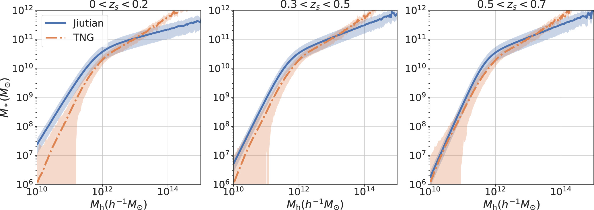
Figure 1. The central SHMR of Jiutian and TNG for three distinct redshift bins: 0 < zs < 0.2 (left), 0.3 < zs < 0.5 (medium), and 0.5 < zs < 0.7 (right). Solid blue lines denote Jiutian simulation, while dotted red lines are for TNG.
Download figure:
Standard image High-resolution imageTable 1. The Marginalized Posterior PDFs of the Parameters
| Redshift | Model |

| α | β |

| σ |
|---|---|---|---|---|---|---|
| zs < 0.2 | DP |

|

|

|

|

|
| 0.2 < zs < 0.4 | DP |

|

|

|

|

|
| 0.5 < zs < 0.7 | DP |

|

|

|

|

|
Note. M0 is in units of h−1 M⊙ and k is in units of M⊙.
Download table as: ASCIITypeset image
Table 2. rvir Derived from Jiutian and TNG for Different Central Stellar Mass Bins at Three Different Redshift Bins, with rvir in Units of h−1 Mpc
| Simulation | Redshift Bin | Mass Bin 
| |||
|---|---|---|---|---|---|
| 10.9–11.1 | 11.1–11.3 | 11.3–11.5 | 11.5–11.7 | ||
| Jiutian | zs < 0.2 | 0.355 ± 0.131 | 0.455 ± 0.186 | 0.597 ± 0.254 | 0.782 ± 0.323 |
| 0.3 < zs < 0.5 | 0.655 ± 0.211 | 0.848 ± 0.261 | |||
| 0.5 < zs < 0.7 | 0.622 ± 0.207 | 0.795 ± 0.256 | |||
| TNG | zs < 0.2 | 0.417 ± 0.069 | 0.515 ± 0.082 | 0.644 ± 0.094 | 0.789 ± 0.104 |
| 0.3 < zs < 0.5 | 0.681 ± 0.096 | 0.846 ± 0.117 | |||
| 0.5 < zs < 0.7 | 0.694 ± 0.102 | 0.848 ± 0.117 | |||
Download table as: ASCIITypeset image
Table 3.
 Derived from Jiutian for Different Central Stellar Mass Bins at Three Different Redshift Bins, with Mvir in Units of h−1
M⊙
Derived from Jiutian for Different Central Stellar Mass Bins at Three Different Redshift Bins, with Mvir in Units of h−1
M⊙
| Simulation | Redshift Bin | Mass Bin 
| |||
|---|---|---|---|---|---|
| 10.9–11.1 | 11.1–11.3 | 11.3–11.5 | 11.5–11.7 | ||
| Jiutian | zs < 0.2 | 12.859 ± 0.265 | 13.217 ± 0.263 | 13.575 ± 0.290 | 13.917 ± 0.352 |
| 0.3 < zs < 0.5 | 13.519 ± 0.590 | 13.844 ± 0.791 | |||
| 0.5 < zs < 0.7 | 13.424 ± 0.523 | 13.739 ± 0.637 | |||
Download table as: ASCIITypeset image
2.2.2. Redshift Range: 0.0 ∼ 0.2
For the photometric sample, we use the datasweep catalog of the Sloan Digital Sky Survey (SDSS) DR13 (Albareti et al. 2017). It contains a subset of the data from the full SDSS photometric catalogs, which is sufficient for our study. We select all galaxies with r-band apparent model magnitudes of r < 21.0. We also check the bitmask called RESOLVE_STATUES to select unique objects in the catalog. Then we trim the catalog by the MANGLE software (Hamilton & Tegmark 2004; Swanson et al. 2008) according to the geometry with the bright star masks cut out provided by the New York University Value Added Galaxy Catalog (NYU-VAGC) 7 (Blanton et al. 2005). We also restrict the galaxies to the continuous area of the North Galactic Cap (NGC). Finally, we obtain a photometric catalog with five bands ugriz. We also construct a random catalog with the same selection criteria as the photometric sample using the MANGLE software.
We employ the spectral energy distribution (SED) code CIGALE (Boquien et al. 2019) to compute the physical properties (e.g., stellar mass and rest-frame colors) of galaxies. The stellar population synthesis models of Bruzual & Charlot (2003) and the initial mass function from Chabrier (2003) are selected. We assume a delayed star formation history  , where τ spans from 107–1.258 × 10¹⁰ yr with an equal logarithmic interval
  . The extinction law of Calzetti et al. (2000) is adopted, with dust reddening in the range of 0 < E(B − V) < 0.5. Moreover, we set three metallicities, Z/Z⊙ equal to 0.4, 1, and 2.5, respectively, where Z⊙ is the metallicity of the Sun.
The spectroscopic galaxy sample is derived from the SDSS Data Release 7 (DR7; Abazajian et al. 2009) Main sample, which is contained in the NYU-VAGC. Initially, we select galaxies within the continuous region of the NGC with redshifts ranging from 0.0 < zs < 0.2. The physical properties of these galaxies are determined through SED modeling with the five bands ugriz. By applying the previously mentioned central selection criterion, we obtain the spectroscopic catalog. A random catalog for this spectroscopic sample is also constructed using MANGLE. The final effective area is 7032 deg2.
2.2.3. Redshift Range: 0.3 ∼ 0.5
We utilize the Wide layer photometric catalog from the second public data release (PDR2) of the Hyper Suprime-Cam (HSC) Subaru Strategic Program (Aihara et al. 2019) to construct the photometric sample within this redshift range. We select sources within the footprints observed with all five bands (grizy) to ensure sufficient bands for accurate physical property estimation through SED modeling. The 5σ depth for grizy are 26.6, 26.2, 26.2, 25.3, and 24.5, respectively. We mask sources around bright objects using the {grizy}_mask_pdr2_bright_objectcenter flag provided by the HSC Collaboration (Coupon et al. 2018). Additionally, the {grizy}_extendedness_value flag is employed to exclude stars from the sample.
For the spectroscopic catalog, we utilize the LOWZ sample and the CMASS sample from the Baryon Oscillation Spectroscopic Survey (BOSS; Ahn et al. 2012; Bolton et al. 2012). 8 The LOWZ database has a smaller footprint than CMASS because the galaxies from the first 9 months of the BOSS observation are removed due to the incorrect star-galaxy separation criterion. In total, the LOWZ database covers 8337 deg2 of the sky, with 5836 deg2 in the NGC and 2501 deg2 in the Southern Galactic Cap (SGC). CMASS covers 9376 deg2 of the sky, with 6851 deg2 in the NGC and 2525 deg2 in the SGC. Initially, we select galaxies in the redshift range of 0.3 ∼ 0.5. Subsequently, we match this spectroscopic catalog with the HSC photometric sample to obtain magnitudes in the grizy bands for each LOWZ and CMASS galaxy, allowing us to calculate their physical properties. Next, we select central galaxies to obtain the final spectroscopic catalog.
Moreover, we construct a random catalog for the photometric sample using the same selection criteria from the HSC database. Regarding the spectroscopic catalog, we emphasize the need to generate separate random catalogs for the LOWZ sample and the CMASS sample due to their different footprints. We first generate a random catalog in the HSC footprint and then apply the LSS geometry mask 9 provided by BOSS. For the LOWZ catalog, we apply mask_DR12v5_LOWZ_South.ply and mask_DR12v5_LOWZ_North.ply to obtain the corresponding random sample. Similarly, for the CMASS catalog, we use mask_DR12v5_CMASS_South.ply and mask_DR12v5_CMASS_North.ply. From these two random samples, we calculate the final effective areas of the LOWZ and CMASS catalogs as 338 and 458 deg2, respectively. The final spectroscopic sample and its random sample are a combination of the LOWZ and CMASS corresponding samples.
2.2.4. Redshift Range: 0.5 ∼ 0.7
In this redshift range, we employ the same HSC photometric sample mentioned above as the photometric catalog.
For the spectroscopic sample in this redshift range, we select the CMASS sample as mentioned previously. Initially, we choose galaxies within the redshift range of 0.5 ∼ 0.7. Subsequently, we follow the same steps mentioned earlier to construct both the spectroscopic catalog and the random catalog.
2.3. Completeness and Designs
Building upon previous studies (Xu et al. 2022a, hereafter Paper III), we define the stellar mass range for central galaxies from spectroscopic samples as [1010.9, 1011.7]M⊙ for zs < 0.2 and [1011.3, 1011.7]M⊙ for both 0.3 < zs < 0.5 and 0.5 < zs < 0.7. In the three redshift bins, there are 73,446, 4472, and 10,039 massive central galaxies, respectively. Subsequently, we divide both the 0.3 < zs < 0.5 and 0.5 < zs < 0.7 samples into two narrower redshift bins with equal bin widths for the PAC measurements. Considering the faster changes in the comoving distance at lower redshifts, the zs < 0.2 sample is further split into three redshift bins: [0.05, 0.1], [0.1, 0.15], and [0.15, 0.2]. Galaxies with zs < 0.05 are excluded from the PAC measurements.
Regarding the completeness of the photometric samples, we employ the methodology used in Paper I and Paper III. The r band (for zs
< 0.2) and z band (for 0.3 < zs
< 0.5 and 0.5 < zs
< 0.7) 10σ PSF depth is adopted as the depth for extended sources to determine the magnitude limit. As demonstrated in Paper I (see Figure 1) and Paper III (see Figure 3), there is a clear correlation between stellar mass and magnitude in three redshift ranges. Therefore, the magnitude limit can be used to derive a complete sample for a specified stellar mass. Subsequently, we calculate the r band (for zs
< 0.2) and the z band (for 0.3 < zs
< 0.5 and 0.5 < zs
< 0.7) completeness limit C95(M⋆), where 95% of the galaxies are brighter than C95(M*) in the r or z band for a given stellar mass M*. Considering the stellar mass–magnitude relation, we only utilize data in survey footprints deeper than C95(M*) for the mass bin of interest. According to Figure 3 of Paper III, for the SDSS photometric sample with r < 21.0, the complete stellar masses are approximately 108.5, 108.8, 109.2, and 109.6
M⊙ at redshifts 0.075, 0.1, 0.15, and 0.2, respectively. Therefore, we calculate  for the photometric catalog of [109.2, 109.5]M⊙ at zs
< 0.15, and the entire redshift range (zs
< 0.2) is used for photometric objects more massive than 109.5
M⊙. For HSC photometric samples at higher redshift ranges, following Paper I, we find that 109.0
M⊙ is complete. The final specifications for the measurements of
for the photometric catalog of [109.2, 109.5]M⊙ at zs
< 0.15, and the entire redshift range (zs
< 0.2) is used for photometric objects more massive than 109.5
M⊙. For HSC photometric samples at higher redshift ranges, following Paper I, we find that 109.0
M⊙ is complete. The final specifications for the measurements of  are summarized in Table 4.
Table 4. Final Designs for the PAC Measurements
| Redshift | Survey | Central a | Companion b | PAC Redshift Bins |
|---|---|---|---|---|

|

| |||
| [0.05, 0.2] | Main |
![$\left[{10}^{10.9},{10}^{11.7}\right]$](https://content.cld.iop.org/journals/0004-637X/969/2/129/revision1/apjad47f7ieqn40.gif)
|
![$\left[{10}^{9.2},{10}^{9.5}\right],\left[{10}^{9.5},{10}^{11.0}\right]$](https://content.cld.iop.org/journals/0004-637X/969/2/129/revision1/apjad47f7ieqn41.gif)
| [0.05, 0.1], [0.1, 0.15], [0.15, 0.2] |
| [0.3, 0.5] | LOWZ and CMASS |
![$\left[{10}^{11.3},{10}^{11.7}\right]$](https://content.cld.iop.org/journals/0004-637X/969/2/129/revision1/apjad47f7ieqn42.gif)
|
![$\left[{10}^{9.0},{10}^{11.0}\right]$](https://content.cld.iop.org/journals/0004-637X/969/2/129/revision1/apjad47f7ieqn43.gif)
| [0.3, 0.4], [0.4, 0.5] |
| [0.5, 0.7] | CMASS |
![$\left[{10}^{11.3},{10}^{11.7}\right]$](https://content.cld.iop.org/journals/0004-637X/969/2/129/revision1/apjad47f7ieqn44.gif)
|
![$\left[{10}^{9.0},{10}^{11.0}\right]$](https://content.cld.iop.org/journals/0004-637X/969/2/129/revision1/apjad47f7ieqn45.gif)
| [0.5, 0.6], [0.6, 0.7] |
Notes.
a Stellar mass ranges of the central spectroscopic sample with a fiducial equal logarithmic bin width of 100.2 M⊙. b Stellar mass ranges of companion photometric sample with a fiducial equal logarithmic bin width of 100.5 M⊙ except the first bin for the SDSS photometric sample.Download table as: ASCIITypeset image
2.4. IllustrisTNG Data
We compare our results of observations to the IllustrisTNG simulations. The IllustrisTNG simulations (Marinacci et al. 2018; Nelson et al. 2018, 2019; Pillepich et al. 2018; Springel et al. 2018) are a series of cosmological magnetohydrodynamical simulations that model comprehensive processes related to galaxy formation and evolution. They are built and improved based on the original Illustris project (Vogelsberger et al. 2014; Nelson et al. 2015; Sijacki et al. 2015) and are, to date, one of the most advanced versions of large hydrodynamical simulations in a cosmological context.
In this work, we make use of the simulation called TNG300-1, which is part of the Planck 2015 ΛCDM cosmological model with the best-fit parameters: matter density Ωm,0 = 0.3089, baryonic density Ωb,0 = 0.0486, cosmological constant ΩΛ,0 = 0.6911, Hubble constant H0 = 100h km s−1 Mpc−1 with h = 0.6774, normalization σ8 = 0.8159, and spectral index ns = 0.9667 (Planck Collaboration et al. 2016). TNG300-1 has a periodic box with a side length of 205Mpc h−1 and saves 100 snapshots from zs = 127–0. We use the catalog containing synthetic stellar photometry (i.e., colors) provided by Nelson et al. (2018) to study the properties of galaxies. We adopt the stellar mass defined as the sum of all stellar particles within twice the stellar half-mass radius, and the viral radius defined as the comoving radius of a sphere centered at the GroupPos of this group whose mean density is Δc times the critical density of the Universe, at the time the halo is considered. Δc is taken from the solution of the collapse of a spherical top hat perturbation (Bryan & Norman 1998). In keeping compatibility with the observational data, we choose three snapshots, 67, 72, and 91, corresponding to redshift 0.5, 0.4, and 0.1, respectively. 10 The values of rvir corresponding to the different central stellar mass bins in TNG are displayed in Table 2.
2.5. Selection of Quiescent and Star-forming Galaxies
To obtain the quenched fraction, we categorize galaxies into red passive and blue star-forming samples, distinguished by a rest-frame u − r color cut. Here, we make full use of the available spectroscopic SDSS DR7 Main sample, as mentioned above, to make the cut. We select objects within the redshift range of 0.0 < z < 0.2 located in the continuous region of the NGC. By employing model magnitudes in the five bands ugriz, we extract physical properties (e.g., stellar mass and rest-frame colors) for these galaxies through the SED fitting code CIGALE. It is noted that, based on prior studies (e.g., Kauffmann et al. 2003, 2004), the color cut may exhibit a weak dependence on mass and can shift toward bluer colors at higher redshifts.
Figure 2 shows the color distribution with a  weight for each galaxy, where
  is the volume corresponding to
  , the maximum redshift over which the galaxy can pass our sample selection criteria. The dividing lines we adopt in Figure 2 are given as follows:

We utilize the same color cut across all three redshift bins. The advantage of this criterion, compared to different redshift-dependent color cuts used in the literature, is that we use an absolute rule to define the quenching. With this definition, we also find the parameters in the QFE model, as will be shown in Section 3.3, exhibit monotonic redshift dependencies, facilitating the construction of a universal model. Our results can also be easily compared with hydrodynamical simulation with the simple cut criterion.
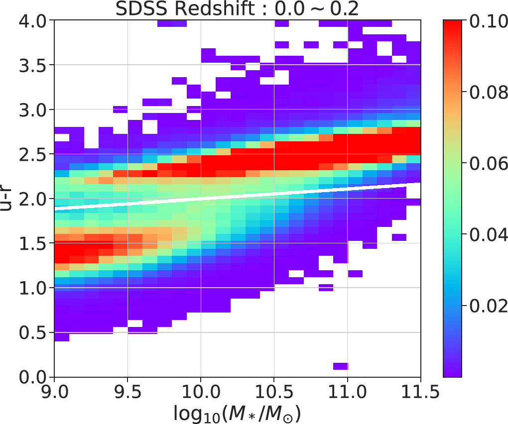
Figure 2. Vmax weighted color distribution in SDSS with the dividing lines used to split galaxies into blue and red. The color bar represents the number of galaxies that are normalized by the total number of galaxies in each stellar mass bin.
Download figure:
Standard image High-resolution image3. Results
3.1. Excess Surface Density Distribution
In this section, we estimate the excess surface density distribution  of different stellar masses and colors for the three redshift ranges according to Table 4. Here, we adopt the jackknife resampling technique (Efron 1982) to evaluate the statistical error. The mean value of
  for galaxies with different stellar masses can be obtained by
The corresponding error is calculated as
Here, Nsub represents the number of jackknife realizations, and  denotes the excess of the projected density for the kth realization. In this work, we adopt Nsub = 50.
To investigate the color distribution of companions, we partition the photometric catalog into red and blue subsamples based on Equation (3). Following the previously outlined steps, we calculate  separately for red and blue galaxies. Considering deblending issues in HSC (Wang et al. 2021a, 2021b), we adopt an inner radius cut of 0.1h−1 Mpc for redshift bins 0.3 < zs
< 0.5 and 0.5 < zs
< 0.7.
separately for red and blue galaxies. Considering deblending issues in HSC (Wang et al. 2021a, 2021b), we adopt an inner radius cut of 0.1h−1 Mpc for redshift bins 0.3 < zs
< 0.5 and 0.5 < zs
< 0.7.
Additionally, we compute  in TNG for the same mass bins and color cut for comparison. The excess surface density distributions
  of red and blue galaxies around central galaxies in each mass bin, measured with PAC in both observations and TNG, are presented in Figures 3–5 for the redshift ranges of 0 < zs
< 0.2, 0.3 < zs
< 0.5, and 0.5 < zs
< 0.7, respectively. In these figures, the red color represents the results for red subsamples, while the blue color represents the results for blue subsamples for both observations and simulations.
of red and blue galaxies around central galaxies in each mass bin, measured with PAC in both observations and TNG, are presented in Figures 3–5 for the redshift ranges of 0 < zs
< 0.2, 0.3 < zs
< 0.5, and 0.5 < zs
< 0.7, respectively. In these figures, the red color represents the results for red subsamples, while the blue color represents the results for blue subsamples for both observations and simulations.
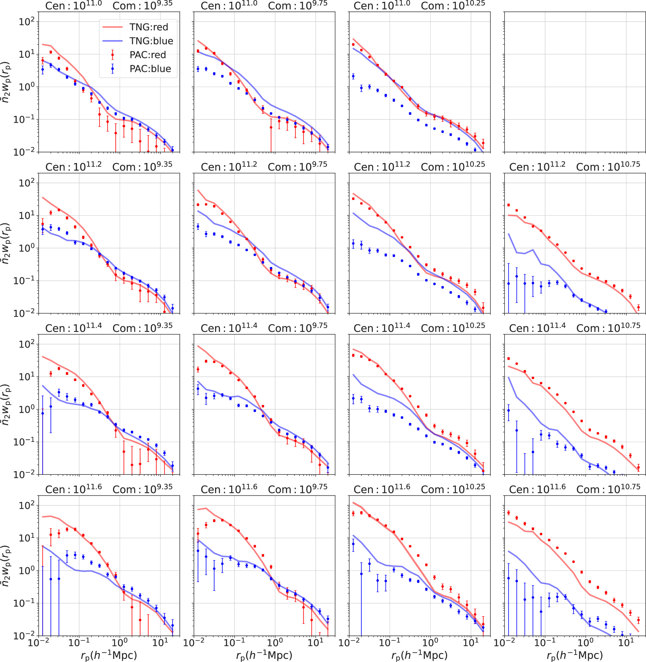
Figure 3. Measurements of  for blue and red subsamples in the redshift range of 0 < zs
< 0.2. The same row represents the results for the same central galaxy mass bin (from top to bottom: [1010.9, 1011.1, 1011.3, 1011.5, 1011.7]M⊙). The four columns from left to right display the results for four distinct mass bins of the photometric sample. The title of each subplot indicates the corresponding central and photometric stellar mass. Colored dots with error bars are the results from observations. Lines are from TNG. Here, the red color corresponds to red subsamples, and the blue color corresponds to blue subsamples for both observations and simulations.
for blue and red subsamples in the redshift range of 0 < zs
< 0.2. The same row represents the results for the same central galaxy mass bin (from top to bottom: [1010.9, 1011.1, 1011.3, 1011.5, 1011.7]M⊙). The four columns from left to right display the results for four distinct mass bins of the photometric sample. The title of each subplot indicates the corresponding central and photometric stellar mass. Colored dots with error bars are the results from observations. Lines are from TNG. Here, the red color corresponds to red subsamples, and the blue color corresponds to blue subsamples for both observations and simulations.
Download figure:
Standard image High-resolution image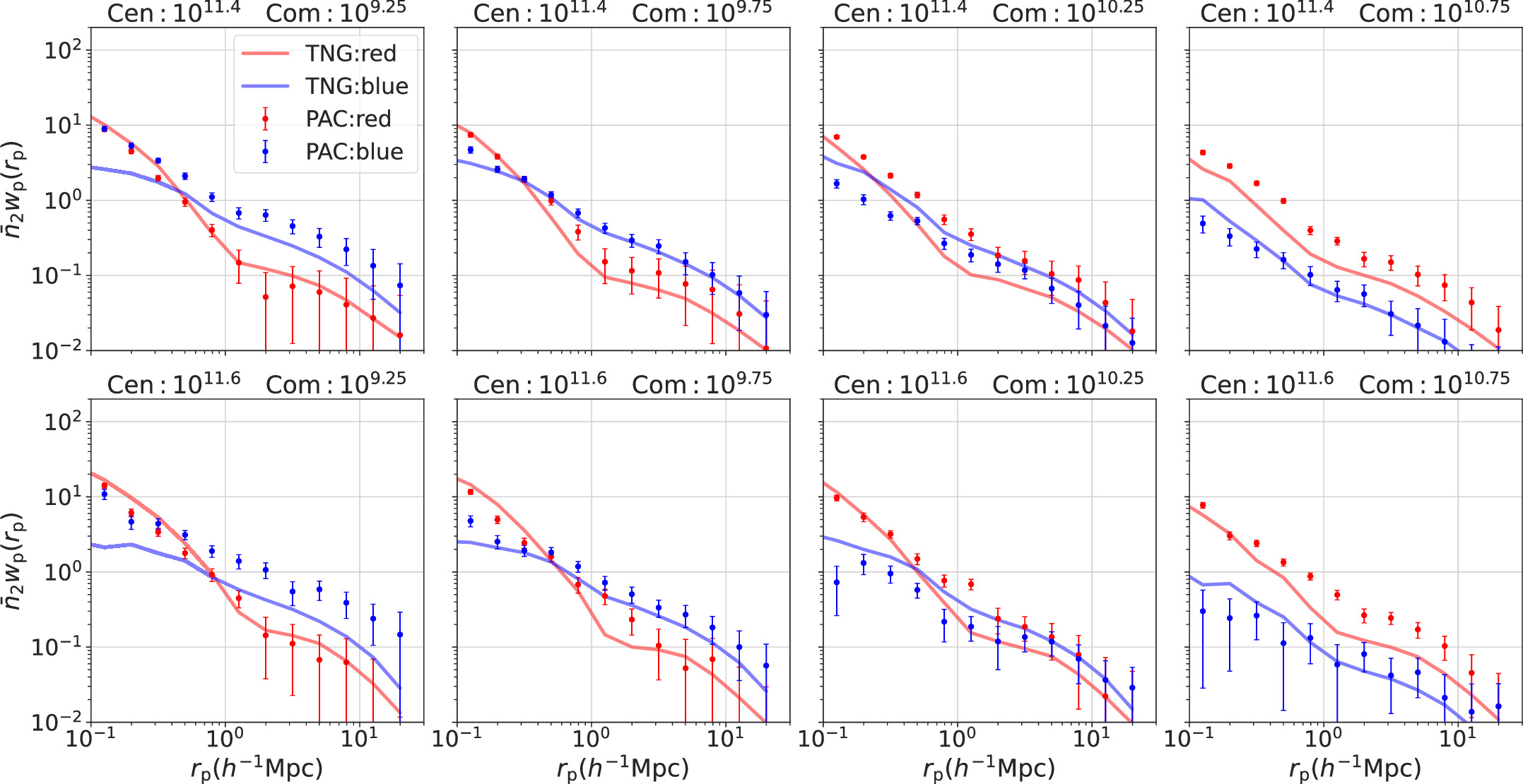
Figure 4. The same as Figure 3 but for redshift range zs = 0.3 ∼ 0.5. The same row represents the results for the same central galaxy mass bin (from top to bottom: Top: 1011.4 M⊙, Bottom: 1011.6 M⊙).
Download figure:
Standard image High-resolution image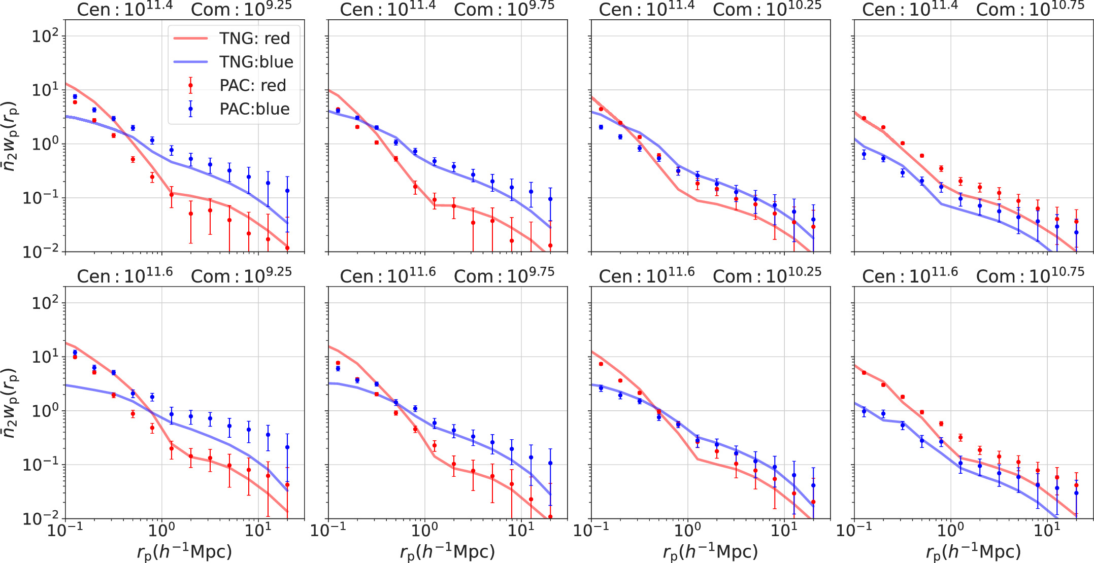
Figure 5. The same as Figure 4 but for redshift range zs = 0.5 ∼ 0.7.
Download figure:
Standard image High-resolution imageIn each redshift bin and mass bin, the  results for red subsamples drop more sharply than blue subsamples within the projected radius rp around 1h−1 Mpc for both observations and simulations, which means the quenched fractions decrease in this range. This shows that galaxies are more likely to be quenched if they are closer to central galaxies, which confirms the effect of environment. Furthermore, as the satellite stellar masses increase in observation, we can find a significant increase in the
  results of red subsamples compared to blue subsamples. This shows the monotonous increase of quenched fraction with stellar mass, which manifests the mass quenching.
3.2. Fraction Profile
To better illustrate the blue and red fraction distributions of galaxies around the centrals, we calculate fractions of  for red and blue subsamples separately. We employ the jackknife resampling technique mentioned earlier to estimate the statistical error of observational data. First, we define the fraction of
  for red or blue subsamples of the kth jackknifed realization as
Here, i represents red or blue subsamples. Then, the mean value of the fraction of  for red or blue subsamples and the corresponding error can be expressed as
The fraction distributions are shown in Figures 6–8. In all these figures, the red color corresponds to the results of the red subsamples, and the blue color corresponds to the blue subsamples. Dots with error bars are for the observations and lines are for TNG.
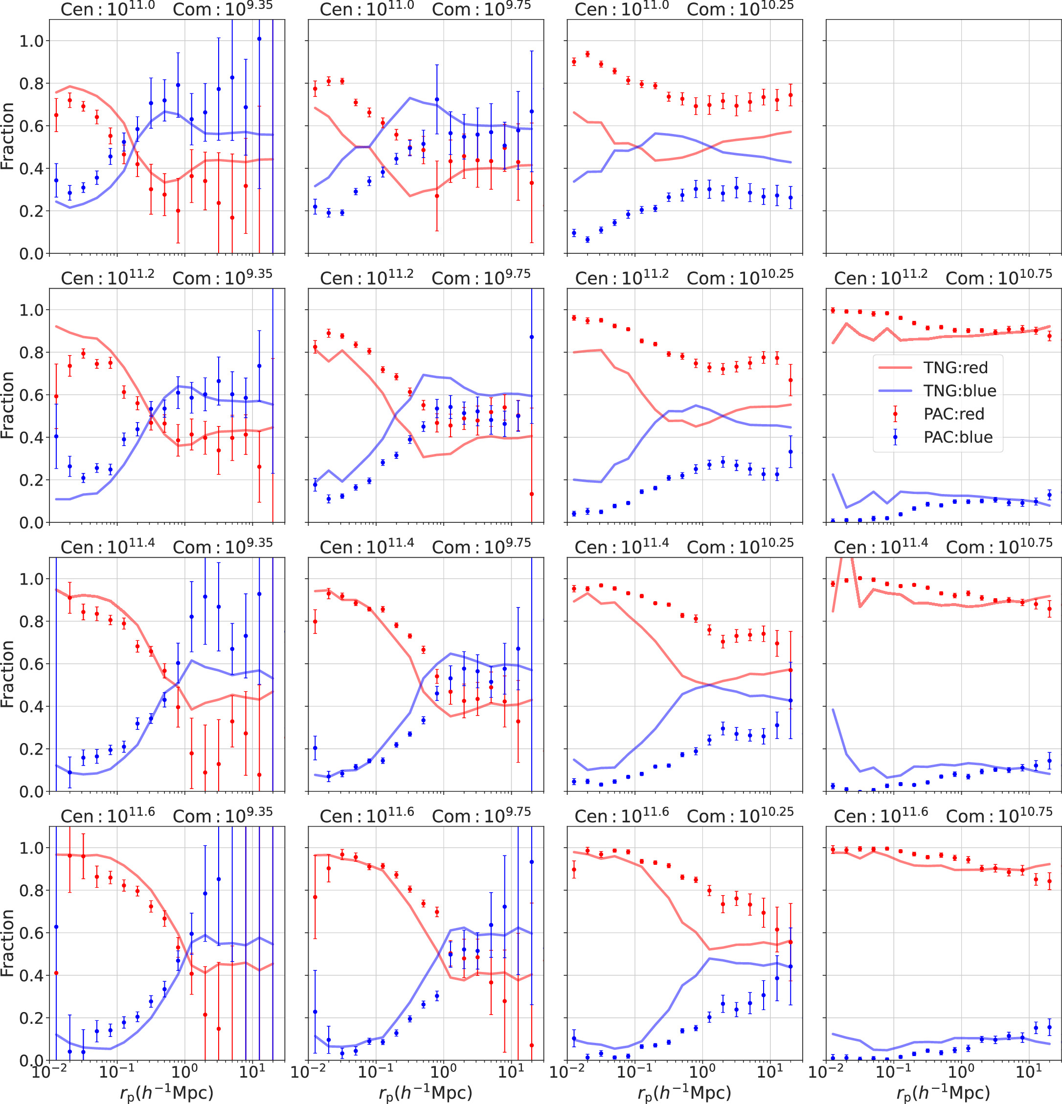
Figure 6. The fraction of  for blue and red subsamples in the redshift range zs
< 0.2. The same row represents the results for the same central galaxy mass bin (from top to bottom: [1010.9, 1011.1, 1011.3, 1011.5, 1011.7]M⊙). The four columns from left to right display the results for four distinct mass bins of the photometric sample. Colored dots with error bars are the results from observations. The lines are from TNG. Here, the red color corresponds to red subsamples, and the blue color corresponds to blue subsamples for both observations and simulations.
for blue and red subsamples in the redshift range zs
< 0.2. The same row represents the results for the same central galaxy mass bin (from top to bottom: [1010.9, 1011.1, 1011.3, 1011.5, 1011.7]M⊙). The four columns from left to right display the results for four distinct mass bins of the photometric sample. Colored dots with error bars are the results from observations. The lines are from TNG. Here, the red color corresponds to red subsamples, and the blue color corresponds to blue subsamples for both observations and simulations.
Download figure:
Standard image High-resolution image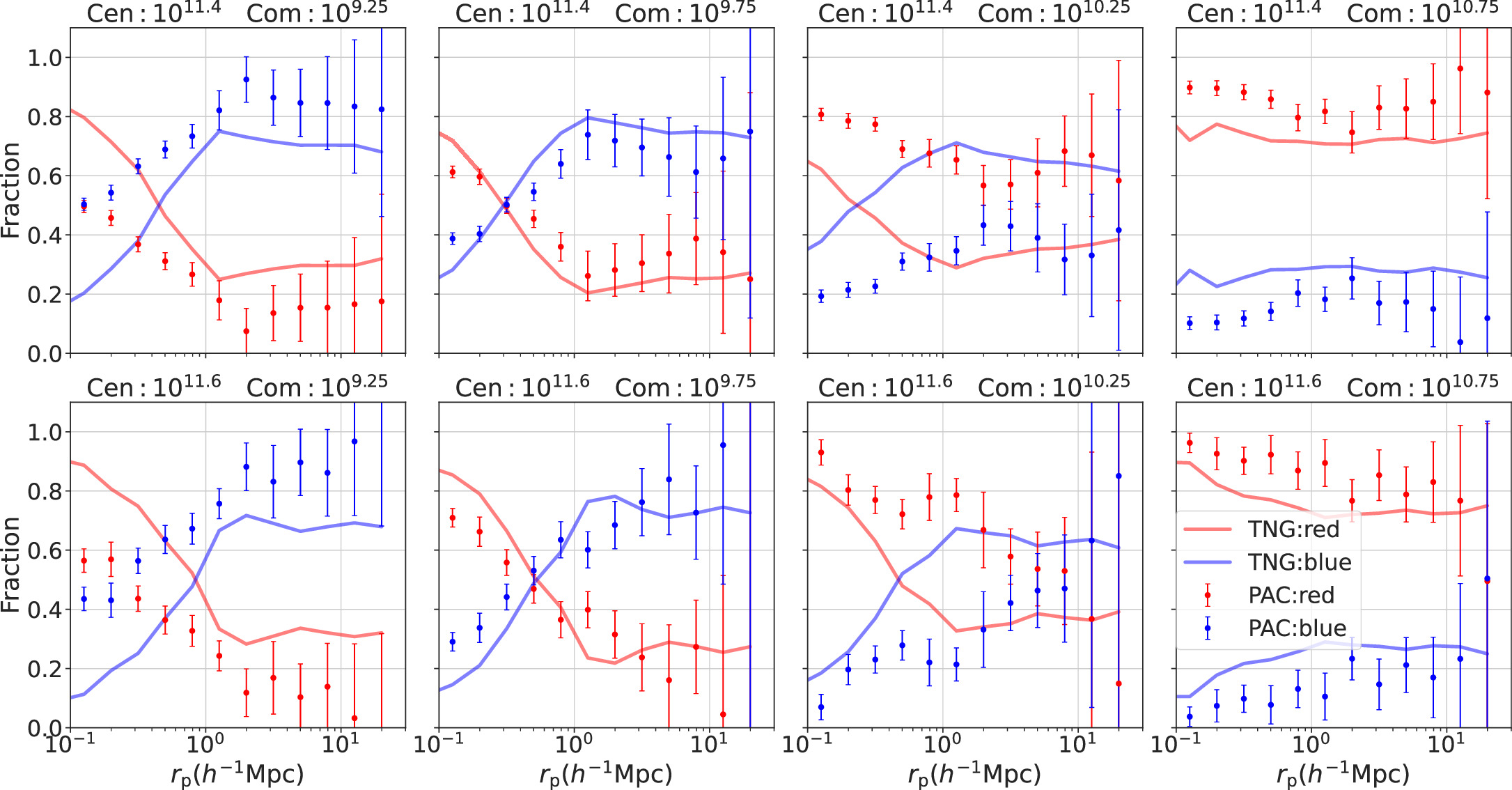
Figure 7. The same as Figure 6 but for redshift range zs = 0.3 ∼ 0.5. The same row represents the results for the same central galaxy mass bin (from top to bottom: Top: 1011.4 M⊙, Bottom: 1011.6 M⊙).
Download figure:
Standard image High-resolution image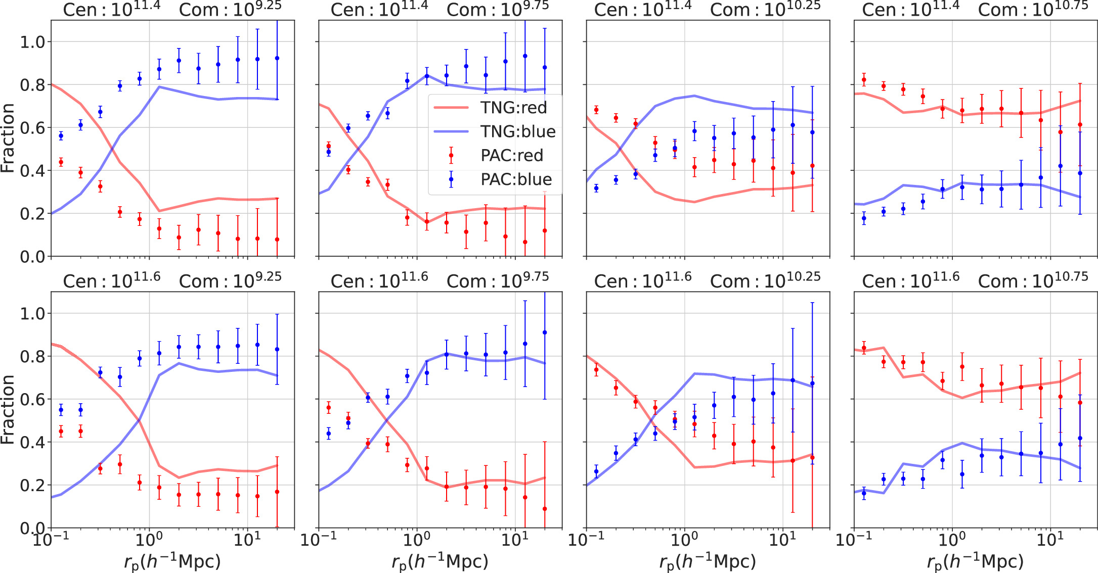
Figure 8. The same as Figure 7 but for redshift range zs = 0.5 ∼ 0.7.
Download figure:
Standard image High-resolution imageFor the radial dependence, in each redshift and mass bin, it is evident that the quenched fractions of galaxies (i.e., the fractions of the red subsamples) decrease with the projected radius rp to the central galaxies for both observations and simulations. This trend reflects the influence of the environment on the star formation of galaxies. Galaxies situated closer to the massive central galaxies, i.e., closer to the center of the massive dark matter halos, are more likely to be quenched. In observations, this trend continues to around 3rvir. At larger distances, the quenched fractions stabilize at nearly constant levels, suggesting that the role of central galaxies (the host halos) in quenching companion galaxies is primarily within 3rvir. This result is consistent with Barsanti et al. (2018), who showed that environmental impact can extend to around 4.5R200. This result is very intriguing, as it is in line with the depletion radius that defines the boundary between the inner growing region of the halo and the depleting environment (Fong & Han 2021; Gao et al. 2023).
Concerning the halo mass dependence, companion galaxies around more massive central galaxies (e.g., 1011.6 M⊙) are more likely to be quenched. This behavior becomes more evident in the total satellite fraction, as shown below. This trend is consistent with Siudek et al. (2022), who found that the fraction of red galaxies increases with the density of the environment. Such a trend may arise from two effects: (1) because more massive halos usually possess more hot gas, ram pressure might be more effective in removing gas around satellite galaxies; and (2) more massive halos have more substructures, leading to increased harassment of companion galaxies.
Regarding the companion stellar mass dependence, as the stellar mass of companion galaxies increases, the red fraction consistently rises at all rp, regardless of whether they are inside or outside the host halos of the spectroscopic central galaxies. At scales larger than 3rvir of the host halos, the red fraction stabilizes at an almost constant value, representing the average value in the Universe. This pattern reflects the fact that quenching depends on stellar mass (mass quenching). In Figures 6–8, it is evident that although the dense halo environment always quenches an additional fraction of galaxies relative to the background mean, the slight increase in the quenched fraction for massive companion galaxies does not imply that the environment is less effective for massive galaxies. Instead, it results from the fact that, due to mass quenching, fewer star-forming galaxies are left that can be influenced by the environment, as we will demonstrate in the next subsection.
3.3. QFE
To better characterize galaxy quenching driven by environmental factors, we compute the QFE that describes the fraction of the star-forming satellite galaxies quenched due to a dense environment as follows:
Here, fq
represents the quenched fraction (i.e., the red fraction obtained in Section 3.2 for simplicity).  is the average quenched fraction of galaxies with the same stellar mass M* at redshift z. In previous studies (e.g., Peng et al. 2010; Balogh et al. 2016; Reeves et al. 2021),
  is chosen as the fraction of quiescent galaxies in the field. However, in this paper, as mentioned in 3.2, massive dark matter halos mainly affect the star formation of their satellites about 3rvir away. Therefore, for each companion mass bin, we select three points located just beyond 2rvir in each central mass bin (e.g., we select a total of six points in two rows of the first column in Figure 8) and calculate the weighted average value for all these points to represent the average quenched fraction
  . The details are as follows:
First, for the companion stellar mass M*,com at redshift zs , we select the three points located just beyond 2rvir in each central mass bin based on Equations (7) and (8), which can be written more explicitly as
Here, k represents the kth jackknifed realization, j represents the three closest points larger than 2rvir, and c is the index of the central mass bins.
Then, we collect all the points in all central mass bins and get the inverse variance-weighted average value of the average quenched fraction  and the error:
Here, C is the number of central mass bins adopted for each companion mass bin, and J = 3, following the definition above for the points around 3rvir. Therefore, C × J represents the total number of points collected for the companion stellar mass bin.
With the quenched fraction results obtained above, we calculate the QFE for different stellar mass bins of central and companion galaxies. With the QFEs, we can quantify the efficiency with which different halo environments quench galaxies of different stellar masses. Based on Equation (9), the σQFE is estimated from the error propagation of the quenched fraction fq and the average quenched fraction  . We also apply the same method to the TNG simulation to get the corresponding results.
Figures 9 and 10 demonstrate the QFE results for different stellar mass bins of central and companion galaxies at three redshifts. For a given central mass (i.e., environment), the QFE is very similar for different satellite galaxies, though there is a rather weak trend that more massive satellites are more easily quenched. This trend, though rather weak, is counterintuitive, as one would expect that the less massive ones are more vulnerable to the dense environment. Although we have not fully understood the cause, we would point out that the quenching efficiency certainly depends on the definition of quenching (the line in Figure 2), and it may take more time for the small ones to be quenched across the definition criterion. For a given companion mass, we can see that the more massive halos are more effective in the quenching even after the scale is normalized by rvir. This can be understood, as we pointed out before, as the ram pressure and the harassment effects are likely more effective in more massive halos. Comparing those of the same stellar bins at different redshifts, we can easily find the quenching efficiency is higher at the lower redshift. As the SHMR changes very slowly in the redshift range of our interest, the corresponding halo mass or radius does change very little (Table 2). The significant change of the QFE with redshift may reflect the fact that the satellite galaxies at low redshift have a longer time to quench in the dense environment than those at higher redshift since the halo accretion rate slows with redshift for a given halo mass effect (Zhao et al. 2003, 2009).
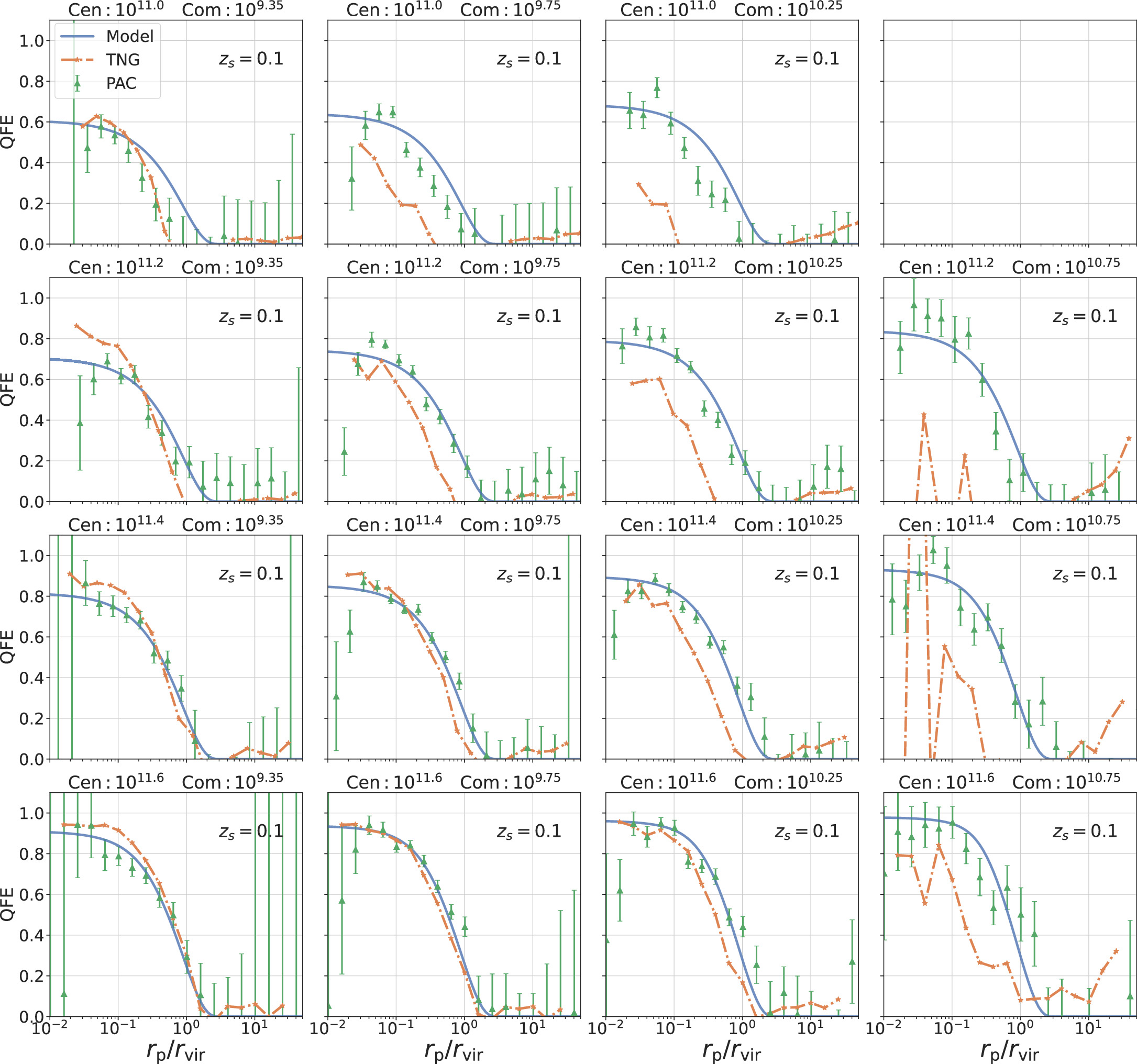
Figure 9. The QFE results of observations (green triangles with error bar), the fitting model (blue lines), and TNG (orange dotted lines) in the redshift range of zs < 0.2. The four columns from left to right show the results for four companion stellar mass bins from 109.2–1011.0 M⊙. The rows from top to bottom display the results for different central stellar mass bins from 1010.9–1011.7 M⊙. Here, we use the mean values to present in each panel. The title of each subplot indicates the corresponding central and companion stellar mass. The mean values of rvir for Jiutian and TNG are listed in Table 2.
Download figure:
Standard image High-resolution image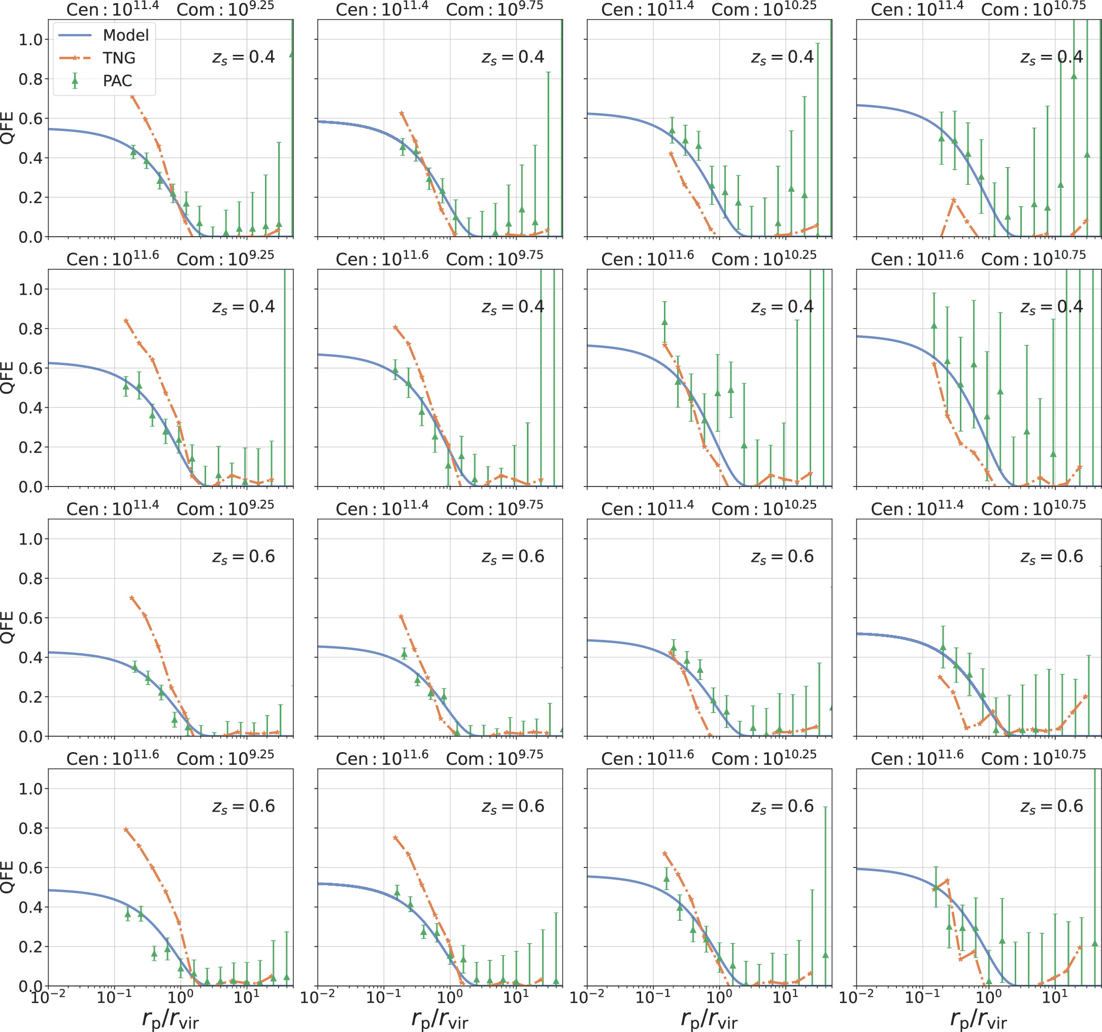
Figure 10. The same as Figure 9 but for different redshift ranges (0.3 < zs < 0.5 and 0.5 < zs < 0.7). The four columns from left to right show the results for four companion stellar mass bins from 109.0–1011.0 M⊙. The rows from top to bottom display the results for these two redshift bins and for different central stellar mass bins from 1011.3 –1011.7 M⊙. The title of each subplot indicates the corresponding central and companion stellar mass.
Download figure:
Standard image High-resolution imageTo summarize, the QFE relies on the halo-centric distance, redshift, mass of host halos, and stellar mass of the companions. Taking into account these dependencies, we propose a fitting model for the QFE that hinges on the companion stellar mass M*, com, the central stellar mass M*, cen, redshift zs , viral radius rvir, viral mass Mvir, and the projected distance rp as follows:
where
Here, we use the function Func to describe these dependencies, and we use an additional limiting function in Equation (14) to guarantee that the QFE is less than 1 for all stellar mass bins. The limiting function effectively maintains the results for small stellar mass bins and places reasonable constraints on large mass bins. It makes sense because we adopt that the satellite galaxies in the innermost region of massive host halos are almost red. Here, we use 3rvir as the critical point according to the definition of the QFE in Equation (9).
In order to construct the fitting model, we use the Markov Chain Monte Carlo (MCMC) sampler emcee (Foreman-Mackey et al. 2013). The fitting results are shown in Figures 9 and 10 as blue lines. Posterior probability density functions (PDFs) of the parameters of our model from the MCMC are shown in Figure 11 and Table 5, χ2/dof = 0.939. All of the parameters are constrained well and the fitting is almost good for all mass bins in all redshift ranges.
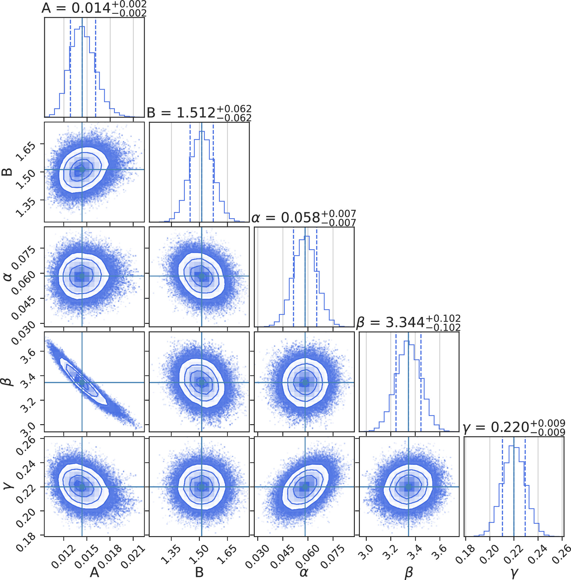
Figure 11. The posterior distributions of the parameters in the fitting model. The 1D PDF of each parameter is plotted as a histogram at the top panel of each column, where the median value and 1σ uncertainty are also labeled. The 2D joint PDF of each parameter pair is shown as a contour with three confidence levels of 68%, 95%, and 99%.
Download figure:
Standard image High-resolution imageTable 5. Posterior PDFs of the Parameters from MCMC with Their 1σ Uncertainties
| Model | A | B | α | β | γ |
|---|---|---|---|---|---|
| Values |

|

|

|

|

|
Download table as: ASCIITypeset image
3.4. Total Satellite Quenched Fraction
We now focus on the total satellite quenched fraction. Satellites are defined as the galaxies within the virial radius rvir of the dark matter halos of the central galaxies.
To calculate the satellite quenched fraction, we need to compute the galaxy number counts within the virial radius rvir for all satellites and for quenched ones, respectively. Thus, we need to drop out the galaxies beyond rvir along the LOS from the projected  . Here, we use the method provided by Jiang et al. (2012) to obtain the number of real satellites and quenched satellites within the distance rvir independently. First, we assume the real space correlation function ξ(r) follows the power-law form
  , then the overall projected correlation function becomes
By fitting the projected radial distribution profile of satellites in the range of 0.1 < rp < 1h−1 Mpc, we can get the correlation length r0 and the power-law index γ. Next, considering wp that comprises two components, one from structures within the virial radius rvir, the other from the correlated nearby structures outside of the virial radius along the LOS, wp can be written as

where

and

By taking the fitting  into Equation (17), we can get wp1 and the ratio wp1(rp)/wp(rp). Afterward, the total number of real satellites within the projected distance rvir can be obtained as
By applying the above steps on  of all samples and the red subsamples separately, we obtain the number of real satellites and quenched satellites accordingly. Finally, we can calculate the quenched fractions for the observations:

We also apply this method to TNG for comparison. Because we obtain the fractions from the surface distribution  , this method could be understood as a 2D method.
To verify the validity of the 2D method, we calculate the satellite quenched fractions in TNG directly and confirm their reliability. The results of the comparison are shown in Appendix B.
Figure 12 shows the satellite quenched fraction for different mass bins and for three different redshift bins. Each panel shows the quenched fractions for the same redshift bin. The results for observation are represented by dots, and those for TNG using the 2D method are represented by solid lines. Different colors represent different central stellar mass bins.
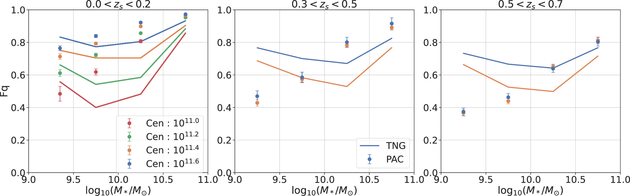
Figure 12. The satellite quenched fractions of observation and TNG for three distinct redshift bins: 0 < zs < 0.2 (left), 0.3 < zs < 0.5 (medium), and 0.5 < zs < 0.7 (right). Colored dots with error bars denote the results from observations. Solid lines denote the TNG 2D method. For both observations and simulations, different colors are used for the corresponding central stellar mass bins: red (1011.0 M⊙), green (1011.2 M⊙), orange (1011.4 M⊙), and blue (1011.6 M⊙).
Download figure:
Standard image High-resolution imageIn the observations, the dependence of the quenched fraction on both central and satellite masses is consistent with what we have mentioned above. The satellite quenched fractions increase monotonously with satellite mass. The quenched fractions also increase with the stellar mass of central galaxies. We also find a redshift evolution of quenched fractions, indicating that galaxies at lower redshift become redder and have higher quenched fractions.
4. Comparison to TNG300-1
To comprehensively assess our observational results, we conduct a detailed comparison with the Illustris TNG300-1 simulation. In this section, we present the key findings of this comparison.
First, examining the excess surface density distribution,  , and the fraction distributions, we observe a clear redshift dependence in both observations and simulations. The red fractions consistently increase with decreasing redshift. Regarding the radial dependence, the red fractions in TNG decrease more rapidly with rp than in observations, indicating a more pronounced increase toward the centers. This may arise from premature stripping of gas around companion galaxies, as also found by Merritt et al. (2020). Concerning the mass dependence, in observations, as companion photometric stellar masses increase, companion galaxies around massive central galaxies exhibit larger red fractions at all rp. This trend persists from 109.0–1011.0
M⊙. However, in TNG, this trend is not consistently observed, with the red fractions of less massive companion galaxies (109.0 ∼ 109.5
M⊙) sometimes exceeding those of the more massive ones (1010.0 ∼ 1010.5
M⊙).
, and the fraction distributions, we observe a clear redshift dependence in both observations and simulations. The red fractions consistently increase with decreasing redshift. Regarding the radial dependence, the red fractions in TNG decrease more rapidly with rp than in observations, indicating a more pronounced increase toward the centers. This may arise from premature stripping of gas around companion galaxies, as also found by Merritt et al. (2020). Concerning the mass dependence, in observations, as companion photometric stellar masses increase, companion galaxies around massive central galaxies exhibit larger red fractions at all rp. This trend persists from 109.0–1011.0
M⊙. However, in TNG, this trend is not consistently observed, with the red fractions of less massive companion galaxies (109.0 ∼ 109.5
M⊙) sometimes exceeding those of the more massive ones (1010.0 ∼ 1010.5
M⊙).
Second, examining the QFE results, we find that both observations and simulations exhibit a clear redshift dependence, with the QFE increasing as redshift decreases. Regarding the influence of the environment, the QFE is notably affected by the central stellar mass in all three redshift ranges, rising with increasing mass in both observations and simulations. This indicates that more massive halos are more effective in quenching. Regarding the dependence on companion stellar masses, the QFE results show a weak trend in observations, where more massive companion galaxies are more likely to be quenched from 109.0 ∼ 1011.0 M⊙. Conversely, the QFE results in TNG exhibit an entirely opposite trend, with the QFE dropping significantly as companion stellar masses increase.
Next, examining the total quenched fraction of satellites, Fq, in both observations and simulations, we observe a redshift evolution where satellite galaxies become redder and exhibit higher quenched fractions at lower redshifts. Regarding the dependence on mass, Fq increases with central stellar mass, and this dependence is more pronounced in TNG than in observations. Concerning satellite stellar mass, Fq monotonously increases in observations, whereas this is not consistently observed in TNG. This suggests that environmental effects do not alter the mass dependence of galaxy color distribution in observations, while environmental effects in TNG appear to be too strong on small satellites.
5. Conclusion
In this paper, we use the PAC method to calculate the excess surface density  of companion galaxies with different masses and colors around massive central galaxies from redshift zs
= 0.7 to the present time. Combining these results, we get the corresponding quenched fractions. Moreover, based on the quenched fraction results, we obtain the QFE and construct a fitting model. Finally, we calculate the satellite quenched fractions for different redshift and mass bins. The results are compared with the Illustris TNG300-1 simulation. Our main results are listed below:
of companion galaxies with different masses and colors around massive central galaxies from redshift zs
= 0.7 to the present time. Combining these results, we get the corresponding quenched fractions. Moreover, based on the quenched fraction results, we obtain the QFE and construct a fitting model. Finally, we calculate the satellite quenched fractions for different redshift and mass bins. The results are compared with the Illustris TNG300-1 simulation. Our main results are listed below:
- 1.Both mass and environment have effects on the quenching of the companion galaxies in observations and simulations. In order to separate them, we use the QFE to quantify the environmental quenching.
- 2.We find that the high-density host halo environment takes effect in quenching the star formation of the companions up to the scale of about 3rvir. We also provide a fitting model of the QFE, which can approximately describe the dependencies on the halo-centric distance, redshift, host halo mass, and companion stellar mass.
- 3.In observations, the quenched fractions Fq of satellites increase monotonously with the satellite's stellar mass, but this trend is not found in TNG, indicating too strong an environmental effect on small satellites in TNG.
In conclusion, mass and environmental quenching can both affect the evolution of companion galaxies. Environmental quenching has wide-ranging effects that can affect the star formation of galaxies up to 3rvir from the halo center. Results from the IllustrisTNG simulation deviate from these observational results, especially for small companions, which may indicate that the galaxy quenching recipes and/or simulation resolutions should be improved. Our fitting model can help test and improve the current galaxy formation models.
In the future, with the deeper and wider spectroscopic and photometric surveys, we can extend our studies to fainter galaxies and higher redshift, taking advantage of PAC.
Acknowledgments
The work is supported by the NSFC (12133006, 11890691), the National Key R&D Program of China (2023YFA1607800, 2023YFA1607801), and the 111 project No. B20019. This work made use of the Gravity Supercomputer at the Department of Astronomy, Shanghai Jiao Tong University. We gratefully acknowledge the support of the Key Laboratory for Particle Physics, Astrophysics and Cosmology, Ministry of Education. We acknowledge the science research grants from the China Manned Space Project under grant No. CMS-CSST-2021-A03. We are grateful for the useful discussions on the galaxy catalog with Wenting Wang. Z.Y. thanks Xiaokai Chen and Jian Yao for their kind help.
The HSC Collaboration includes the astronomical communities of Japan and Taiwan, and Princeton University. The HSC instrumentation and software were developed by the National Astronomical Observatory of Japan (NAOJ), the Kavli Institute for the Physics and Mathematics of the Universe (Kavli IPMU), the University of Tokyo, the High Energy Accelerator Research Organization (KEK), the Academia Sinica Institute for Astronomy and Astrophysics in Taiwan (ASIAA), and Princeton University. Funding was contributed by the FIRST program of the Japanese Cabinet Office, the Ministry of Education, Culture, Sports, Science and Technology (MEXT), the Japan Society for the Promotion of Science (JSPS), the Japan Science and Technology Agency (JST), the Toray Science Foundation, NAOJ, Kavli IPMU, KEK, ASIAA, and Princeton University.
This publication has made use of data products from SDSS. Funding for SDSS and SDSS-II has been provided by the Alfred P. Sloan Foundation, the Participating Institutions, the National Science Foundation, the U.S. Department of Energy, the National Aeronautics and Space Administration, the Japanese Monbukagakusho, the Max Planck Society, and the Higher Education Funding Council for England.
Appendix A: Comparison of the Results
We calculate  using the spectroscopic data directly to compare with the PAC result here. We use the Main sample mentioned before and choose those galaxies located in the continuous region of the NGC. Considering the completeness of the Main sample, we select two satellite samples: galaxies with stellar mass 1010.0
M⊙ < M⋆ < 1010.5
M⊙ at zs
< 0.075 and galaxies with stellar mass 1010.5
M⊙ < M⋆ < 1011.0
M⊙ at zs
< 0.085. We select galaxies with stellar mass 1011.3
M⊙ < M⋆ < 1011.5
M⊙ as the central sample. Then, we obtain
using the spectroscopic data directly to compare with the PAC result here. We use the Main sample mentioned before and choose those galaxies located in the continuous region of the NGC. Considering the completeness of the Main sample, we select two satellite samples: galaxies with stellar mass 1010.0
M⊙ < M⋆ < 1010.5
M⊙ at zs
< 0.075 and galaxies with stellar mass 1010.5
M⊙ < M⋆ < 1011.0
M⊙ at zs
< 0.085. We select galaxies with stellar mass 1011.3
M⊙ < M⋆ < 1011.5
M⊙ as the central sample. Then, we obtain  by calculating the mean number density
  and the PCCF wp(rp) separately. After that, we compare the
  calculated using PAC in the same stellar mass bin at zs
= 0.1. The results of the comparison are respectively shown in Figures A1 and A2. PAC measurements are shown as lines and direct spectroscopic measurements are shown as dots. The misalignment for blue galaxies samples in Figure A2 may be due to the relatively small number of blue galaxies. Except for this, the other results fit remarkably well for all red, blue, and full samples, which gives a direct test of PAC and confirms its practicability.
calculated using PAC in the same stellar mass bin at zs
= 0.1. The results of the comparison are respectively shown in Figures A1 and A2. PAC measurements are shown as lines and direct spectroscopic measurements are shown as dots. The misalignment for blue galaxies samples in Figure A2 may be due to the relatively small number of blue galaxies. Except for this, the other results fit remarkably well for all red, blue, and full samples, which gives a direct test of PAC and confirms its practicability.
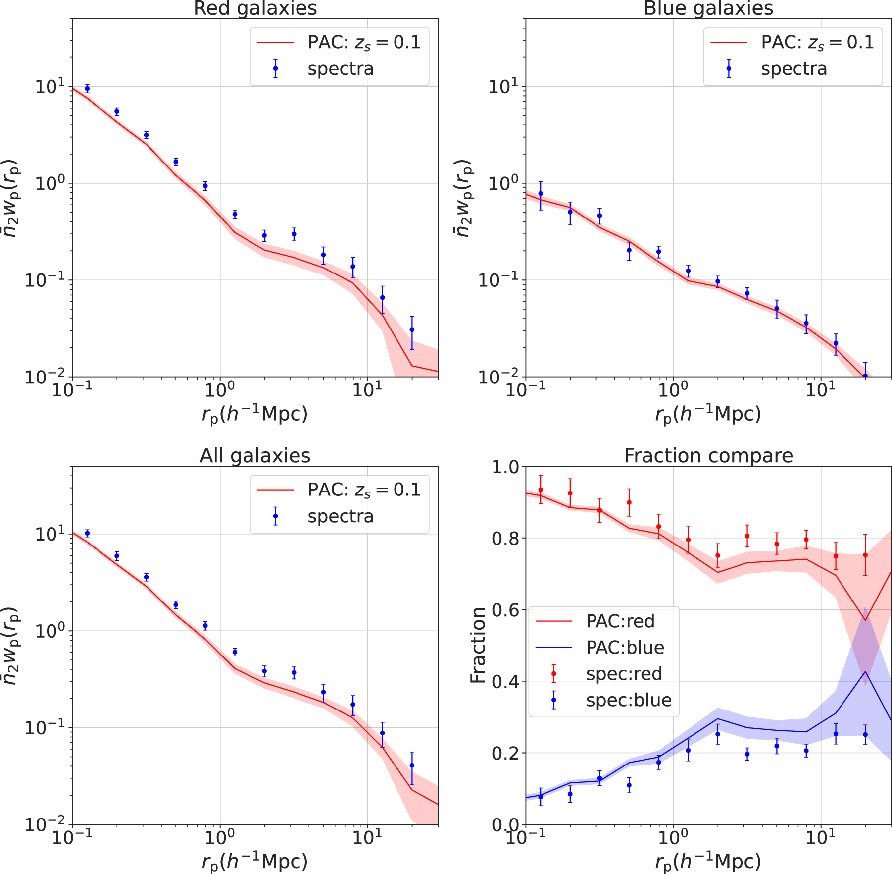
Figure A1. Comparison of  estimated from PAC and the direct calculation from the spectroscopic sample at zs
< 0.075, with a central stellar mass range of 1011.3
M⊙ < M⋆ < 1011.5
M⊙ and satellite stellar mass range of 1010.0
M⊙ < M⋆ < 1010.5
M⊙. The two panels in the top row show the results for red and blue subsamples, respectively. The bottom left panel displays the result for the whole sample. In these three panels, data points represent the results by using spectroscopic directly. Lines with shadows represent the results from PAC. The bottom right panel shows the normalized fraction for red and blue subsamples separately. In this panel, the red line corresponds to the PAC result for red galaxies, the blue line corresponds to the PAC result for blue galaxies, and the dots with error bars correspond to the spectroscopic results.
estimated from PAC and the direct calculation from the spectroscopic sample at zs
< 0.075, with a central stellar mass range of 1011.3
M⊙ < M⋆ < 1011.5
M⊙ and satellite stellar mass range of 1010.0
M⊙ < M⋆ < 1010.5
M⊙. The two panels in the top row show the results for red and blue subsamples, respectively. The bottom left panel displays the result for the whole sample. In these three panels, data points represent the results by using spectroscopic directly. Lines with shadows represent the results from PAC. The bottom right panel shows the normalized fraction for red and blue subsamples separately. In this panel, the red line corresponds to the PAC result for red galaxies, the blue line corresponds to the PAC result for blue galaxies, and the dots with error bars correspond to the spectroscopic results.
Download figure:
Standard image High-resolution image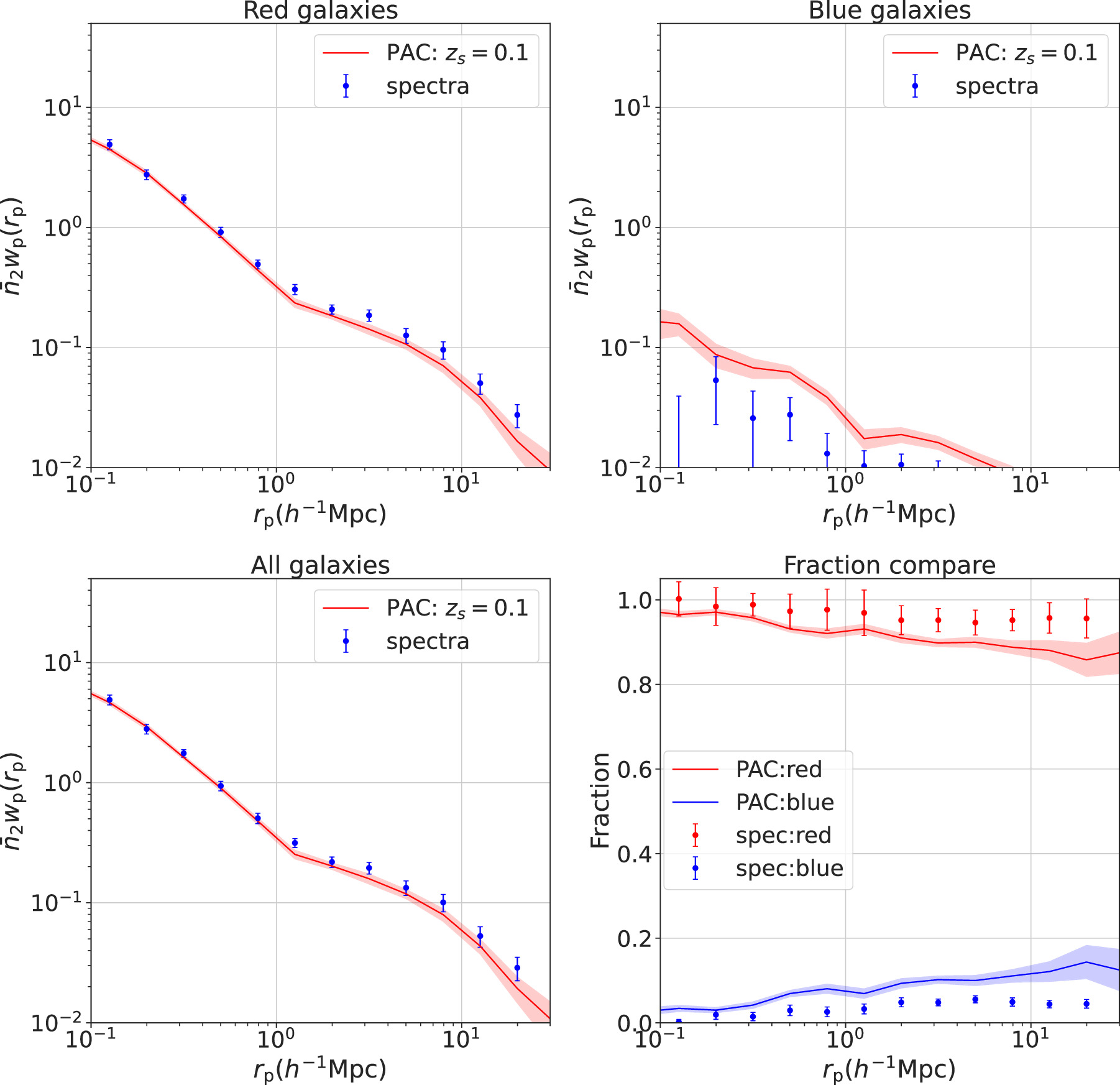
Figure A2. The same as Figure A1 but for the spectroscopic sample at zs < 0.085, with a central stellar mass range of 1011.3 M⊙ < M⋆ < 1011.5 M⊙ and satellite stellar mass range of 1010.5 M⊙ < M⋆ < 1011.0 M⊙.
Download figure:
Standard image High-resolution imageAppendix B: TNG Satellite Quenched Fraction
As mentioned in Section 3.4, to verify the validity of the 2D method, we calculate the satellite quenched fractions in TNG directly. First, we choose the central galaxies and their satellite galaxies in the needed mass bins. Then, we select the satellites within rvir of the central galaxies and get the number of total satellites. After that, we apply Equation (3) to the satellite samples to obtain the quenched satellites. Finally, the quenched fractions can be obtained by dividing the number of red satellites by the total number of satellites. We refer to this method as a 3D method because we are using spatial positions here. The results of the comparison are shown in Figure B1. It can be seen that the two results for the simulations are essentially identical. The relative errors for different mass bins are less than 6.2%, which confirms the correctness of the 2D method.
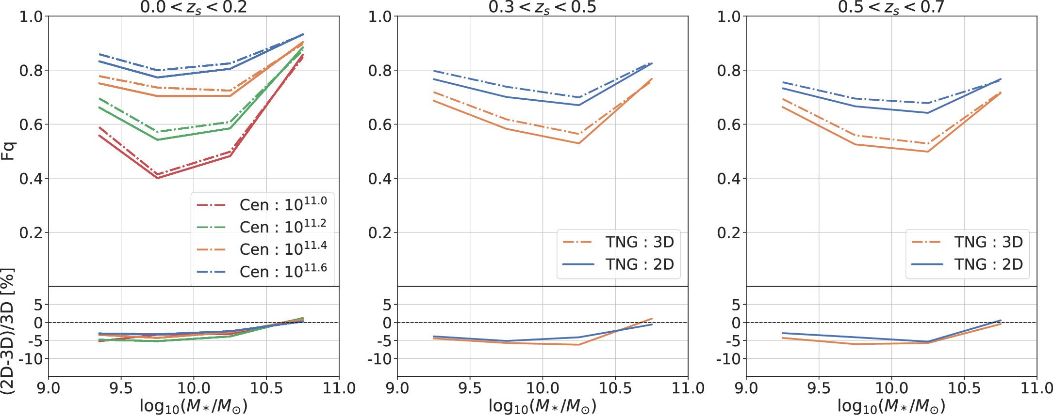
Figure B1. The satellite quenched fraction of TNG for three redshift bins: 0 < zs < 0.2 (left), 0.3 < zs < 0.5 (medium), and 0.5 < zs < 0.7 (right). Solid lines represent the TNG 2D method; dotted lines represent the 3D method. Different colors are used for the corresponding central stellar mass bins: red (1011.0 M⊙), green (1011.2 M⊙), orange (1011.4 M⊙), and blue (1011.6 M⊙).
Download figure:
Standard image High-resolution imageFootnotes
- 6
Throughout the paper, we use zs for spectroscopic redshift and z for the z-band magnitude.
- 7
- 8
- 9
- 10
Because the catalog that contains synthetic stellar photometry does not include the snapshot at zs = 0.6, we choose the snapshot at zs = 0.5 instead.