Abstract
The radio galaxy M87 is well known for its jet, which features a series of bright knots observable from radio to X-ray wavelengths. We analyze the X-ray image and flux variability of the knot HST-1 in the jet. Our analysis includes all 112 available Chandra ACIS-S observations from 2000 to 2021, with a total exposure time of ∼884 ks. We use deconvolved images to study the brightness profile of the X-ray jet and measure the relative separation between the core and HST-1. From 2003 to 2005 (which coincides with a bright flare from HST-1), we find a correlation between the flux of HST-1 and its offset from the core. In subsequent data, we find a steady increase in this offset, which implies a bulk superluminal motion for HST-1 of 6.6 ± 0.9 c (2.0 ± 0.3 pc yr−1), in keeping with prior results. We discuss models for the flux–offset correlation that feature either two or four emission regions separated by tens of parsecs. We attribute these results to moving shocks in the jet, which allow us to measure the internal structure of the jet.
Original content from this work may be used under the terms of the Creative Commons Attribution 4.0 licence. Any further distribution of this work must maintain attribution to the author(s) and the title of the work, journal citation and DOI.
1. Introduction
In extragalactic radio sources, relativistic jets travel hundreds of kiloparsecs from the central engine (Blandford & Rees 1974; Rees 1978; Begelman et al. 1984; Begelman & Cioffi 1989; Bridle & Perley 1984). These prominent jets can be seen in high-luminosity objects, such as 3C 273 (Harris & Stern 1987), PKS 0637-752 (Schwartz et al. 2000), and Pictor A (Wilson et al. 2001), as well as nearby objects like Cen A (Hardcastle et al. 2007) and the radio galaxy M87 (Harris et al. 2003).
M87 is an FR I–type nearby active galactic nucleus (AGN) located at a distance of ∼16.7 ± 0.2 Mpc (Mei et al. 2007). It hosts an extragalactic jet (discovered by Curtis 1918), which features a series of bright knots visible from radio to X-ray. The X-ray knots correlate with optical knots within the jet (Marshall et al. 2002). The cooling time of X-ray-emitting electrons (with γ ∼ 107) will be a few years and optical-emitting electrons will be a few decades. If the emission is synchrotron, the short cooling timescales in the X-ray require that the X-ray-emitting electrons be accelerated locally within the jet (Harris & Krawczynski 2006). Thus X-ray emission regions are ideal probes of energetic particle acceleration processes in jets.
One of the most exciting features of the jet in M87 is the inner knot HST-1, observed at a projected distance of ∼70 pc from the active core (Biretta et al. 1999; Harris et al. 2003, 2006; Perlman et al. 2003). HST-1 is one of the brightest features in the jet and has been studied in detail using multiple telescopes, from radio to optical, near-UV, X-ray, and gamma ray (Biretta et al. 1999; Marshall et al. 2002; Wilson & Yang 2002; Harris et al. 2009; Madrid 2009; Chen et al. 2011; Giroletti et al. 2012). In 2003, a bright X-ray flare was detected from HST-1: the source rose in flux until 2005 and then faded until returning to its prior brightness in 2008 (Harris et al. 2009). Such flares could provide evidence of localized changes and the existence of shock regions in the jets, which can accelerate particles to high energies (Perlman et al. 2011; Imazawa et al. 2021). Analyzing a large set of Chandra observations could therefore trace the physical process and the behavior of the knots in this relativistic jet. The proper motion of the jet and its components has also been a major source of interest and has been studied at a range of spatial scales. For example, the Monitoring Of Jets in Active galactic nuclei with VLBA Experiments (MOJAVE) program using parsec-scale (Homan et al. 2009; Lister et al. 2009) very long baseline interferometry (VLBI) has shown that the FWHM apparent opening angle is ∼69 out from the radio core (Reid et al. 1989; Dodson et al. 2006; Kovalev et al. 2007; Asada et al. 2014) on parsec scales, while observations at larger scales have shown that the dynamic structure varies within the flaring X-ray region of the jet (Cheung et al. 2007; Giroletti et al. 2012). Meanwhile, the Hubble Space Telescope (HST; Biretta et al. 1999; Madrid 2009; Meyer et al. 2013) and the Chandra X-ray Observatory (Snios et al. 2019) have measured the proper motion of HST-1 and other knots along the jet over time. These measurements often reveal significant relativistic motion, where jet features move at velocities close to the speed of light.
Here, we investigate the proper motion of HST-1 in the jet of M87 using a large set of Chandra X-ray images. We find a complex relationship between the flux of HST-1 and its offset from the core, and we develop a toy model to explain the observed behavior.
This paper is organized as follows. In Section 2, we provide the details of the Chandra data reduction. In Section 3, we present the result of our imaging study using spectral modeling, point-spread function (PSF)/MARX ray-tracing simulations, image deconvolution, and radial profiles of the jet. In Section 4, we analyze the apparent motion of HST-1 and present our model of the flux–offset correlation. We compare our results to previous measurements of the proper motion of HST-1 and discuss the implications in Section 5.
Throughout this work we define the photon index Γ as Fε ∝ ε−Γ for photon flux spectral density Fε and photon energy ε; the spectral index is α = Γ − 1.
2. Chandra Data
HST-1 was observed on-axis with the Advanced CCD Imaging Spectrometer (ACIS-S; Garmire et al. 2003) onboard the Chandra X-ray Observatory (Weisskopf et al. 2000) from 2000 to 2021. An example image is shown in Figure 1. For this study, 5 we used 112 ACIS-S pointings with a total exposure time of ∼884 ks. The observations from 2000 and 2018 can be found in Yang et al. (2019), and additional observations are ID 352 (2000), 21457 (2019), 21458 (2019), 23669 (2021), and 23670 (2021). The quality of the data for the focused region varies between the different pointings because the effective PSF is a complicated function of position in the image, the source spectrum, and the exposure time.
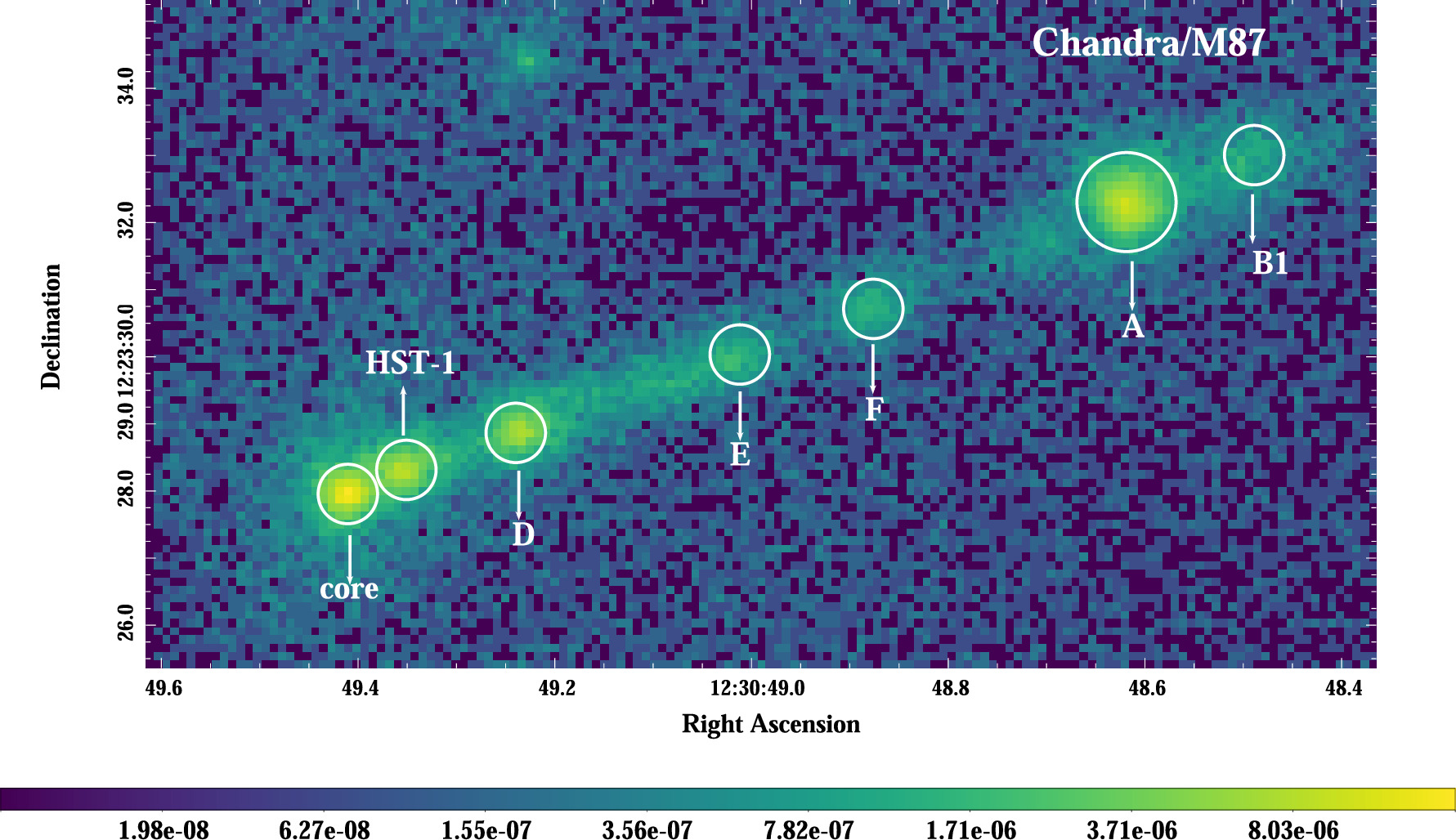
Figure 1. The exposure-corrected 0.4 − 8.0 keV image of the jet in M87, binned to 0.25 px resolution for ObsID 352.
Download figure:
Standard image High-resolution imageThe observational data were reprocessed using the chandra_repro script as per CIAO v4.14 (Fruscione et al. 2006) analysis threads, 6 using CALDB v4.9.7. Pixel randomization and readout streaks were removed from the data during processing and astrometric correction was performed. Point sources in the vicinity of the jet were detected with the wavdetect tool using the minimum PSF method and removed. The wcs_match and wcs_update tools were used to match all the observation IDs (ObsIDs) with reference ObsID 352. All the event and aspect solution files were updated subsequently. For our analysis, we selected photons in the range of 0.4–8.0 keV. Photon counts and spectra were extracted for the source and background regions from individual event files using the specextract script. Spectral fitting was done with the Sherpa 7 package (Freeman et al. 2001). The achieved frame time of all reprocessed observations was 0.4 s (Harris et al. 2006; Yang et al. 2019). The moderate count rate of ≃0.4 counts px−1 s−1 at maximum for HST-1 located in the S3 chip implies a small chance for pileup in the detector (Davis 2001); we included the pileup model when performing MARX ray-tracing simulations (see Section 3.2).
3. Data Analysis
The goal of this work is to use deconvolved images to measure the radial profile of the jet and measure the offset of HST-1 from the core of M87. Although some authors have fit models to data directly for other sources, for HST- 1, we use deconvolved images because it is more straightforward to account for pileup during MARX simulation (Section 3.2) than with direct fitting. Deconvolved images have been used in imaging analysis to study the structure of astronomical sources, for example, to examine the jet’s broadband spectrum and to study the nature of particle acceleration and a correlation between X-ray intensity and optical polarization (Perlman et al. 2003), the proper motion of the pulsar PSR J1741-2054 (Auchettl et al. 2015), the large-scale jet of 3C 273 (Marchenko et al. 2017), and the western hotspot of Pictor A (Thimmappa et al. 2020, 2022). In general, image deconvolution requires a spectrum of the source, modeling of the PSF, and an algorithm to extract the deconvolved images from the data.
3.1. Spectral Modeling
For our spectral analysis, we extracted the source spectrum in each ObsID from a circular region (position: R.A.=12:30:49.3999, decl.=+12:23:28.000) with a radius 3 px (≃15, for the conversion scale 0
492 px−1), and the background was set as a half annulus with an inner and outer radius of 6 and 12 px, respectively; we excluded the half of the annulus that is on the same side of the source as the extended X-ray jet, which is shown in the left panel of Figure 2. The background-subtracted source spectra were fitted assuming a power-law + APEC emission model modified by the Galactic column density NH,Gal = 0.0126 × 1022 cm−2 (HI4PI Collaboration et al. 2016).
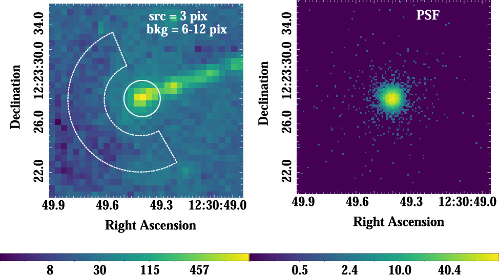
Figure 2. Left panel: ACIS-S image of the source (core+HST-1) in the jet of the M87 radio galaxy, within the energy range 0.4 − 8.0 keV for ObsID 352 (with 1 px binning). The source extraction region for the spectral modeling is denoted by the solid circle (3 px radius) and the background region by a dashed half annulus (6 − 12 px). Right panel: the PSF simulated at 0.25 px resolution for ObsID 352 (as discussed in Section 3.2).
Download figure:
Standard image High-resolution imageA Power-law model with photon index Γ ≃ 2 and vapec model with plasma temperature kT ≃ 0.88 keV provides a reasonable description of the source spectra. It is sufficient in particular for the purpose of the PSF modeling. We note that analogous fits with the Galactic absorption left free returned similar results, with slightly decreased values of NH,Gal, Γ, and kT. Finally, including the jdpileup model in the fitting procedure does not affect the best-fit values of the model parameters as the fraction of piled-up events resulting in a good grade turns out to be very low.
3.2. PSF Modeling
To model the Chandra PSF at the source position (core+HST-1), we used the Chandra Ray Tracer (ChaRT) online tool (Carter et al. 2003) 8 and the MARX software (Davis et al. 2012). 9 For all ObsIDs, the centroid coordinates of the selected source regions were taken as the position. The source spectrum used for the ChaRT tool is the power-law + vapec model in the 0.4–8.0 keV band, as described in Section 3.1. Since each particular realization of the PSF is different due to random photon fluctuations, in each case a collection of 50 event files was made, with 50 iterations using ChaRT by tracing rays through the Chandra X-ray optics. The rays were projected onto the detector through MARX simulation, taking into account all the relevant detector effects, including pileup and energy-dependent subpixel event repositioning. The PSF images were created with a bin size of 0.25 px. An example of the simulated PSF image for ObsID 352 is presented in Figure 2 (right panel).
3.3. Image Deconvolution
We used the Lucy–Richardson Deconvolution Algorithm (LRDA; Lucy 1974), which is implemented in the CIAO tool arestore, to remove the PSF blurring and, in this way, to restore the intrinsic surface brightness distribution of the core and HST-1. This method does not affect the number of counts in the image but only their distribution. The algorithm requires an image form of the PSF, which was provided by our ChaRT and MARX simulations, as described in Section 3.2, and exposure-corrected maps of the source. We obtained the deconvolved images for each ObsID, with 50 different random realizations of the simulated PSF; those 50 deconvolved images (Figure 3, top panel) were then averaged to a single image using the dmimgcalc tool.
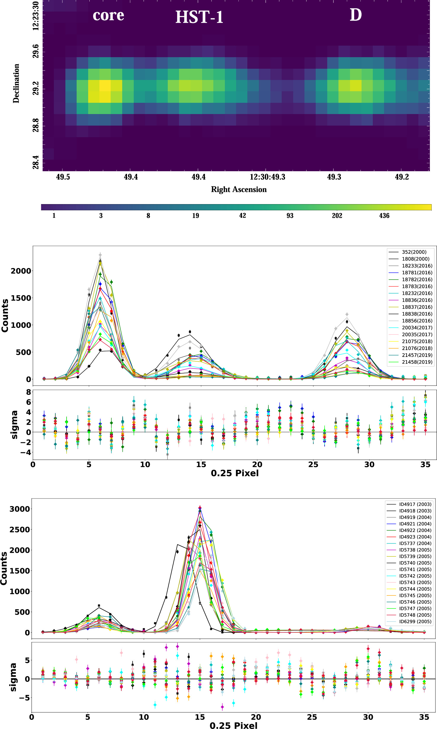
Figure 3. Top panel: the 0.4 − 8.0 keV energy band exposure-corrected deconvolved image of the jet with 0.25 px resolution of ObsID 352. Middle panel: the radial profile of long-exposure (>10 ks) ObsIDs. Bottom panel: the radial profile between 2002 and 2008 (<5 ks) ObsIDs.
Download figure:
Standard image High-resolution image4. Results
4.1. The Radial Profile
We use the 0.25 px or quarter-pixel (qp) deconvolved images described in Section 3.3 to study the radial profiles of the projected jet. The CIAO dmregrid2 tool was used to rotate the deconvolved images. We selected a rectangular region ∼18 × 4 px2 ∼72 × 16 (0.25)px2 around the jet, which includes the core, HST-1, and knot D, as shown in the top panel of Figure 3. The counts were summed for each column of quarter pixels perpendicular to the jet axis to produce the radial profile. We assumed chi2gehrels statistics for the uncertainties. We performed this exercise separately for each ObsID. Based on the counts from the deconvolved images we produced the radial profile of the jet, as shown in Figure 3. The regions of the core, HST-1, and knot D are labeled in the top panel, and the respective radial profiles are shown in the center and bottom panels. The center panel shows the radial profile before and after the flare of HST-1, where observations have longer exposure times (>10 ks). The bottom panel shows the radial profile of HST-1 during the flare between 2003 and 2005, where the HST-1 brightness dominates over the core and exposure times tend to be shorter.
The position of the core, HST-1, and knot D is measured with one-dimensional Gaussian fitting. The model was fit to each ObsID using Sherpa, with the Levenberg–Marquardt method and chi2gehrels statistic. The uncertainties of the parameters are calculated from the confidence method using the conf command in Sherpa, which computes confidence intervals for the given model parameters. Snios et al. (2019) noted that it is difficult to achieve the required astrometric accuracy to measure the proper motion of HST-1 with ACIS, so we opted to perform relative astrometry instead, fitting directly for the offset of HST-1 relative to the core.
The flux of HST-1 was measured from 0.4 to 8.0 keV using the ISIS software package (Houck 2002). For each observation, we model the HST-1 source and background spectra jointly: the background spectrum with a vapec component and the knot spectrum as the sum of a pegpwrlw component and the background model. We use Cash statistics (Cash 1979) and report 90% confidence intervals from our fits. The results are insensitive to the fit method, fit statistic, and the binning of the data. The resulting lightcurve of HST-1 is shown in Figure 4. It is divided into two segments: (i) the period before ∼2008, where the offset and flux rise and fall, and (ii) the period after ∼2008, where the offset steadily rises, implying v/c∼6.6 ± 0.9 (see Section 4.4). Below, we discuss each of these periods in turn.
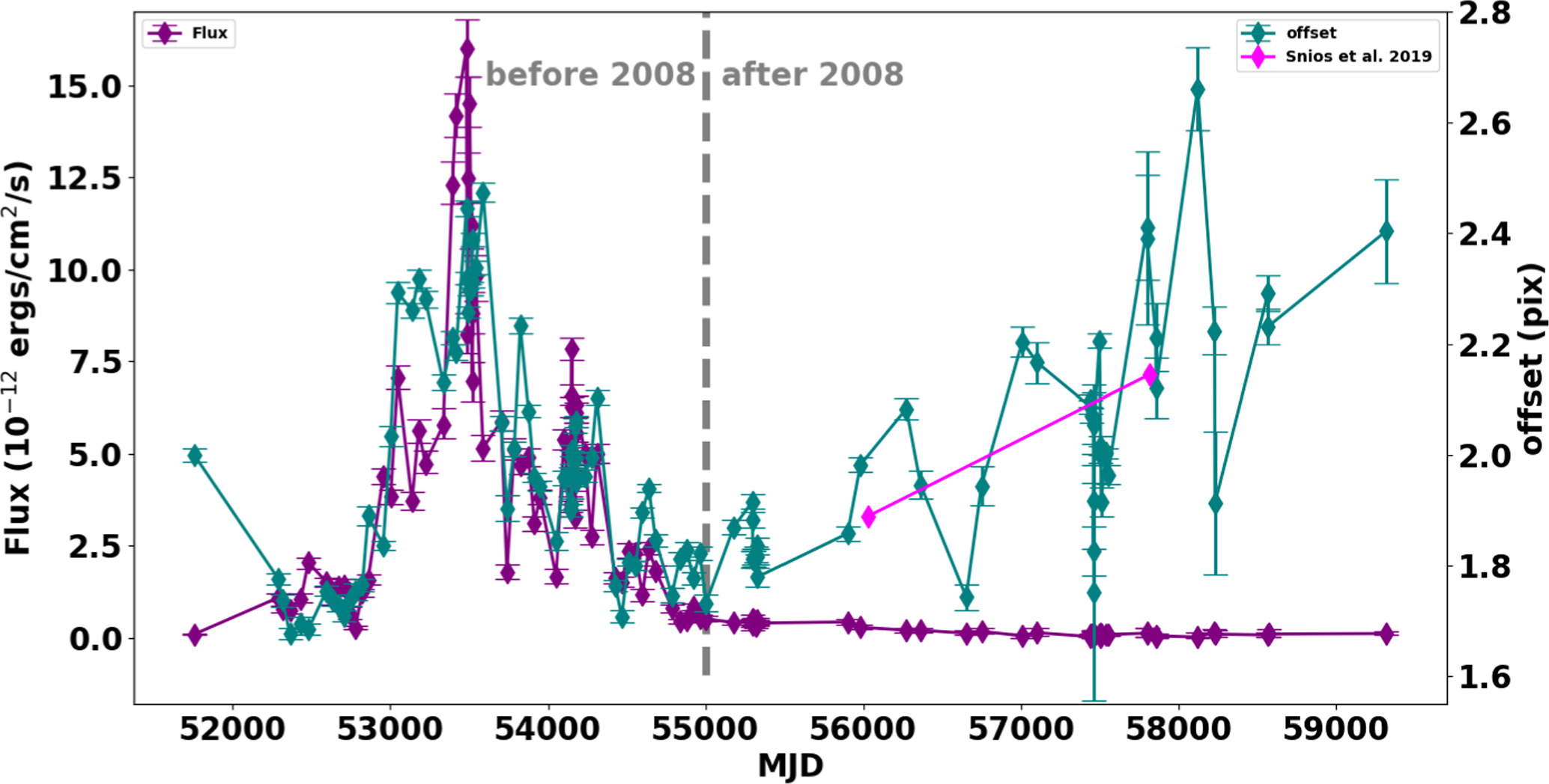
Figure 4. Flux lightcurve and offset of 112 ObsIDs vs. time.
Download figure:
Standard image High-resolution image4.2. The Flux–Offset Correlation before 2008
One of the most interesting features of HST-1 is the bright X-ray flare detected between 2003 and 2008 (Harris et al. 2003, 2006, 2009). Before the flare starts, the separation of HST-1 from the core is ∼70 pc. During the flare time up to ∼2008, the offset is correlated with its flux. Taken at face value, this implies that HST-1 moves away from the core starting in 2002 but then moves back toward the core starting in ∼2005. Since this does not seem physically plausible, it raises a question as to whether the apparent motion of the knot can be attributed to an astrophysical process or an instrumental effect. We consider instrumental effects first, focusing on charge transfer inefficiency (CTI) and pileup (Davis 2001).
(1) We consider the possibility that CTI could instead be responsible for the flux–offset correlation in HST-1. CTI is the inefficient transfer or loss of charge as it is shifted toward the readout. The primary effect of CTI is to reduce measured count rates and reduce the ACIS energy resolution, but it can also smear events in the direction of the readout. 10 Smearing would tend to shift the centroid of the image and might be more noticeable at higher flux. Since it depends on the relative orientation of the source and the readout direction, we searched for a roll-angle dependence in our flux–offset correlation.
A roll-angle dependence of the flux–offset correlation could indicate that CTI is driving the pre-2008 behavior of HST-1. To explore this issue, we checked the roll angles (i.e., 0°–90°, 91°–180°, and 181°–270°) of all observations from 2000 to 2008. For each roll-angle interval, we performed three linear regression analyses in Python: (1) using curve_fit, (2) using curve_fit with errors sampled by Monte Carlo simulation (100,000 iterations), and (3) using the LINMIX package, a Bayesian approach to linear regression. Fitted plots are shown in Figure 5 for the curve_fit method. The fitted and simulated values of the slopes are given in Table 1.
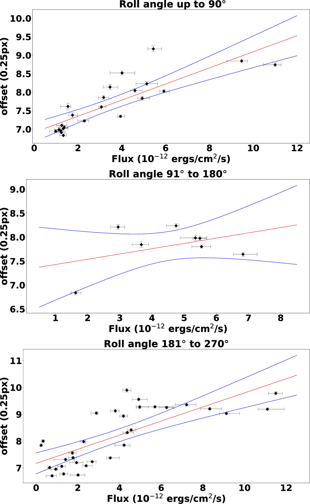
Figure 5. The linear regression model for the flux vs. offset of the roll angles (90°, 180°, and 270°) during the period 2000–2008. The model is shown in a red line, while the blue line shows a 95% confidence region.
Download figure:
Standard image High-resolution imageTable 1. Slope of the Flux–Offset Correlation for the 0°–90°, 91°–180°, and 181°–270° Data Sets
| Method | 90° | 180° | 270° |
|---|---|---|---|
| Curve fit | 0.22 ± 0.03 | 0.11 ± 0.10 | 0.26 ± 0.04 |
| Monte Carlo | 0.220 ± 0.006 | 0.109 ± 0.001 | 0.262 ± 0.007 |
| Linmix | 0.22 ± 0.03 | 0.11 ± 0.17 | 0.26 ± 0.04 |
Note. Units are qps per 1 × 10⁻¹²erg cm−2s−1 = 1 × 10¹² qp cm2s erg−1. Here, qp is a quarter-pixel.
Download table as: ASCIITypeset image
In Table 1, the error bars for the Monte Carlo method are much smaller than the error bars for the other method, which means that the uncertainty in the other fits is primarily due to scatter in the data. If there is no roll-angle dependence in the flux–offset correlation, the results in Table 1 should be consistent with a constant slope. Based on the value of the slope for different roll angles, we considered a constant model M in the range 0.01 − 0.40 × 10¹² qp cm2 s erg−1. We then calculated the respective χ2,

where Di is the slope of the linear regression model with the LINMIX method for 90°, 180°, and 270° and σi is the uncertainty of the slopes. We found that χ2 is minimized at M = 0.23 with a value χ2=1.13. The corresponding p-value for a χ2 distribution with 2 degrees of freedom is 0.56, which indicates that there is no strong evidence of a roll-angle dependence in the flux–offset correlation. Therefore, we conclude that there is no evidence that CTI plays a significant role in the flux–offset correlation.
(2) When two sources are close together, pileup can occur between them, where their PSFs overlap. The loss of photons between these regions can increase their apparent separation in a way that depends on flux. Therefore, we simulate images of two closely spaced sources (separated by 7 qp), one at constant flux and one at a wide range of fluxes, to quantify the effect of pileup on the apparent offset between the two sources. We follow the procedure described in Section 3 to produce radial profiles of our simulations (accounting for pileup during the MARX simulations) and measured the apparent offsets using 1D Gaussian models. We perform a linear regression analysis for the resulting offset and simulated flux of the HST-1, as shown in Figure 6. The slope is 0.073 ± 0.007 × 10¹² qp cm2 s erg−1. We compare this value with our real observational value of HST-1, which at 0.161 ± 0.015 × 10¹² qp cm2 s erg−1 is statistically inconsistent with the simulated flux dependence described above. This result shows that the flux–offset correlation in HST-1 is partially but not fully explained by pileup (see Section 4.3.2). Accounting for pileup in our models of the flux–offset correlation is essential for understanding the structure of HST-1.
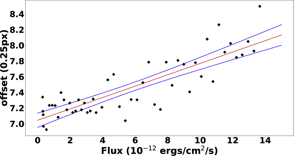
Figure 6. Linear regression model for the offset vs. simulated flux of HST-1.
Download figure:
Standard image High-resolution image4.3. The Flux–Offset Model
Since the apparent motion of HST-1 could not be solely explained by the pileup model (see Section 4.3.2), we consider a toy model to explain why the position of the knot could correlate with flux, appearing to move away from and then toward the core at highly superluminal speeds. Our model supposes that HST-1 is composed of multiple emitting regions and that the centroid position of the knot reflects their relative fluxes. That is, we assume the position of HST-1 in our data is the flux-weighted centroid of its components. The model is illustrated in Figure 7, containing two unresolved emitting regions: the baseline position of HST-1 with constant flux F0 is shown in black, while a variable region with flux f(t) is shown in red a distance d downstream. The arrows show the respective emission regions within HST-1. The top panel is a visualization of the shift of the centroid (whose location is illustrated with a small arrow). As f(t) changes, the apparent position of the knot shifts as well.
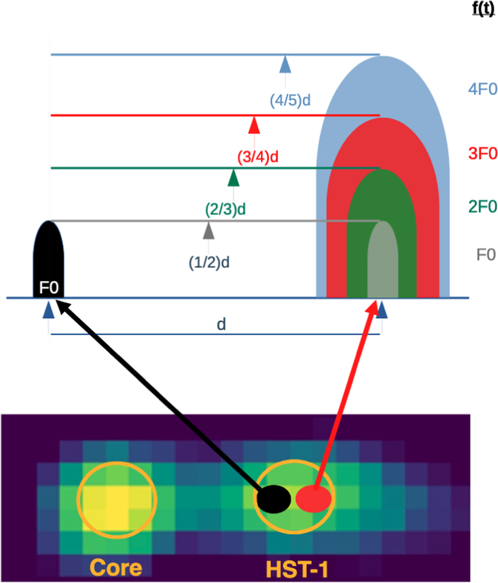
Figure 7. Bottom panel: deconvolved image of core and HST-1 in M87, with two emission regions (black and red circles) shown inside HST-1. Top panel: cartoon for Model 1 showing how relative variations in these emitting regions can lead to an apparent shift in the centroid of HST-1 (arrows). This cartoon connects the internal structure of the jet, the separate variation of flux, and the apparent position of HST-1.
Download figure:
Standard image High-resolution imageIn this model (i.e., Model 1), the offset O(t) of HST-1 from the core is given by

where D is the initial offset of HST-1 before the flare and C(t) is the centroid position, a is the slope value from the flux–offset models to account for pileup, and f(t) is the variable flux. The centroid position is equal to the ratio of the variable flux and total flux times the downstream separation d:

The best-fit position of HST-1 is a good approximation to the flux-weighted centroid when d is small (by our estimates ≤1.5 times the FWHM of the deconvolved sources or ∼5 qp). We consider the upstream region to be stationary but allow the downstream component to move with velocity Vws after time t0. Since Vws was poorly constrained by our data, we fixed it at the previously measured speed of HST-1 (6.4 c=5.56×10⁻⁴qp/day; see Section 4.4 and Snios et al. (2019)). This downstream region may be analogous to a working surface in a jet, where ejecta collide and form internal shocks. These have been studied in detail by Cantó et al. (2000) and Mendoza et al. (2009). These analyses indicate that the lightcurve of a working surface may have a rapid rise and an exponential decay (Cantó et al. 2000; Figure 2). Coronado et al. (2016) applied these models in a detailed study of the flaring lightcurve of HST-1. Nakamura et al. (2010) developed relativistic magnetohydrodynamic (MHD) models of the shocks in the jet of M87.
For our fit model for the lightcurve of HST-1, we approximate the exponential rise/decay lightcurve of a working surface as

where A is the amplitude, t is the time, and τ1 and τ2 are fall and rise times, respectively. We link the flux and offset models in Equations (3) and (4) while joint fitting to measure the common parameters using the Sherpa package. Based on these equations we can fit for the separation between the two emission regions inside HST-1. The above model is implemented in Sherpa and fitted to the lightcurve and offset of HST-1, as shown in Figure 8 (left). The resulting parameters of the models are given in Table 2. We used Model 1 to measure the separation between the two emission regions inside HST-1 and the initial offset from the core. From Model 1, in the beginning of the flare (MJD 52800 ± 20) the initial offset from the core is D = 7.07 ± 0.01 qp ≃76.5 ± 0.1 pc, and the separation between the two emitting regions inside HST-1 is d= qp ≃
qp ≃ pc. For Model 1, we neglect pileup, but we account for it in Model 1A by setting a = 0.073 × 10¹²qp cm2s erg−1 in Equation (2) (i.e., drawing on our MARX simulations from Section 4.2). The resulting fit parameters are similar overall, but the initial offset and downstream separation (D and d) are both reduced a little as expected.

Figure 8. Left: joint fits of Model 1A (i.e., Equations (4) and (2)) to flux (purple X) and offset (green pentagon) of HST-1. Right: joint fits of Model 2A to flux (teal star) and offset (magenta square) of HST-1.
Download figure:
Standard image High-resolution imageTable 2. The Resulting Parameters of the Models
| Flares | Parameters | Symbol | Model 1 | Model 1A | Model 2 | Model 2A | Model 2B | Model 2C |
|---|---|---|---|---|---|---|---|---|
| Main flare | Flux | Fo | 1.08 ± 0.01 | 1.19 ± 0.02 | 1.00 ± 0.03 | 0.80 ± 0.02 | 0.74 ± 0.03 | 0.85 ± 0.02 |
| Amplitude | A1 | 800 ± 300 | 850 ± 310 | 660 ± 700 | 80 ± 23 | 31 ± 8 | 28 ± 7 | |
| Start Time | to1 | 52800 ± 20 | 52750 ± 20 | 52800 ± 40 | 52925 ± 9 | 52968 ± 4 | 52975 ± 3 | |
| Fall Time | τ1 | 211 ± 7 | 238 ± 7 | 201 ± 20 | 118 ± 14 | 130 ± 16 | 126 ± 16 | |
| Rise Time | τ2 | 1200 ± 170 | 1300 ± 160 | 1200 ± 400 | 208 ± 30 | 85 ± 17 | 70 ± 13 | |
| Offset | D | 7.07 ± 0.01 | 6.84 ± 0.01 | 6.95 ± 0.01 | 6.94 ± 0.01 | 6.93 ± 0.01 | 6.96 ± 0.01 | |
| Distance | d1 |

| 1.45 ± 04 | 1.83 ± 0.06 | 2.02 ± 0.06 | 1.75 ± 0.08 | 2.20 ± 0.06 | |
| Slope | a | 0 | 0.073 | 0 | 0.073 | 0.123 ± 0.008 | 0.092 ± 0.008 | |
| Subflare 1 | Amplitude | A2 | ⋯ | ⋯ | 30 ± 5 | 133 ± 106 | 112 ± 99 | 106 ± 59 |
| Start Time | to2 | ⋯ | ⋯ | 53400 ± 4 | 53276 ± 35 | 53265 ± 43 | 53288 ± 25 | |
| Fall Time | τ1 | ⋯ | ⋯ | 86 ± 9 | 145 ± 13 | 167 ± 19 | 142 ± 9 | |
| Rise Time | τ2 | ⋯ | ⋯ | 22 ± 6 | 233 ± 134 | 251 ± 160 | 184 ± 84 | |
| Distance | d2 | ⋯ | ⋯ | 2.60 ± 0.06 | 1.56 ± 0.03 | 1.06 ± 0.07 | 1.76 ± 0.00 | |
| Subflare 2 | Amplitude | A3 | ⋯ | ⋯ | 20 ± 10 | 48 ± 53 | 40 ± 42 | 38 ± 37 |
| Start Time | to3 | ⋯ | ⋯ | 54000 ± 50 | 54000 ± 50 | 54001 ± 50 | 54006 ± 44 | |
| Fall Time | τ1 | ⋯ | ⋯ | 150 ± 20 | 143 ± 20 | 154 ± 21 | 144 ± 18 | |
| Rise Time | τ2 | ⋯ | ⋯ | 100 ± 100 | 214 ± 180 | 204 ± 170 | 180 ± 145 | |
| Distance | d3 | ⋯ | ⋯ | 0.95 ± 0.04 | 0.66 ± 0.03 | 0.37 ± 0.05 | 0.75 ± 0.02 | |
| red.χ2 |

| 40.029 | 33.698 | 22.940 | 20.263 | 20.145 | 20.804 | |
Note. Unit of flux and amplitude is 10−12erg cm−2 s−1; unit of start time, fall time, and rise time is days; unit of offset and distance is qp; and slope is 1012qp cm2s erg−1. Model 1 and Model 2 are given before adding a value. Model 1A and Model 2A are the best fit when a is fixed at 0.073. Model 2B is the best fit of Model 2 when a is set free. Model 2C is the best fit of Model 2 when a is allowed to vary within its 3σ range (see text for details).
Download table as: ASCIITypeset image
In Figure 8 (left), the model flux lightcurve increases gradually and then decays exponentially, in broad agreement with the data. The offset model rises suddenly but decays gradually. We attribute the larger scatter in the residuals to scatter in the offset itself. However, there are two time periods (MJD 53500 and 54250) where the model does not match the observed flux. This period of time indicates possible additional flares and the discrepancy. This might be solved by adding additional flaring components into the model.
4.3.1. Models with Pileup and Centroid Shifts
To account for the multiple emitting regions (subflares) inside HST-1, we extended our model (i.e., Model 2) of the flux and offset. In Model 2, the flux is the sum of a constant and three flare components, while the offset at any time is given by D plus the centroid position of the four emission regions. Model 2 includes additional parameters compared to Model 1 (seven parameters), as shown in Table 2. Similar to Models 1 and 1A, we included the pileup term from Equation (2) and set a to 0.073 for Model 2A to vary freely for Model 2B and to vary within its 3σ range for Model 2C. For Model 2A, 2B, and 2C, the parameters are given in Table 2. For example, in Model 2A at the beginning of the flare (MJD 52925 ± 9), the measured initial offset (baseline position) from the core is D = 6.94 ± 0.01 qp ≃75.1 ± 0.1 pc, and the separation between the main flare region and the baseline of HST-1 is d1=2.02 ± 0.06 qp ≃21.9 ± 0.6 pc. The first additional flare (subflare 1) occurs ∼351 days later at a distance of d2 = 1.56 ± 0.03 qp ≃16.9 ± 0.3 pc from the baseline position of HST-1. The separation is smaller than that of the main flare. The second flare (subflare 2) is closer (d3 = 0.66 ± 0.03 qp ≃4.0 ± 0.3 pc) but takes place later at MJD 54000 ± 50.
Figure 8 (right) shows Model 2A for comparison to Model 1A. The lightcurve of Model 2A rises at MJD 53500 due to the effect of subflare 1. Later, the model flux rises slightly around MJD 54200 due to subflare 2 and then comes back to the baseline of HST-1 by MJD 55000. The offset model curve is similar to the curve in Model 1A, with additional increases in offset due to the effect of subflare 1 and subflare 2. Among these three models, we prefer Model 2A, which has the most realistic value of a given our MARX simulations in Section 4.2.
4.3.2. Pileup-only models
Based on the likely contribution of pileup to the offset, we also consider pileup-only models, where the centroid position C(t) = 0 appears in Equation (2). In the pileup-only model, the value of a determines how the offset changes with the flux of HST-1. As with Model 2, we set the pileup term a to 0.073 for Model 3A to vary freely for Model 3B and to vary within its 3σ range for Model 3C. Models 3A and 3C do not fit the data nearly as well as models with centroid shifts, but Model 3B provides the best overall fit with reduced χ2=20.070. The best-fit pileup parameter in this model is a=0.292 ± 0.006 × 10¹²qp cm2s erg−1. However, such a strong pileup effect is difficult to reproduce in MARX simulations. In principle, a might be larger for sources that are closer together and have more PSF overlap between them. Indeed, when we decrease the separation to 5 qp in our MARX simulations from Section 4.2, we find that a increases to 0.087 ± 0.009 × 10¹²qp cm2s erg−1. However, this increase appears to be bounded: when we decrease the separation to 3 qp, the value of a drops by a factor of 10 to 0.008 ± 011 × 1012qp cm2s erg−1 (likely because the two sources effectively merge into a single source). Therefore, we cannot reasonably attribute such a large value a = 0.292 ± 0.006 × 10¹²qp cm2s erg−1 from Model 3B to pileup between the core and HST-1. Hence, we believe that the pileup-only Model 3B, despite providing the best fit to the data, is unphysical, and we reject it in favor of Model 2A.
4.4. Superluminal Motion after 2008
After 2008, we found no correlation between the offset and the flux. Instead, there is a steady increase in the offset from 2009 to 2021, as shown in Figure 9. We performed a linear regression analysis for the offset versus time in Python using the curve_fit method. With this model, we measured the bulk speed (v/c) of HST-1. The slope is 0.00051 ± 0.00007 (qp/day) or 1.3 ± 0.2 × 10−4 px/day, which corresponds to a measured superluminal speed of 6.6 ± 0.9 c or 2.0 ± 0.3 pc yr−1. Our measured value is consistent with previously measured values of the velocity from HST and Chandra (e.g., Biretta et al. 1995, 1999; Meyer et al. 2013; Snios et al. 2019).
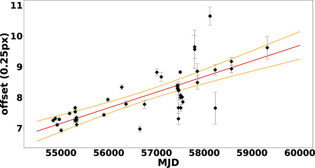
Figure 9. Linear regression model for the offset of HST-1 vs. time during the period between 2009 and 2021 (see Section 4.4).
Download figure:
Standard image High-resolution image5. Discussion and Conclusion
We have collected 112 pointings of Chandra ACIS-S data for the M87 radio galaxy between 2000 and 2021 with a total exposure time of ∼887 ks and used them to perform image analysis of HST-1. We use astrometric and pileup corrections and PSF/MARX simulations to produce 0.25 px deconvolved images. The resulting deconvolved images are used to study the radial profile of the X-ray jet and to measure the relative separation between the core and HST-1. Any proper motion of HST-1 should produce a shift from the core. Our novel relative astrometry makes it possible to measure the proper motion of HST-1 in a large ACIS data set, even when the absolute astrometry of ACIS is not sufficient for the task (Snios et al. 2019).
Before 2008, we found a correlation between the flux of HST-1 and its offset from the core (see Figure 4 from MJD 53000 to 55000), which coincides with a bright flare from HST-1. As the flare flux rises and falls, HST-1 appears to recede from and then approach the core. We have developed a toy model to describe both offset and flux that accounts for physical changes in the flux and position of the knot as well as pileup (Section 4.2).
In our model, we attribute changes in flux to additional variable emission regions inside the jet, similar to the working surfaces described in, e.g., Cantó et al. (2000), Mendoza et al. (2009), Cabrera et al. (2013), and Coronado et al. (2016). As these variable fluxes change, the apparent centroid of HST-1 appears to shift.
Mathematical models were first applied to knots in relativistic jets by Rees (1966), resulting in the measurement of superluminal motion. Since then, analytical and numerical methods have been applied to the internal working surfaces in jets for different sources. Cantó et al. (2000) derived the injection velocity, density, and momentum in hypersonic jets. Raga et al. (1990) measured the variable velocity of an internal working surface to study the proper motion along the stellar jets in variable sources. Mendoza et al. (2009) applied a semianalytical model and measured the luminosity and the working surface velocity from the lightcurve of jets in different gamma-ray bursts. Later, the same analytical model was applied to the working surface of the blazar PKS 1510-089 to measure the physical parameters of the outburst (Cabrera et al. 2013). Coronado et al. (2016) measured the outburst parameters of HST-1 in the jet of M87 using an internal shock model. In this model, the luminosity in the working surface as a function of time gives an exponential curve. Nakamura et al. (2010) developed MHD models of the shocks and applied them to HST-1, consistent with our results.
Based on these studies, we assumed an exponential form in Equation (4) for the flux lightcurve (see Figure 4). Our Model 1A suggests that HST-1 may consist of two emitting regions separated by a d = 1.45 ± 0.04 qp ≃ 15.7±0.4 pc projected distance during the flare.
Our Model 1A is in broad agreement with the data and covers the overall behavior of the lightcurve and the offset, but there are some limitations to the model. While fitting the model to the lightcurve and offset of HST-1, we observed large residuals that are due to the substructure in the flare lightcurve and scatter in the offset. We assumed two emission regions inside HST-1 (i.e., one stable and another moving and variable). However, more complex assumptions might fit the data better. For example, we assumed the baseline emission region is a fixed distance D from the core, but its position could change over time. The baseline emission component had constant flux, but allowing this component to vary would add additional flexibility to the lightcurve model. We detected one moving, variable emission region, but there could be more variable emission regions along the jet. Indeed, Coronado et al. (2016) modeled the flares in the lightcurve of HST-1 by considering many working surfaces in the jet of M87.
For Model 2A, we added two flaring emission components to Model 1A to represent two substructures in the lightcurve and the offset. These two regions are assumed to move away from the core at the same speed of Vws . Given the success of Model 2A, which fits the data better than Model 1A, it seems that an offset model based on the 100 s of internal shocks in Coronado et al. (2016) could fit the data even better. However, for our study on the proper motion of HST-1 and to measure the separation between multiple emission regions inside the knot, our simplified models are sufficient.
After 2008, there is a steady increase in the offset of HST-1 and a steady decrease in flux, but the changes in the flux are small compared to the flare. We measured a bulk speed v/c = 6.6 ± 0.9 or v = 2.0 ± 0.3 pc yr−1, which is consistent with v=(6.3 ± 0.4) c, as measured by Snios et al. (2019) using Chandra’s HRC-I instrument. The strong consistency validates our relative astrometry. Furthermore, the results are in agreement with the previous measurements of, e.g., Biretta et al. (1995, 1999), Cheung et al. (2007), and Meyer et al. (2013). Superluminal motion is the subject of major study of many other jets in the MOJAVE program and is consistent with our results (i.e., ∼5 c; Cohen et al. 2007; Homan et al. 2009).
Overall, studying the proper motion of jets with high-resolution X-ray observations offers a wealth of knowledge about the dynamics, the process of jet formation, and the interaction with the surrounding environment. A more detailed analysis based on the analytical and numerical models above could provide valuable constraints on the particle acceleration mechanisms within the jets, leading to a deeper understanding of the underlying physics of jets from black holes.
Acknowledgments
This research has made use of data obtained from the Chandra Data Archive. This work was supported by NASA award 80NSSC20K0645 (R.T., J.N.). The authors thank the referee for the valuable comments on the manuscript and for pointing out the asymmetric effect of pileup. R.T. and J.N. thank Ł. Stawarz for the useful suggestions and discussions on this project.
Software: CIAO v4.14 (Fruscione et al. 2006), Sherpa v4.9.7 (Freeman et al. 2001)
Footnotes
- 5
This article employs a list of Chandra data sets, obtained by the Chandra X-ray Observatory, contained in doi:10.25574/cdc.203.
- 6
- 7
- 8
- 9
- 10