Abstract
H+ pickup ions (PUIs), formed through charge exchange between solar wind (SW) protons and interstellar neutral hydrogen (ISN H) atoms or by the photoionization of ISN H atoms, play a key role in governing SW dynamics. These PUIs induce MHD waves by generating instabilities, driving turbulence in the outer heliosphere. The ionization cavity size is the distance at which the ISN H density becomes e−1, which is smaller in the upwind direction than in the downwind direction. Consequently, the turbulent shear source affects the SW over a larger distance in the downwind direction than in the upwind direction. Here, we integrate the continuity, momentum, and pressure equations for ISN H with the three fluid (protons, electrons, and H+ PUIs) equations and the turbulence transport equations. We numerically solve the coupled four-fluid and turbulence transport equations between 10 and 68 au, and 10 and 115 au, before the heliospheric termination shock in the New Horizons (NH) and Pioneer 10 (P10) directions, respectively. We present the comparison of the theoretical results with the SW proton and PUI data of NH and the SW proton data of P10. We present the theoretical results of the low-frequency MHD turbulence and the cosmic-ray mean free paths along these directions. Finally, we derive the equation for the scattering angle of radio waves by assuming isotropic and Gaussian density turbulence and calculate the scattering angle in the NH and P10 directions.
Original content from this work may be used under the terms of the Creative Commons Attribution 4.0 licence. Any further distribution of this work must maintain attribution to the author(s) and the title of the work, journal citation and DOI.
1. Introduction
The hot atmosphere of the solar corona forms a sufficiently large pressure gradient that expands the solar corona radially outward to form the solar wind (SW; P. Dmitruk et al. 2001, 2002; S. Oughton et al. 2001; T. K. Suzuki & S.-i. Inutsuka 2005; S. R. Cranmer et al. 2007; B. D. G. Chandran & J. V. Hollweg 2009; B. D. G. Chandran et al. 2010; A. Verdini et al. 2010; S. R. Cranmer et al. 2013; L. N. Woolsey & S. R. Cranmer 2014; G. P. Zank et al. 2018a; L. Adhikari et al. 2020a, 2022a; D. Telloni et al. 2023). The SW continues to expand until its ram pressure is balanced by the pressure of the partially ionized interstellar medium (ISM) plasma, forming a cavity in the ISM known as the heliosphere (G. P. Zank 1999; G. P. Zank et al. 2013; G. P. Zank 2015; M. Opher et al. 2020). The interstellar gas that surrounds the heliosphere, mainly (about 90%) consists of interstellar neutral hydrogen (ISN H) atoms, which enter the heliosphere and cross the heliospheric termination shock (HTS), where ISN H atoms interact with the SW. During the travel of the ISN H atoms toward the Sun, they follow trajectories influenced by both gravitational attraction and the solar radiation pressure until they are ionized by charge exchange with SW protons, photoionization, or electron impact ionization (W. I. Axford 1972; T. E. Holzer 1972; G. P. Zank 1999). Here, H+ ions are formed by the ionization of ISN H atoms. The newly formed H+ ions are accelerated immediately by the motional SW electromagnetic (EM) field, becoming pickup ions (PUIs) that stream along the magnetic field, forming a ring-beam distribution. H+ PUIs have been directly observed in the outer heliosphere by the Solar Wind Around Pluto instrument on board New Horizons (NH; D. J. McComas et al. 2017, 2021). These H+ PUIs subsequently isotropize, leading to significant wave enhancement at frequencies above the spacecraft-frame proton cyclotron frequency (M. A. Lee & W.-H. Ip 1987; L. L. Williams & G. P. Zank 1994; C. J. Joyce et al. 2010; S. J. Hollick et al. 2018), resulting in the generation of MHD waves. These MHD waves drive turbulence in the expanding SW that slows down the rate at which the intensity of low-frequency MHD turbulence decreases with increasing heliocentric distance (G. P. Zank et al. 1996, 2018b; L. Adhikari et al. 2014, 2015, 2023; A. V. Usmanov et al. 2016; J. Kleimann et al. 2023). In addition, other noticeable effects include (i) an increase in proton and electron temperature observed in the outer heliosphere (L. L. Williams et al. 1995; C. W. Smith et al. 2001, 2006a; P. A. Isenberg et al. 2003, 2010; L. Adhikari et al. 2015, 2021; G. P. Zank et al. 2018b; M. Nakanotani et al. 2020), (ii) a gradual decrease in SW speed as a function of distance (A. V. Usmanov et al. 2016; G. P. Zank et al. 2018b; H. A. Elliott et al. 2019; L. Adhikari et al. 2023), and (iii) a slower decline in the variance of density fluctuations in the outer heliosphere (G. P. Zank et al. 2017, 2018b; L. Adhikari et al. 2017a, 2023; S. Tasnim et al. 2022).
The turbulence driven by MHD waves in the outer heliosphere can be referred to as PUI-driven turbulence. This was first introduced by G. P. Zank et al. (1996), who incorporated a PUI source of turbulence  , where r denotes the heliocentric distance, fD the fraction of PUI energy converted to the generation of MHD waves allocated to drive turbulence (P. A. Isenberg et al. 2003, 2023),
  the ISN H density at infinity, U the SW speed, VA the Alfvén velocity, L the ionization cavity size,
  the SW density at 1 au, and
  the ionization rate of the ISN H at 1 au) in the coupled turbulence transport equation for the magnetic field fluctuations and the corresponding correlation length. Since then, several studies have used this form of PUI source of turbulence in their work (C. W. Smith et al. 2001, 2006a, 2006b; P. A. Isenberg et al. 2003; P. A. Isenberg 2005; B. Breech et al. 2008; P. A. Isenberg et al. 2010; C. S. Ng et al. 2010; S. Oughton et al. 2011; A. V. Usmanov et al. 2011, 2012, 2014, 2018; G. P. Zank et al. 2018b; L. Adhikari et al. 2014, 2015, 2017a, 2023; A. V. Usmanov et al. 2016; J. Kleimann et al. 2023). The ionization cavity size may vary with solar cycle (SC; J. M. Sokół et al. 2019b). Note that
  describes the ISN H density as a function of distance (W. I. Axford 1972; P. Swaczyna et al. 2020, 2024). This is the main component for the PUI source of turbulence and is calculated using the ISN H density at infinity and the ionization cavity size. The PUI source and ISN H density may show temporal and latitudinal dependencies (J. M. Sokół et al. 2019b; B. Wang et al. 2023), but here we study in the ecliptic plane and do not consider the SC effects In this paper, we calculate nH by integrating the continuity, momentum, and pressure equations for ISN H atoms (I. K. Khabibrakhmanov et al. 1996; Y. C. Whang 1996; A. V. Usmanov et al. 2016; M. Opher et al. 2020), with the three fluid equations (protons, electrons, and H+ PUIs; G. P. Zank et al. 2018b; L. Adhikari et al. 2023) and the high plasma beta regime nearly incompressible magnetohydrodynamic (NI MHD) turbulence transport equations (L. Adhikari et al. 2023).
NH lacks a magnetometer to measure the magnetic field, leaving the evolution of low-frequency MHD turbulence along its direction unknown. Additionally, magnetic field data from Pioneer 10 (P10) is unavailable beyond 10 au. This paper focuses on theoretical and observational studies along the NH and P10 trajectories in the upwind and downwind directions, respectively. The upwind direction generally refers to the direction of the incoming interstellar He flow, and downwind is 180° longitude from that. The NH trajectory is in the upwind direction, and the P10 spacecraft is in the downwind direction. NH is located between latitudes 3° and 6° along the nose direction toward the heliopause, whereas P10 was located between latitudes −10° and 10° along the direction toward the heliopause. By comparing the model results with SW and H+ PUI data measured by NH as well as the SW data measured by P10, we estimate the low-frequency MHD turbulence intensities and the corresponding correlation lengths along these trajectories. Also, we include the Voyager 2 (V2) measured results as a reference, but not for direct comparison with the theoretical and observed results along the NH and P10 trajectories.
Understanding energy-containing range turbulence energy and the correlation length of magnetic field fluctuations is essential for determining the mean free path (mfp) for cosmic rays (CRs; G. P. Zank et al. 1998; V. Florinski et al. 2003; N. E. Engelbrecht & R. A. Burger 2013a, 2013b; L. L. Zhao et al. 2017; L.-L. Zhao et al. 2018; L. Adhikari et al. 2021). This study calculates the perpendicular, parallel, and radial mfps as a function of distance in the PUI-mediated plasma. Similarly, the variance of density fluctuations and the correlation length of the velocity fluctuations are key to determining the scattering angle of radio waves (I. H. Cairns 1998; S. Tasnim et al. 2022). Here, we derive an equation for the scattering angle and use it to calculate the radio wave scattering angle along the NH and P10 trajectories.
The outline of the paper is as follows. Section 2 presents the SW model equations for protons, electrons, H+ PUIs, and ISN H atoms, incorporating the NI MHD turbulence transport equations. Section 3 presents the theoretical results of the four-fluid SW model interaction with turbulence, and the measured NH, P10, and V2 results. In Section 4, we discuss the equation for the scattering angle of radio waves and the transport equation for the variance of density fluctuations. Section 5 discusses the radial evolution of density turbulence and the scattering angle of radio waves. Section 6 illustrates the CRs' diffusion tensor and its relation to magnetic turbulence. Section 7 discusses the radial evolution of CRs' mfps. Finally, we present a discussion and conclusions in Section 8.
2. SW and Turbulence Transport Equations
2.1. Proton, Electron, and PUI Equations
We extend the SW model developed by G. P. Zank et al. (2018b) and L. Adhikari et al. (2023) to include ISN H as a separate fluid. First, we discuss the equations for charged particles. The 1D steady-state continuity equations for SW thermal protons and H+ PUIs are given by


where ρs, ρp, and ρH denote the SW proton, H+ PUI, and ISN H atom mass density, respectively,  is the charge exchange between the SW proton and ISN H, and νp0 is the photoionization rate for the ISN H (W. I. Axford 1972). Here, it is assumed that the H+ PUIs are formed by charge exchange between the SW protons and the ISN H atoms and the photoionization of ISN H atoms (see G. P. Zank 1999, for further details) in the supersonic SW, and that electron impact ionization is negligible (see also J. M. Sokół et al. 2019a, where the empirical model for the ionization rates is discussed). The charge exchange rate between the SW proton and the ISN H (
 ) is given by (T. E. Holzer 1972),
where σc0 is the charge exchange cross-section area, kB the Boltzmann constant, Ts the SW proton temperature, TH the ISN H temperature, and UH the ISN H speed.
The momentum equation can be written as
where Ps, Pe, and Pp denote the thermal pressure for protons, electrons, and H+ PUIs, respectively. The first two terms on the right-hand side (rhs) are related to the formation of PUIs by photoionization and charge exchange, due to which the SW loses its momentum. However, Equation (4) represents a combined momentum equation for SW protons and H+ PUIs, unlike M. Opher et al. (2020), who presented separate momentum equations for SW protons and H+ PUIs. We include a term relating to a turbulent shear source (G. P. Zank et al. 2017) on the rhs of Equation (4), i.e., third term, considering that the SW is the source for the turbulent shear source, although its effect is negligible (see L. Adhikari et al. 2020b). After the formation of H+ PUIs, some energy is allocated to drive the Alfvén waves, which reduces the momentum of PUIs. Accordingly, we include a term relating to a PUI source of turbulence  in the momentum equation, although this does not have a large influence on the SW momentum (e.g., L. Adhikari et al. 2020b). In contrast, A. V. Usmanov et al. (2016) included the PUI source of turbulence term in the H+ PUI pressure equation. In both cases, the effect of the PUI source term on the background SW speed or the H+ PUI pressure is negligible. However, the previous case allows us to derive a conserved form of the equation including turbulence, ensuring that we can demonstrate that kinetic energy + enthalpy + turbulence energy = constant for the two fluids (protons and electrons; e.g., L. Adhikari et al. 2020b). The parameters c± denote the strength of the turbulent shear source corresponding to outward/inward Elsässer energy, ΔU is the difference between the fast and slow SW speed, and VA0 is the Alfvén velocity at a reference point r0. B is the azimuthal magnetic field, and is given by

The charge exchange rate between the H+ PUI and the ISN H ( ) is given by (T. E. Holzer 1972)
the only difference from Equation (3) being the PUI temperature Tp.
The 1D steady-state transport equations for Ps, Pe, and Pp can be expressed as
where γs( ≡ γe ≡ γp) = 5/3 is the adiabatic index, and fp and (1 − fp) denote the fractions of dissipated turbulence energy allocated to heating the SW protons and electrons, respectively. By assuming fully developed turbulence, the energy transfer rate through the inertial range can be considered equal to the dissipation rate in the dissipation range. This allows us to neglect specific (unknown) dissipative terms in the SW equations governing the ions. G. P. Zank et al. (2014) derived the wave-particle interaction heat conduction and viscosity terms for the PUIs. However, following the reasoning outlined in G. P. Zank et al. (2018b), which focuses on larger scales than those associated with the viscous and heat conduction PUI length/timescales, we neglect dissipative PUI heating effects.
The electron heat flux cannot be easily neglected because the electron strahl is extremely extended in spatial extent. Accordingly, we retain the electron heat flux term, although very simplified as (B. D. G. Chandran et al. 2010; L. Adhikari et al. 2024)

for the collisionless plasma in the outer heliosphere. We use Kq = 0.6 (L. Adhikari et al. 2024). Similarly, the collision frequency can be written as (G. P. Zank 2014; L. Adhikari et al. 2023)

where we use  (e.g., L. Adhikari et al. 2023). We assume that νse ∼ νes, and ne ∼ ns + np (to ensure charge neutrality).
2.2. ISN H Equations
We employ the approach of Y. C. Whang (1996), which accounts for the ISN H being of interstellar origin, and neglects the ISN H produced by charge exchange between the SW proton and the ISN H (see also H. J. Fahr et al. 2000; A. V. Usmanov et al. 2016; M. Opher et al. 2020). The 1D steady-state continuity, momentum, and pressure equations for the ISN H are given by

where ρH( = mpnH), UH, and PH are the ISN H mass density, speed, and pressure, respectively. Here, we recognize that the ISN H is not spherically symmetric (e.g., W. I. Axford 1972), avoiding the divergence of the ISN H speed term. For example, F. M. Wu & D. L. Judge (1979) also adopted the assumption that the ISN H speed is specified by the cylindrical coordinates. Additionally, in Equation (13), the gravitational attraction force is assumed to be equal to the solar radiation pressure force, which cancels out these terms, corresponding to the solar minimum conditions (see M. Bzowski et al. 2013; I. Kowalska-Leszczynska et al. 2018, 2020).
2.3. Turbulence Transport Equations
We use the high plasma beta regime NI MHD turbulence transport equations from L. Adhikari et al. (2023). The plasma beta—the ratio of thermal and magnetic pressure—is larger than 1 in the outer heliosphere because of the presence of the energetic PUI component. The plasma beta is about 4 at 20 au, and increases gradually with increasing distance to reach about 11.5 at 75 au (L. Adhikari et al. 2023), an order of magnitude larger compared to that at 1 au. This can be regarded as a high plasma beta regime. This model describes the energy in outward propagating modes (also called the outward Elsässer energy, 〈z+2〉) and the corresponding correlation length (λ+); the energy in inward propagating modes (also called the inward Elsässer energy, 〈z−2〉) and the corresponding correlation length (λ−), and the residual energy (ED—the difference between the fluctuating kinetic and magnetic energy) and the corresponding correlation length (λD). The 1D steady-state NI MHD turbulence transport equations are given by
where α and β are von Kármán–Taylor constants. The parameter  denotes the strength of the turbulent shear source corresponding to the residual energy. The ionization cavity for hydrogen, defined as ISN H density decrease to e−1 of the ISN H density at infinity, is time dependent and can stretch in the downwind directions from 15 (solar maximum) to 25 au (solar minimum) while remaining relatively stable at about 3.5 au in the upwind direction (D. Rucinski & M. Bzowski 1995; J. M. Sokół et al. 2019a). For both the NH and P10 directions, we set the inner boundary at 10 au. This boundary lies beyond the ionization cavity in the NH direction and within it in the P10 direction. The turbulent shear source—indicated by the second term on the rhs of Equations (15) and (16)—is included for both directions. However, its intensity may vary since P10 and NH observations were made at different times of different SCs. Specifically, the shear source is weaker in the NH direction compared to the P10 direction (see Table 2). As noted, this discrepancy may be due to the two spacecraft observing different SW plasma conditions. The PUI source of turbulence
  is given by (G. P. Zank et al. 1996; L. Adhikari et al. 2014)

where ns is the SW density, and  s is the ionization rate at the reference point
  at 1 au. We use fD = 0.06 (P. A. Isenberg et al. 2023).
Table 1. Boundary Conditions at 10 au for the NH and P10 Directions
| Turbulence Quantities | NH Direction | P10 Direction | SW Quantities | NH Direction | P10 Direction |
|---|---|---|---|---|---|
 [km2 s−2] [km2 s−2] | 165 | 248 | U [km s−1] | 420 | 440 |
 [km2 s−2] [km2 s−2] | 203 | 305 | ns [cm−3] | 0.08 | 0.12 |
| ED [km2 s−2] | −51.49 | −1.03 | np [cm−3] | 8.0 × 10⁻⁴ | 2.07 × 10⁻⁴ |
| λ+ [au] | 0.011 | 0.014 | Ps [Pa] | 1.51 × 10⁻¹⁴ | 3.03 × 10⁻¹⁴ |
| λ− [au] | 0.011 | 0.014 | Pe [Pa] | 1.21 × 10⁻¹⁴ | 2.43 × 10⁻¹⁴ |
| λD [au] | 0.057 | 0.026 | Pp [Pa] | 5.26 × 10⁻¹⁴ | 1.13 × 10⁻¹⁴ |
| 〈ρ2〉 [cm−6] | 1.5 × 10⁻³ | 3 × 10⁻³ | UH [km s−1] | 20 | 16 |
| … | … | … | nH [cm−3] | 0.085 | 0.032 |
| … | … | … | PH [Pa] | 7.62 × 10⁻¹⁵ | 2.29 × 10⁻¹⁵ |
Note. In the NH direction, the boundary conditions for SW and H+ PUI parameters are close to NH measurements at ∼11.5 au, while the boundary conditions for turbulence quantities are chosen such that the theoretical results of plasma quantities are similar to NH measurements as a function of distance. In the P10 direction, the boundary conditions for SW parameters and turbulence energies are close to the P10 measurement, while the boundary conditions for H+ PUI parameters are chosen to be smaller values than those in the NH direction. For the ISN H atoms in the NH direction, the boundary condition for the ISN H density is chosen such that the theoretical result is similar to the observed result. The ISN H speed and temperature are assumed to be 20 km s−1 and 6500 K, respectively. In the P10 direction, the boundary conditions for ISN H speed and temperature are assumed to have slightly smaller values compared to those in the NH direction.
Download table as: ASCIITypeset image
The first term on the rhs of Equation (15) denotes the nonlinear term, describing the cascade of turbulent energy through the inertial range that eventually heats the SW plasma. The turbulent heating St, including the nonlinear term, can be written as (e.g., A. Verdini et al. 2010; L. Adhikari et al. 2022b),

The other turbulent quantities can also be written in the form (G. P. Zank et al. 2012; A. Dosch et al. 2013),
where σc is the normalized cross-helicity, σD the normalized residual energy, 〈u2〉 the fluctuating kinetic energy, Eb the fluctuating magnetic energy density, 〈b2〉 the fluctuating magnetic energy, λu the correlation length of velocity fluctuations, and λb the correlation length of magnetic field fluctuations.
3. Evolution of SW and Turbulence
We solve numerically the four-fluid SW model together with the high plasma beta regime NI MHD turbulence transport model equations using the Runge–Kutta fourth-order method. We use the boundary conditions and the parameter values shown in Tables 1 and 2, respectively. Note that many of the necessary boundary condition values are not measured by NH or P10. However, wherever possible, we choose the boundary conditions as close to measured values if available. For those boundary conditions for which the measured values are not available, we estimate reasonable values for them, where possible informed by reasonable extrapolations of measurements made by other spacecraft (e.g., V2). In the NH direction, we solve the model equations from 10 to 68 au, taking into account that the HTS position ranges between 70 and 80 au, as shown by the shaded region in Figure 1. In the P10 direction, the model equations are solved from 10 to 115 au, that the HTS position is assumed to be located at a heliocentric distance of 117.2 au (e.g., B. L. Shrestha et al. 2021), as shown by the vertical dashed–dotted lines in Figure 1. Here, we consider a steady location for the HTS. Since this study focuses on physical processes in the PUI-mediated plasma found in the outer heliosphere, we set the inner boundary at 10 au. We note that in the upwind direction, this inner boundary location is outside the ionization cavity, while that in the downwind direction is within the ionization cavity. We compare the theoretical results with observed results taken from NH and P10 in the upwind and downwind directions, respectively. We incorporate the measured results derived from V2, but we emphasize that the inclusion of the V2 results is not for direct comparison with the NH and P10 measurements or the theoretical results.
Table 2. Model Parameters in the NH and P10 Directions
| Parameters | NH Direction | P10 Direction |
|---|---|---|
| α | 0.03 | 0.03 |
| β | 0.015 | 0.015 |
| r0 | 10 au | 10 au |
| α2 | 0.05 | 0.05 |
| η1 | 1.8 × 10⁻⁴ | 1.8 × 10⁻⁴ |
| η2 | 1.5 × 10⁻⁵ | 1.5 × 10⁻⁵ |
| fD | 0.06 | 0.06 |

| 0.05 | 0.4 |

| 0.05 | 0.4 |

| −0.05 | −0.04 |
| τion [s] | 106 | 106 |
| νp0 [s−1] | 1.5 × 10⁻⁹ | 7.5 × 10⁻¹⁰ |
| σc0 [cm2] | 2 × 10⁻¹⁵ | 4 × 10⁻¹⁶ |
| ΔU [km s−1] | 100 | 200 |
| VA0 [km s−1] | 28.11 | 25.38 |
Download table as: ASCIITypeset image
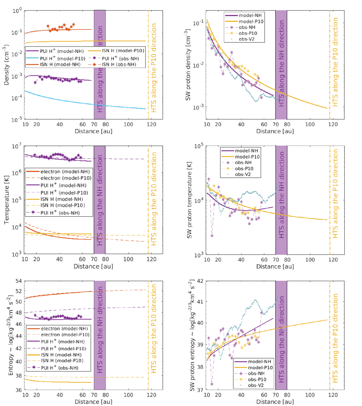
Figure 1. Comparison between the theoretical and observed results as a function of distance in the NH and P10 directions. The top left and right panels illustrate the density; the middle-left and right panels the temperature, and the bottom-left and right panels the entropy for ISN H atoms, H+ PUIs, SW electrons, and the SW protons. The solid and dashed curves denote the theoretical results. The purple/brown and yellow star-dashed star curves denote the observed results measured by NH and P10, respectively. The blue “dots” represent the observed results measured by Voyager 2. The NH and P10 observed values correspond to the averaged values in a bin of width ∼2 au, respectively. The purple-shaded region indicates the crude HTS location ranging between 70 and 80 au along the NH direction. The vertical dashed–dotted line denotes an HTS location at 117.2 au in the downwind direction corresponding to the longitude of 69° and latitude of 3° (B. L. Shrestha et al. 2021).
Download figure:
Standard image High-resolution imageFigure 1 shows the SW parameters describing the density, temperature, and entropy for protons, electrons, H+ PUIs, and ISN H atoms as a function of heliocentric distance. In the NH direction (top left panel), the theoretical results of the ISN H density and the H+ PUI density are comparable with the derived ISN H density and the measured H+ PUI density. Here, we use a different method than P. Swaczyna et al. (2020) to derive the ISN H density (see the Appendix). We found that our results are consistent with those of P. Swaczyna et al. (2020), but are not shown in this manuscript. The theoretical H+ PUI density is consistent with the NH measured H+ PUI density along the NH direction (see also D. J. McComas et al. 2025). The ISN H and H+ PUI density is larger in the NH direction than in the P10 direction as a function of distance. This may be associated with the ISN H atoms entering the heliosphere from its nose direction (see also Figures 5 and 9 in J. M. Sokół et al. 2019a, which are based on time and spatial-dependent modeling of ISN and PUI based on an empirical model of ionization rates). The H+ PUI density falls more rapidly along the P10 trajectory until near the HTS position (i.e., 115 au) in the downwind direction compared to that along the NH trajectory until near the HTS position (i.e., 68 au) in the upwind direction. This result may indicate that the turbulence in the NH direction is stronger than in the P10 direction, as the PUI source of turbulence is proportional to the ISN H density (see Equation (19)). This is also confirmed by the increase in proton temperature in the NH direction with increasing distance in the outer heliosphere compared to that in the P10 direction (middle right panel of Figure 1, see also G. P. Zank et al. 2018b; M. Nakanotani et al. 2020; L. Adhikari et al. 2021).
In the top-right panel of Figure 1, both the theoretical and observed SW proton density show similar radial trends between ∼10 and 58 au in the NH and P10 directions, and the theoretical results in both directions further decrease with increasing distance. The NH measured proton density is similar to the V2 measured proton density from 10 to ∼25 au, and afterward, the NH measured proton density becomes larger. On the other hand, the P10 measured proton density remains larger than that measured by NH and V2 as a function of distance. This may be related with the measurements were made at different moments in time and different directions (D. McComas et al. 2008; J. M. Sokół et al. 2013).
The middle left panel of Figure 1 shows the temperature for electrons, H+ PUIs, and the ISN H atoms. In the NH direction, the theoretical electron temperature decreases gradually with increasing distance until ∼50 au, after which it remains nearly constant until reaching 68 au. In the P10 direction, the theoretical electron temperature decreases monotonically as a function of distance. This difference in electron temperature in the NH and P10 directions may be due to different PUI sources of turbulence (see the right panel of Figure 4) that drive turbulence in the outer heliosphere. The theoretical H+ PUI temperature in the NH direction decreases with increasing distance and captures the overall radial trend of the NH measured H+ PUI temperature (see also P. Mostafavi et al. 2025), in which the observed PUI temperature shows a variability (see also D. J. McComas et al. 2025). The theoretical H+ PUI temperature in the P10 direction becomes slightly larger and decreases more slowly than that in the NH direction. The ISN H temperature in the NH and P10 directions remains approximately constant as a function of distance, being larger in the NH direction.
The theoretical proton temperature is consistent with the observed proton temperature measured by NH and P10 between ∼10 and 58 au (middle-right panel of Figure 1). The P10 measured Ts is larger than the NH measured Ts from 10 to ∼33 au, and then the two temperatures are approximately similar until ∼55 au. The theoretical Ts in the P10 direction is larger than the theoretical Ts in the NH direction within 56 au and then becomes lower than that in the NH direction. The higher proton temperature in the P10 direction compared to the NH direction may result from the effect of including a turbulent shear source in the P10 direction. On the other hand, the V2 measured Ts is similar to the NH measured Ts from 10 to ∼25 au, after which the temperature in the V2 direction increases. The P10 measured Ts is larger than the V2 measured temperature from 15 to 29 au, and the V2 measured Ts becomes larger than the P10 measured Ts after 33 au. The larger proton temperature measured by V2 is that during the years 1995–1999 of the solar minimum, V2 was located outside the sector zone (L. F. Burlaga et al. 2003), within the high-speed streams characterized by high proton temperature.
The bottom-left and right panels of Figure 1 illustrate the entropy  , where a refers to protons, electrons, ISN H atoms, and H+ PUIs) as a function of distance. The theoretical ISN H entropy is approximately constant with increasing distance in the NH and P10 directions. The theoretical H+ PUI entropy in the NH direction is also approximately constant and is similar to the NH measured H+ PUI entropy. However, the theoretical H+ PUI entropy in the P10 direction increases as distance increases. The theoretical and observed electron and proton entropy increases with distance in both directions, where the proton entropy in the NH direction increases more rapidly after 30 au compared to the P10 direction. Similarly, the proton entropy in the V2 direction, beyond 28 au, increases more rapidly in comparison to that in the NH and P10 directions.
The averaged NH measured SW speed is about 329 km s−1 at ∼14 au, which increases gradually to 423 km s−1 at ∼20 au, and then decreases to 356 km s−1 at ∼25.7 au. The speed again increases, followed by a decrease, and then an increase up and until reaching ∼58 au. Here, the SW speed measured near 20 au was during the inclining phase of SC 24, and that near 25 au was during its solar maximum. Similarly, the SW speed observed near 58 au was during the solar maximum of SC 25. However, the theoretical SW speed, being calculated from a steady-state model, decreases gradually as a function of distance and captures the overall radial trend of the SW speed measured by NH. On the other hand, the P10 measured speed is about 430 km s−1 at 11 au, which decreases initially and then increases to about ∼480 km s−1 at ∼35 au. Afterward, the speed decreases and then increases with increasing distance until ∼54 au. In this case, the SW speed measured (i) at about 11 au was during the solar minimum of SC 20, (ii) at about 35 au was near the solar minimum of SC 21, and (iii) at about 54 au was during the solar maximum of SC 22. The theoretical SW speed in the P10 direction decreases slightly from 10 to 115 au, and captures the radial trend of the P10 measured SW speed. While both spacecraft measured different SW speeds during different SC phases, the SW speed was evolving radially. As shown in the left panel of Figure (2), the radial trend of the NH measured speed is decreasing as a function of distance, similar to the theoretical SW speed. This suggests that the gradual variation in the SW speed may be considered as due to radial evolution. The theoretical ISN H speed in the NH and P10 directions is approximately constant with increasing distance. The V2 measured SW speed is about ∼472 km s−1 at 10 au, which decreases to about 383 km s−1 at ∼22 au. The speed then increases gradually to about 530 km s−2 at 51 au and decreases to 380 km s−1 at ∼66 au, which again increases until reaching 75 au.
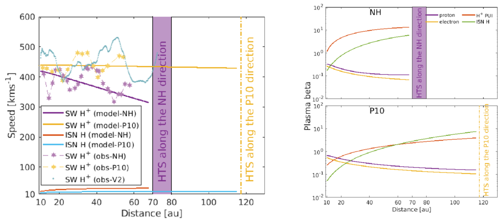
Figure 2. Left panel: SW and ISN H speed as a function of distance in the NH and P10 directions. Right panel: plasma beta corresponding to protons, electrons, H+ PUIs, and ISN H atoms with increasing distance in the NH and P10 directions. The solid and dashed-star-dashed curves denote the theoretical and observed results, respectively.
Download figure:
Standard image High-resolution imageWe plot the theoretical plasma beta for protons, electrons, H+ PUIs, and ISN H atoms as a function of distance (right panel of Figure 2). The proton and electron plasma beta in the NH and P10 directions decrease with increasing distance. The H+ PUI plasma beta in the NH and P10 directions increases rapidly between 10 and ∼30 au and then more gradually as a function of distance. Similarly, the ISN H plasma beta in both directions increases with increasing distance, simply because the ISN H temperature remains constant and the magnetic field decreases with increasing heliocentric distance.
We plot the relationship between the theoretical proton temperature and the theoretical SW speed, and the theoretical electron temperature and the theoretical SW speed in the NH and P10 directions in Figure 3. In the NH direction, the theoretical Ts and the theoretical SW speed are positively correlated between 10 and ∼ 35 au, and beyond 35 au, they are anticorrelated. Such an anticorrelation between Ts and SW speed has not been reported before in the literature, which may not be clear in the V2 data because of the solar cycle dependence of the SW speed (see the left panel of Figure 2). For example, J. S. Halekas et al. (2020), D. Telloni et al. (2022), and S. P. Gautam et al. (2024) reported that the Ts and the SW speed are correlated in the inner heliosphere and at 1 au. On the other hand, the electron temperature Te and the SW speed in the NH direction show a positive correlation between 10 and ∼45 au, and beyond 50 au, there is a weak correlation. In the P10 direction, the Ts and Te do not exhibit any clear correlation with the SW speed between 10 and ∼50 au, and then they show a positive correlation.
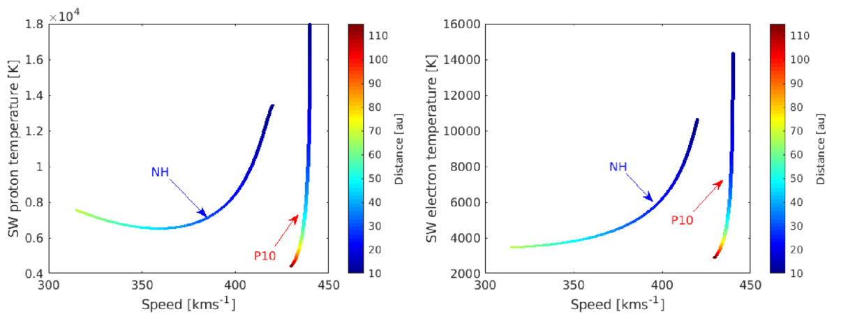
Figure 3. Relationship between the theoretical proton temperature and the theoretical SW speed (left panel) and the theoretical electron temperature and the theoretical SW speed (right panel) in the NH and P10 directions. The color bar denotes the radial distance.
Download figure:
Standard image High-resolution imageThe left panel of Figure 4 shows a larger turbulent heating rate in the P10 direction than in the NH direction between 10 au and ∼55 au, after which the heating rate in the NH direction becomes larger. The right panel shows that the PUI source of turbulence in the NH direction increases rapidly between 10 and 30 au, then increases gradually until 50 au, and then shows a slight decrease with increasing distance. In the P10 direction, the PUI source of turbulence increases rapidly between 10 and 40 au, and then it shows a gradual increase with increasing distance. The PUI source in the NH direction is ∼4.6–5.7 times that in the P10 direction.
The top-left panel of Figure 5 shows that the normalized PUI source of turbulence is positively correlated with the normalized theoretical ISN H density between 10 and ∼50 au, and between 10 and ∼110 au in the NH and P10 directions, respectively. In the outer heliosphere along the NH direction, the PUI source and the theoretical ISN H density increase by factors of ∼1.45 and ∼1.58 compared to those at 10 au. In the P10 direction, the PUI source and the theoretical ISN H density increase by factors of ∼1.25 and ∼1.25 compared to those at 10 au.
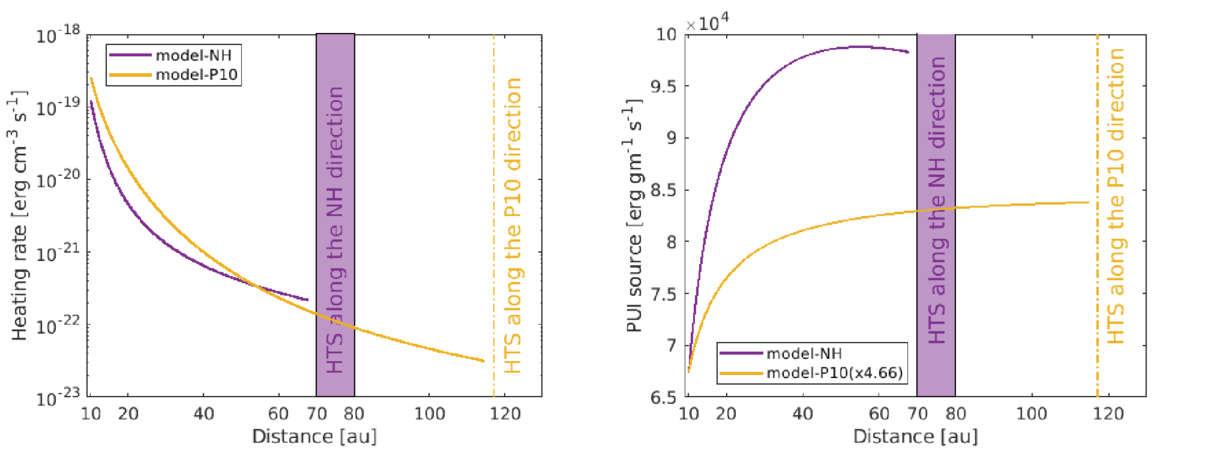
Figure 4. Theoretical turbulent heating rate (left panel) and the theoretical PUI source of turbulence (right panel) in the NH and P10 directions as a function of distance. The PUI source of turbulence in the P10 direction is multiplied by 4.66 for better visualization.
Download figure:
Standard image High-resolution image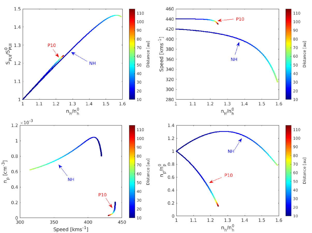
Figure 5. Relationship between the normalized PUI source of turbulence and the normalized theoretical ISN H density (top left), the theoretical SW speed and the normalized theoretical ISN H density (top right), the theoretical H+ PUI density and the theoretical SW speed (bottom left), and the theoretical H+ PUI density and the normalized theoretical ISN H density in the NH and P10 directions.
Download figure:
Standard image High-resolution imageThe top-right panel of Figure 5 illustrates the relationship between the theoretical SW speed and the normalized theoretical ISN H density. In the NH direction, the speed decreases gradually with increasing ISN H density until nh/nh0 ∼ 1.4 and then decreases rapidly. In the P10 direction, the speed remains approximately constant until nh/nh0 ∼ 1.2 and then decreases rapidly. The theoretical H+ PUI density and the theoretical SW speed in the NH direction initially show a negative correlation between 10 and ∼20 au, and then a positive correlation, while in the P10 direction, they show a positive correlation beyond ∼55 au (bottom-left panel). Also, the normalized theoretical H+ PUI and ISN H density shows a positive correlation in the NH direction from 10 to ∼20 au, and then a negative correlation. However, they show a negative correlation throughout the P10 direction (bottom-right panel).
The top and middle left panels of Figure 6 depict the outward and inward Elsässer energies as functions of distance. Both the theoretical outward and inward Elsässer energies in the NH direction decrease until ∼25 au and then increase gradually with increasing distance until 68 au, while those in the P10 direction decrease monotonically, although more slowly in the outer heliosphere. The difference in the Elsässer energies in the NH and P10 directions is due to different PUI sources of turbulence (see the right panel of Figure 4), in which the PUI source of turbulence in the NH direction is larger. Also, the theoretical outward and inward Elsässer energies in the NH and P10 directions are lower than those measured by V2. Although there is no direct comparison since V2 is located at different latitudes than NH and P10, these results indicate that the SW is more turbulent in the V2 direction than in the NH and P10 directions. The top and middle right panels show the correlation length corresponding to outward and inward Elsässer energies with increasing heliocentric distance. The theoretical correlation lengths λ+ and λ− in the P10 direction increase gradually with increasing distance, while those in the upwind direction increase more rapidly. The derived λ+ and λ− from the V2 measurements are lower than the theoretical results along the NH and P10 directions.
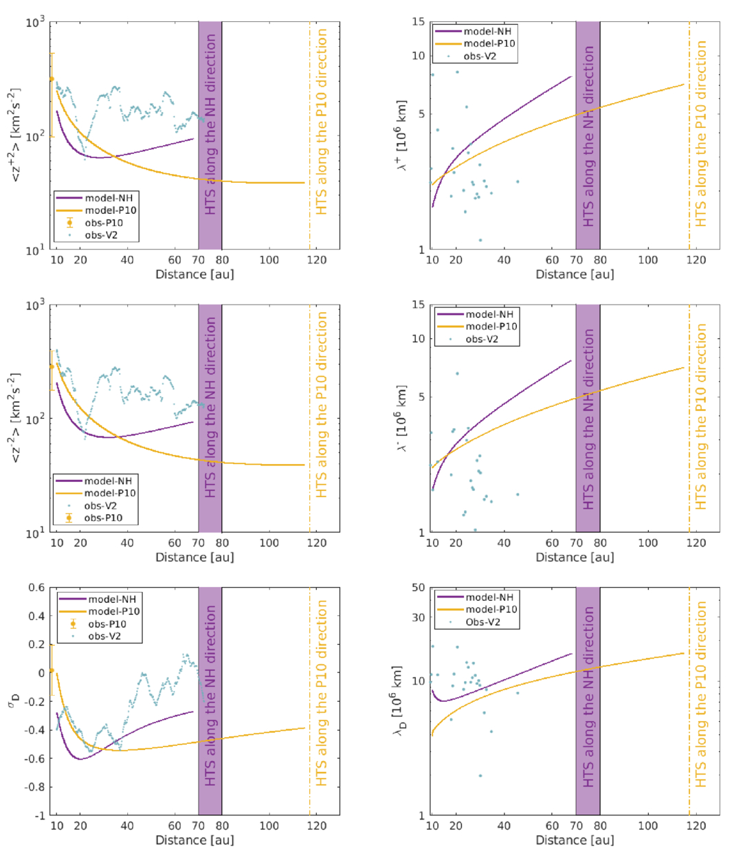
Figure 6. Turbulence energy and the corresponding correlation length as a function of distance in the NH, P10, and V2 directions. The top left and right panels denote the outward Elsässer energy and the corresponding correlation length. The middle left and right panels denote the inward Elsässer energy and the corresponding correlation length. The bottom-left and right panels denote the normalized residual energy and the correlation length of the residual energy. The solid curves denote the theoretical results. The scatter plots denote the observed results. The V2-derived results are taken from L. Adhikari et al. (2023).
Download figure:
Standard image High-resolution imageThe bottom-left and right panels of Figure 6 show the normalized residual energy σD and the correlation length of the residual energy as a function of distance. The σD is more negative along the NH direction than along the P10 direction within 30 au, indicating that the fluctuations are more magnetically dominated along the NH direction. However, afterward, it reverses, in which σD increases more rapidly in the NH direction than in the P10 direction. In the outer heliosphere, the derived σD along the V2 trajectory increases toward zero with increasing distance, indicating that the fluctuations become less magnetically dominated along the V2 direction as distance increases.
The top left and right panels of Figure 7 show the theoretical fluctuating magnetic energy and the corresponding correlation length along the NH and P10 directions, and the derived turbulent magnetic energy and the correlation length along the V2 direction. The theoretical 〈B2〉 in the NH and P10 directions, and the derived 〈B2〉 along the V2 direction, fall gradually with increasing distance. The decreasing rate of 〈B2〉 along the NH direction is slower than along the P10 direction in the outer heliosphere. Similarly, the bottom-left and right panels show the fluctuating kinetic energy and the corresponding correlation length along the NH, P10, and V2 directions as a function of distance.
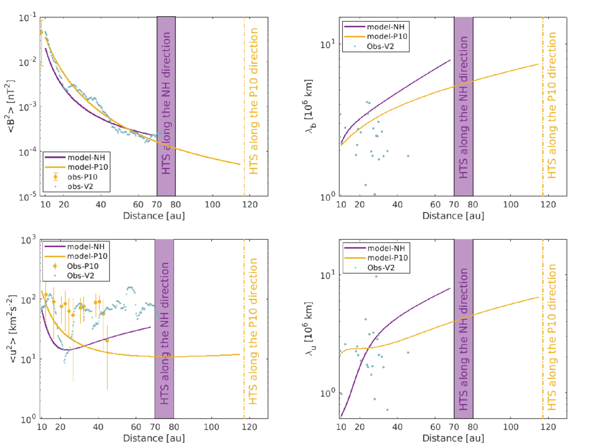
Figure 7. Top-left and right panels: fluctuating magnetic energy and the corresponding correlation length in the NH, P10, and V2 directions. Bottom-left and right panels: fluctuating kinetic energy and the corresponding correlation length in the NH, P10, and V2 directions. The solid curves denote the theoretical results. The scatter plots denote the observed results. The V2-derived results are taken from L. Adhikari et al. (2023).
Download figure:
Standard image High-resolution imageFigure 8 shows that between 10 and ∼20 au, the theoretical cross-helicity σc in the NH and P10 directions is approximately similar, and then the σc in the NH direction increases more rapidly than P10 direction. The σc is close to zero along the NH direction in the outer heliosphere, indicating that turbulence is balanced, i.e., the outward and inward Elsässer energy fluxes are equal, whereas σc ≠ 0 is along the P10 direction in the outer heliosphere. Similarly, the derived σc from the V2 measurements is nearly zero between 20 and 80 au, also suggesting that the inward energy flux is nearly equal to the outward energy flux.
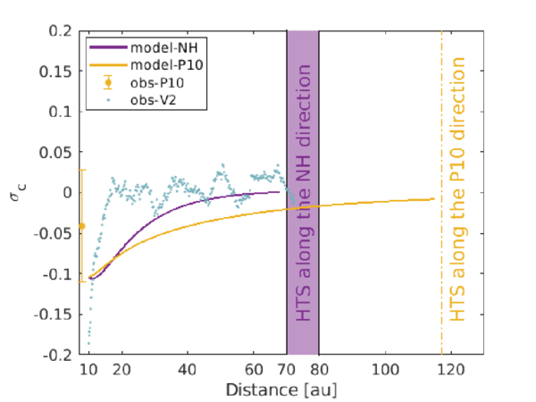
Figure 8. Normalized cross-helicity as a function of distance in the NH, P10, and V2 directions. The solid curves denote the theoretical results. The scatter plots denote the observed results. The V2-derived results are taken from L. Adhikari et al. (2023).
Download figure:
Standard image High-resolution imageThe top left panel of Figure 9 illustrates the relationship between the PUI source of turbulence and the theoretical total turbulent energy ET( = (〈z+2〉 + 〈z−2〉)/2) as a function of distance. In the P10 direction, the PUI source of turbulence and the theoretical ET exhibit a negative correlation with increasing distance. In the NH direction, the PUI source of turbulence is negatively correlated with the theoretical ET between 10 and ∼25 au, and then they do not exhibit a clear correlation. Similarly, the theoretical ET shows a positive correlation with the theoretical Ts and Te between 10 and ∼90 au in the P10 direction, although both decrease with increasing distance. In the NH direction, ET and Ts are positively correlated first in the distance between 10 and ∼30 au, and second in the distance between 40 and 68 au, wherein the prior distances both decrease, and in the latter distances both increase. Similarly, ET and Te show a positive correlation from 10 to ∼35 au, followed by a slight negative correlation, and no clear correlation.
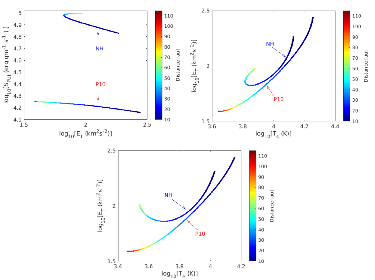
Figure 9. Relationship between the PUI source of turbulence and the theoretical total turbulent energy (top left panel), the theoretical total turbulent energy and the theoretical proton temperature (top-right panel), and the theoretical total turbulent energy and the theoretical electron temperature (bottom panel) in the NH and P10 directions. The color bar denotes the radial distance.
Download figure:
Standard image High-resolution image4. Density Turbulence and Angular Broadening of Radio Sources
The scattering of radiation by density turbulence between a source and an observer results in changes in the apparent direction and angular size of the source, scintillation of the intensity, and dispersion of the signal (L. C. Lee & J. R. Jokipii 1975; B. J. Rickett 1977). These phenomena arise due to density irregularities that disperse, reflect, or alter the phase of the radiation along the propagation path. In particular, angular broadening is mainly attributed to phase changes caused by refraction and diffraction along the path, and less typically by reflections. These processes are often grouped as “scattering” by density turbulence.
The parabolic wave equation theory predicts the angular broadening of the radio waves due to scattering by density perturbations. It considers locally planar EM radiation with a wavenumber k and a scalar electric field ϕ in a plane perpendicular to the propagation direction z of the EM radiation. The statistical properties of the scalar field ϕ are characterized by an infinite series of moments or correlation functions of the scalar field. So,

where the angle brackets denote an ensemble average, s denotes a position vector in a plane perpendicular to the propagation direction, and k1 and k0 denote the wavenumbers. The correlation function Γ1,1(z, k0, k0, s) using the Markov approximation can be written in the form (see L. C. Lee & J. R. Jokipii 1975; I. H. Cairns 1998, for details),

where re is the electron radius, A(z, s) is the transverse correlation function, and λfs( = c/f, c is the speed of light, and f the frequency of the radiation) is the free space wavelength. The path integral of Equation (24) is given by
where fp0 is the plasma frequency. The 2D Fourier transform A(z, s) can be written in the form (I. H. Cairns 1998),

where k denotes the wavevector perpendicular to the propagation direction, and P3N(z, 0, k) the 3D power spectral density (PSD). Assuming that P3N(z, 0, k) exhibits a Kolmogorov-type of power law, together with an assumed inner scale, we have (see L. C. Lee & J. R. Jokipii 1975; B. J. Rickett 1977; S. Tasnim et al. 2022),

where  is the amplitude of density fluctuations, α = 11/3, ki = 2π/li, li( = 2πrg = 2πmpvth/(qsB)) is the inner scale,
  is the proton thermal speed, qs is the charge, and rs is the proton gyroradius.
The integration of Equation (26) using Equation (27) yields

where 1F1 is a hypergeometric function. We use  , for x ≪ 1, in Equation (28), yielding

For Gaussian density turbulence, the transverse scale of Γ1,1 is simply that value of s for which (see L. C. Lee & J. R. Jokipii 1975; B. J. Rickett 1977)

from Equation (25). Using Equation (29) in Equation (30) yields
We assume that the characteristic length scale sc and the scattering angle θsc follow the relationship (L. C. Lee & J. R. Jokipii 1975)

Using kfs = 2π/λfs and Equations (31) in (32) yields the scattering angle in the form,
In Equation (33), the path integral along z from the source z = 0 to the observer z = zobs can be reformulated as an integral over the radial path integral from the radio wave source r = rso to the observer r = rob as follows (see also S. Tasnim et al. 2022):
To calculate the scattering angle, Equation (34) requires the amplitude of the density turbulence  and the frequency fp0(r). We use the radial dependent frequency fp0(r) as in I. H. Cairns (1995).
  is obtained by equating the PSDs of the density turbulence in the energy-containing range and the inertial range at the wavenumber corresponding to the injection scale (see L. Adhikari et al. 2017b; S. Tasnim et al. 2022). The expression for
  is given by

where 〈ρ2〉 is the variance of density fluctuations, and kinj ( = 2π/(U × 28 days)) the injection wavenumber. The 〈ρ2〉 is obtained by solving the following transport equation (G. P. Zank et al. 2017; L. Adhikari et al. 2023):
where α2 is the von Kármán–Taylor constant, η1 is the strength of the turbulent shear source, η2 is the fraction of PUI source of turbulence allocated to drive density fluctuations,  is the variance of density fluctuations at r = r0. Here, the density fluctuations sit passively on the velocity fluctuations and are advected by turbulent velocity fluctuations. The first, second, and third terms on the rhs of Equation (36) denote the decay term, turbulent shear source, and the PUI source of turbulence. Again, we note that the turbulence shear source is not included in the upwind direction. In the absence of rhs terms and (i) for a constant SW speed, the 〈ρ2〉 falls as r−4; (ii) for a decelerating SW speed, the 〈ρ2〉 falls slower than r−4, and (iii) for an accelerating SW speed, the 〈ρ2〉 falls faster than r−4. However, the presence of a decay term leads to a faster decrease of 〈ρ2〉 than r−4, even for a decelerating SW flow (L. Adhikari et al. 2017a, 2023; G. P. Zank et al. 2017, 2018b).
5. Evolution of Density Turbulence and Radio Wave Scattering
The variance of density fluctuations decreases with increasing distance along the NH, P10, and V2 trajectories (left panel of Figure 10). Although the decreasing rate of density fluctuations varies depending on the heliocentric distances, the density fluctuations decrease more rapidly than r−4. This faster decrease may be related to a fast interaction time between the eddy of density fluctuations and the characteristic speed of velocity fluctuations, resulting in a strong decay term (indicating strong turbulence). Specifically, the theoretical and derived 〈ρ2〉 are consistent along the NH direction between 10 and ∼58 au, and along the P10 direction between 10 and ∼54 au. Thereafter, the theoretical 〈ρ2〉 decreases further with increasing distance in both directions, although more slowly at large distances. The derived 〈ρ2〉 from the V2 measurements is lower and decreases faster than that along the NH and P10 directions. The right panel shows the amplitude of density fluctuations  in the NH and P10 directions with increasing distance.
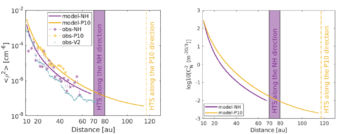
Figure 10. Variance of density fluctuations (left panel) and the amplitude of density fluctuations (right panel) in the NH, P10, and V2 directions as a function of distance. The solid curves denote the theoretical results and the scatter plot the derived results. The V2-derived results are taken from L. Adhikari et al. (2023).
Download figure:
Standard image High-resolution imageThe most likely origin of the radio signals observed by Voyagers is mode conversion from electrostatic waves at or beyond the heliopause, triggered by large shocks associated with global merged interaction regions in the SW that propagate through the inner heliosphere and into the very local ISM (D. A. Gurnett et al. 1993). However, a limitation of this work is the assumption that the radio sources are located at 68 au and 115 au in the NH and P10 directions, respectively, which is within the HTS. In a similar study, S. Tasnim et al. (2022) assumed the source of radio waves to be at 118 au, i.e., beyond the HTS, along the V2 trajectory, and calculated the scattering angle in the higher latitudes as a function of distance. Figure 11 illustrates the scattering angle θsc in the NH and P10 directions as a function of distance, showing that they exhibit different radial profiles along these directions. These results show that having a source of radio waves at larger distances reduces the scattering angle. In the figure, the red square symbol denotes the measured θsc by Voyagers 1 and 2 (D. A. Gurnett et al. 1993; I. H. Cairns 1998), which we include as a reference, and not for comparison with the theoretical results.
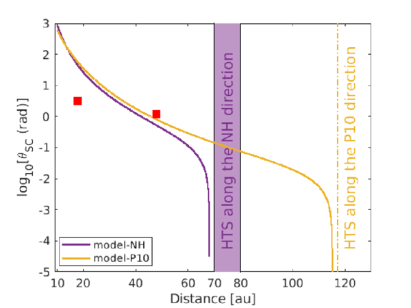
Figure 11. Scattering angle of radio waves θsc in the NH and P10 directions as a function of distance. The solid curves denote the theoretical results. The red square symbols denote the observed results from V2 at 18 au (W. S. Kurth 1988) and V1 at 48 au (D. A. Gurnett et al. 1993).
Download figure:
Standard image High-resolution image6. CR Diffusion Tensor throughout the Heliosphere
An understanding of magnetic turbulence is required to calculate the parallel, perpendicular, and drift components of the CR diffusion tensor (G. P. Zank et al. 1998; V. Florinski et al. 2003; N. E. Engelbrecht & R. A. Burger 2013a, 2013b; L. L. Zhao et al. 2017; L.-L. Zhao et al. 2018; L. Adhikari et al. 2021). Quasi-linear theory (QLT) is widely used to describe particle transport in a magnetized turbulent plasma. The basic principle of QLT assumes a weak perturbation of the charged particle gyro-orbits by EM fluctuations. By including parallel scattering and dynamical turbulence effects, W. H. Matthaeus et al. (2003) proposed a nonlinear guiding center (NLGC; see also G. P. Zank et al. 2004; A. Shalchi et al. 2004a; A. Shalchi 2010, 2013, 2014) theory to describe the perpendicular diffusion of charged particles. Similarly, A. Shalchi et al. (2004b) introduced a weakly nonlinear theory (WNLT) for the parallel and perpendicular diffusion of CRs. In WNLT theory, the nonlinear effect produces a resonance broadening that allows charged particles to scatter through 90° (A. Shalchi et al. 2004b), yielding a nonzero pitch-angle Fokker–Planck coefficient at 90°, and a reasonable parallel diffusion length (A. Shalchi 2005, 2009). Here, we use a simple QLT description (G. P. Zank et al. 1998) and the NLGC theory (W. H. Matthaeus et al. 2003) to calculate the parallel and perpendicular diffusion of energetic charged particles, respectively.
The 2D turbulence power at the outer scale has an important impact on the perpendicular diffusion coefficients of charged particles (N. E. Engelbrecht & R. A. Burger 2015; N. E. Engelbrecht 2019a, 2019b), including galactic cosmic-ray (GCR) proton and electron intensities. Using the observed size of magnetic islands (M. L. Cartwright & M. B. Moldwin 2010), and the estimated outer scales (N. E. Engelbrecht & R. A. Burger 2013b; L. Adhikari et al. 2017b), N. E. Engelbrecht (2019a) found that the GCR electron differential intensities above the kinetic energy of 0.1 GeV are closer to the observed electron differential intensities. Similarly, N. E. Engelbrecht (2019b) introduced a new method for calculating perpendicular diffusion coefficients based on the random ballistic decorrelation interpretation of the NLGC theory proposed by D. Ruffolo et al. (2012). Their results show that the strength and anisotropy of solar energetic particles are highly sensitive to the pitch-angle dependence of the perpendicular diffusion coefficient.
Turbulence responsible for scattering the charged particles (G. P. Zank et al. 1998; L. L. Zhao et al. 2017; L.-L. Zhao et al. 2018; A. Shalchi et al. 2006; A. Shalchi 2018, 2020) in the SW with a plasma beta β ∼ 1 can be described as a superposition of a dominant 2D component and a minority slab component (G. P. Zank et al. 2017, 2020). Here, we first calculate the 〈b2〉 and λb from the 3D NI MHD turbulence transport model equations (see Section 2.3). Then, we determine the 2D  and slab
  turbulence energy according to
  and
and  (see G. P. Zank et al. 2020), and the corresponding correlation lengths by
  and
and  .
.
6.1. CR Diffusion Tensor
The CR diffusion tensor can be written as

where Bi, Bj, and Bk denote the three components of the magnetic field, δij the Kronecker delta tensor, and ijk the Levi–Civita tensor. The parameter κ∣∣ denotes the diffusion parallel to the magnetic field, κ⊥ denotes the diffusion perpendicular to the magnetic field, and κA accounts for the particle drift due to large-scale curvature and gradients in the interplanetary magnetic field.
The radial diffusion coefficient is given by

The winding angle ψ between the magnetic field and the radial direction is written as

where θ is the colatitude with respect to the solar axis rotation. We use θ = 90°. The diffusion tensor in terms of the length scale is given by (G. P. Zank et al. 1998; L. L. Zhao et al. 2017; L.-L. Zhao et al. 2018)

where v is the particle speed.
6.2. CR Parallel Mfp
J. W. Bieber et al. (1994) obtained the mfp for electrons and protons consistent with the Palmer consensus (I. D. Palmer 1982) by considering turbulence as a superposition of a dominant 2D component and a minority slab component. However, when considering only a pure slab model, J. R. Jokipii (1966) found that the mfp for CRs exceeds the Palmer consensus. The parallel mfp based on the standard QLT and assuming magnetostatic turbulence is given by (G. P. Zank et al. 1998),
where
The parameter P( ≡ pc/Ze, where p is the momentum, c the speed of light, and Ze the particle charge) is the particle rigidity, B the magnetic field strength, RL( = P/Bc) the particle Larmor radius, and  (
( ) the variance of the x component of the slab fluctuations. Equation (41) closely approximates the exact Fokker–Planck form, but may lose accuracy at very small rigidities in which the dynamical MHD turbulence plays a significant role (J. W. Bieber et al. 1994; G. P. Zank et al. 1998). The fractional term inside the squared brackets becomes particularly important when the Larmor radius is equal to or larger than the slab correlation length λslab. In such conditions, the ions resonate with the turbulent MHD fluctuations in the energy-containing range, but not with the fluctuations in the inertial range.
6.3. CR Perpendicular Mfp
The perpendicular mfp Λ⊥ can be calculated by the hard sphere scattering approach (W. I. Axford 1965; L. J. Gleeson & W. I. Axford 1967) and the Green–Kubo–Taylor formula (J. W. Bieber & W. H. Matthaeus 1997). Here, we use the NLGC theory (W. H. Matthaeus et al. 2003), which assumes that the perpendicular diffusion is controlled by the velocity of gyrocenters along the field line. The NLGC theory, therefore, incorporates both the random walk of the magnetic field line and the parallel scattering of CRs. The perpendicular mfp is given by (G. P. Zank et al. 2004),
and
where a2 is the coefficient corresponding to the gyrocenter velocity, and is numerically found to be ∼1/3, and  is a constant related to the spectral index 2ν, where Γ(ν) is the gamma function.
7. Evolution of the CR Mfp
Figure 12 shows the theoretical perpendicular, parallel, and radial mfps for a proton with rigidity 445 MV (or equivalent to a 100 MeV proton) in the NH and P10 directions. The parallel mfp in the NH direction increases rapidly between 10 and 40 au, and then increases more gradually up to 68 au. Similarly, the parallel mfp along the P10 direction increases rapidly between 10 and 40 au, and then increases monotonically until 115 au. The perpendicular mfp in the NH direction increases slightly faster than that in the P10 direction with increasing heliocentric distance. The radial mfp in the NH direction decreases with increasing distance between 12 and 68 au, while that in the P10 direction remains approximately constant between 12 and 115 au.
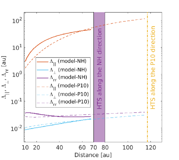
Figure 12. Perpendicular, parallel, and radial mfps in the NH and P10 directions as a function of distance. The solid curves denote the NH direction, and the dashed curves the P10 direction.
Download figure:
Standard image High-resolution image8. Discussion and Conclusions
We studied the impact of physical processes on the radial evolution of the PUI-mediated plasma in the upwind and downwind directions along the NH and P10 directions, respectively, where H+ PUIs play a crucial role in governing the SW dynamics. For this, we solved numerically the coupled four-fluid SW model equations describing protons, electrons, H+ PUIs, and ISN H atoms, and a high plasma beta regime form of the NI MHD turbulence transport equations. We integrated the continuity, momentum, and pressure equations for ISN H atoms to determine the ISN H density as a function of distance (see Y. C. Whang 1996; H. J. Fahr et al. 2000; A. V. Usmanov et al. 2016; M. Opher et al. 2020), which was used to calculate the PUI source of turbulence (G. P. Zank et al. 1996) that drives turbulence in the outer heliosphere. The size of the ionization cavity for hydrogen atoms in the downwind direction is ∼22.51 au and in the upwind direction is ∼4.2 au (D. Rucinski & M. Bzowski 1995), which may vary with the solar activity and the conditions of the SW (J. M. Sokół et al. 2019a). This indicates that the H+ PUIs impact the SW in the upwind direction at a closer distance from the Sun than in the downwind direction. In the NH direction, we solved the turbulence-driven SW model equations from 10 to 68 au before the HTS located in the upwind direction. Similarly, in the P10 direction, we solved the model equations from 10 to 115 au before the HTS located in the downwind direction.
The Voyager missions made a significant discovery by detecting low-frequency radio wave emissions in the distant heliosphere (W. S. Kurth 1988; D. A. Gurnett et al. 1993). The irregularities present in the SW plasma density may scatter these radio waves, identified by the radio wave scattering angle. Although we do not study the scattering angle of radio waves along the Voyagers' trajectories in this work, we derived the equation for the scattering angle of the broadening of radio waves to calculate the scattering angle of such radio waves in the NH and P10 directions. Note that NH is not equipped with a magnetometer to measure the magnetic field, and the magnetic field data is unavailable in the P10 data sets beyond 10 au, leaving the observational analysis of low-frequency MHD turbulence unknown. In this study, by comparing the theoretical results with SW and H+ PUI data measured by NH, and the SW data measured by P10, we predicted the low-frequency MHD turbulence intensities and the corresponding correlation lengths along the NH and P10 directions. Also, using the theoretical results of the fluctuating magnetic energy and the correlation length of the magnetic field fluctuations, we estimated the CRs perpendicular, parallel, and radial mfps in the NH and P10 directions. In Table 3, we show the values of the SW, H+ PUI, and ISN H parameters, turbulence quantities, and CR mfps in the NH direction at 68 au and in the P10 direction at 115 au.
Table 3. Predicted Model Values of the Plasma and Turbulence Quantities Before the HTS at 68 au in the NH (Upwind) Direction and at 115 au in the P10 (Downwind) Direction
| Quantities | NH Direction | P10 Direction | Quantities | NH Direction | P10 Direction | |
|---|---|---|---|---|---|---|
| (68 au) | (115 au) | (68 au) | (115 au) | |||
| U [km s−1] | 315 | 429.7 | np [cm−3] | 6.23 × 10⁻⁴ | 3.14 × 10⁻⁵ | |
| SW | ns [cm−3] | 1.86 × 10⁻³ | 9.25 × 10⁻⁴ | Tp [K] | 2.69 × 10⁶ | 3.22 × 10⁶ |
| + | Ts [K] | 7.55 × 10³ | 4.39 × 10³ | UH [km s−1] | 31.0 | 19.53 |
| H+ PUI | Te [K] | 3.46 × 10³ | 2.88 × 10³ | nH [cm−3] | 0.135 | 3.98 × 10⁻² |
| + | Ss [ (kg−2/3 km4 s−2 )] (kg−2/3 km4 s−2 )] | 40.22 | 40.14 | TH [K] | 5.57 × 10³ | 4.83 × 10³ |
| ISN H | Se [ (kg−2/3 km4 s−2 )] (kg−2/3 km4 s−2 )] | 51.96 | 52.25 | ⋯ | ⋯ | ⋯ |
SPUI [ (kg−2/3 km4 s−2 )] (kg−2/3 km4 s−2 )] | 46.82 | 48.99 | ⋯ | ⋯ | ⋯ | |
SH [ (kg−2/3 km4 s−2 )] (kg−2/3 km4 s−2 )] | 37.06 | 37.73 | ⋯ | ⋯ | ⋯ | |
| Plasma beta | βs | 0.11 | 0.15 | βPUI | 13.58 | 3.92 |
| βe | 0.068 | 0.107 | βH | 6.1 | 7.48 | |
 [km2 s−2] [km2 s−2] | 94.24 | 38.72 | λ+ [106 km] | 7.84 | 7.13 | |
 [km2 s−2] [km2 s−2] | 94.01 | 39.30 | λ− [106 km] | 7.74 | 7.11 | |
| ED [km2 s−2] | −25.37 | −15.03 | λD [106 km] | 16.10 | 16.22 | |
| Turbulence | 〈B2〉 [nT2] | 2.33 × 10⁻⁴ | 5.25 × 10⁻⁵ | λb [106 km] | 7.85 | 7.39 |
| 〈u2〉 [km2 s−2] | 34.38 | 12.00 | λu [106 km] | 7.69 | 6.49 | |
| 〈ρ2〉 [cm−6] | 1.75 × 10⁻⁷ | 3.65 × 10⁻⁸ | σc | 1.24 × 10⁻³ | −7.43 × 10⁻³ | |
 [m−20/3] [m−20/3] | 1.00 × 10⁻² | 2.1 × 10⁻³ | σD | −0.269 | −0.385 | |
 [erg gm−1 s−1] [erg gm−1 s−1] | 9.83 × 10⁴ | 1.79 × 10⁴ | ⋯ | ⋯ | ⋯ | |
| CR | Λ⊥ [au] | 0.022 | 0.03 | Λ∣∣ [au] | 46.16 | 115.06 |
| Λrr [au] | 0.028 | 0.039 | ⋯ | ⋯ | ⋯ | |
Download table as: ASCIITypeset image
We summarize our basic conclusions as follows.
- 1.We derived the ISN H density using the H+ PUI density and the SW speed measured at different heliocentric distances by the NH spacecraft. Our method differs from P. Swaczyna et al. (2020), but the results are consistent. The derived ISN H density is similar to the theoretical ISN H density as a function of distance. The theoretical ISN H density in the NH direction is larger than that in the P10 direction. Similarly, the theoretical and observed H+ PUI density in the NH direction is consistent and is larger than that in the P10 direction. The proton density in the P10 direction is larger than that in the NH direction. The proton density in the V2 direction remains lower than the two other measurements in the outer heliosphere.
- 2.The PUI source of turbulence is proportional to the ISN H density. The PUI source of turbulence in the NH direction is about 4.6–5.7 times larger than the PUI source of turbulence in the P10 direction.
- 3.The ISN H temperature is approximately constant in the NH and P10 directions, being larger in the NH direction. The theoretical H+ PUI temperature in the NH and P10 directions decreases with increasing distance, and the decrease is slower in the P10 direction. The electron temperature in the NH direction decreases with increasing distance and flattens in the outer heliosphere, due to the H+ PUIs generated turbulence. In the P10 direction, since the PUI-generated turbulence is not strong, the electron temperature decreases gradually with distance. Similarly, the proton temperature in the P10 direction decreases monotonically, while that in the NH direction increases after 40 au. The V2 measured proton temperature remains larger than that measured by NH and P10 in the outer heliosphere.
- 4.The theoretical ISN H speed increases slightly with increasing distance in the NH and P10 directions. On the other hand, the theoretical SW speed in the NH direction decreases gradually from 420 and 293 km s−1 with increasing distance. In the P10 direction, the SW speed decreases slightly from 440 and ∼416 km s−1 as a function of distance.
- 5.The proton temperature and SW speed in the NH direction show a positive correlation between 10 and ∼35 au, while they are anticorrelated between ∼50 and 68 au. Whereas, they do not show any correlations between ∼35 and ∼50 au. Such an anticorrelation between proton temperature and SW speed has not been reported before in the literature. For example, D. Telloni et al. (2022), J. S. Halekas et al. (2020), and S. P. Gautam et al. (2024) reported the correlation between the SW proton temperature and the SW speed in the inner heliosphere and at 1 au. In the P10 direction, the proton temperature and SW speed show a positive correlation only beyond ∼50 au, and within 50 au, there is no clear correlation. Additionally, the electron temperature and SW speed show a positive correlation in the NH direction between 10 and ∼50 au, and in the P10 direction after ∼80 au.
- 6.The outward and inward Elsässer energies in the NH direction increase with increasing distance in the outer heliosphere, while those in the P10 direction decrease gradually as distance increases. The intensity of Elsässer energies measured by V2 is larger compared to that along the NH and P10 trajectories.
- 7.The variance of the density fluctuations falls differently along the P10, NH, and V2 trajectories. In the outer heliosphere, the density fluctuations in the P10 direction exhibit the largest value, while those in the V2 direction show the lowest value.
- 8.As in S. Tasnim et al. (2022), we derived the equation for the scattering angle of radio waves using an isotropic and Gaussian density turbulence spectrum in the inertial range (L. C. Lee & J. R. Jokipii 1975; B. J. Rickett 1977) that includes the inner scale. However, density turbulence can become anisotropic in the dissipation range (E. P. Kontar et al. 2023), and in such a case, the radio wave scattering may exhibit anisotropic characteristics (X. Chen et al. 2023). This is beyond the scope of this paper and will be included in future work.
- 9.The amplitude of density fluctuations
 and the scattering angle θsc are predicted along the NH and P10 directions, including the effect of the inner scale. One of the effects of the inner scale is that it significantly decreases the scattering angle (e.g., S. Tasnim et al. 2022). The and θsc decrease as a function of distance in both directions.
 - 10.Instead of a WNLT (A. Shalchi et al. 2004b), we used a simple quasi-linear theory (G. P. Zank et al. 1998) and the NLGC theory (W. H. Matthaeus et al. 2003) to calculate the CR parallel and perpendicular mfps throughout the heliosphere. Initially, the parallel mfp in the NH direction increases rapidly, and then more gradually with increasing distance, while that in the P10 direction increases monotonically as a function of distance. The perpendicular mfp in the NH direction increases slightly faster than that in the P10 direction. Additionally, the radial mfp decreases monotonically along the NH direction, while that in the P10 direction is approximately constant.


This paper extends our previous work (G. P. Zank et al. 2018b; L. Adhikari et al. 2023) by including a separate fluid component for ISN H. We studied comparatively the collective behavior of SW protons and electrons, H+ PUIs, ISN H atoms, low-frequency MHD turbulence, radio wave scattering, and CR mfps along the NH and P10 directions before the corresponding HTS locations. We also presented the V2 measured results as a reference, but not for direct comparisons with the theoretical and observed results corresponding to NH and P10 directions. As NH is approaching the HTS, the results presented in the study are important for understanding the physical processes in the PUI-mediated plasma in the outer heliosphere.
Acknowledgments
We acknowledge the partial support of a NASA Heliospheric Shield award 80NSSC22M0164, BU SAP No. 50210276, a Parker Solar Probe contract SV4-84017, an NSF EPSCoR RII-Track-1 cooperative agreement OIA-2148653, and NASA awards 80NSSC20K1783, 80NSSC21K1319, and 80NSSC25K7672. D.J.M. was supported by the IMAP mission, as part of NASA’s Solar Terrestrial Probes (STP) mission line (80GSFC19C0027). The NH work was supported by NASA NH funding through contract NAS5-97271/Task order 30.
Appendix: Calculation of ISN H density
Using the SW speed and the H+ PUI density measured by NH, we derive the column density NH(r) as a function of distance using the following equation (P. Swaczyna et al. 2020),

where β0 is the ionization rate at r0. Figure 13 shows the Carrington rotation-averaged NH values as a function of distance (black dots). We further smooth the column density by using moving intervals of 100 data points, which is shown by blue triangles. We use these blue-derived results to calculate the ISN H density. For this, we use a moving window of 2 au width, in which we fit the scatter plots of NH(r) versus r using the function y = 10axb, where y represents column density, x represents distance, and a and b are determined by fitting. Using the fitted function, we derive the ISN H density nH from the following equation:

where NH(i) corresponds to the initial value within the bin, NH(i + 1) corresponds to the final value within the bin, and Δr denotes the width of the bin. Finally, we average nH using a bin width of ∼2 au.
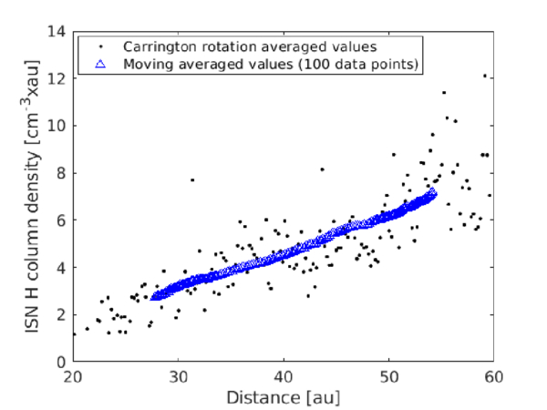
Figure 13. The ISN H column density as a function of distance. The black dots represent the Carrington rotation averaged values, while the open triangles indicate the moving averaged values using 100 data points.
Download figure:
Standard image High-resolution image