Abstract
The large-scale plasma density structure of the extended solar corona is a tracer of the underlying magnetic field configuration and dictates the structure of the solar wind in interplanetary space. Accurate density maps are therefore important to probe the physics of the solar corona and the solar wind, and to improve space-weather forecasting. Density can be estimated from coronagraph observations using solar rotational tomography and is independently provided by global magnetohydrodynamic models. This study compares densities from tomography with the Magnetohydrodynamic Algorithm outside a Sphere (MAS) model across the whole corona over a solar cycle from 2007 to late 2023. The dependence of electron densities on latitude and heliocentric height is compared, with densities in better agreement at equatorial regions and lower heights. The streamer and nonstreamer regions are compared separately, as well as the average width of the streamer belt over the duration of solar cycle 24. The MAS model densities contain more fine-scale detail than those of the tomography, but there is a very good overall agreement in the structure and location of high-density features. In polar regions, where the photospheric magnetic field measurements that drive the MAS simulations present very large uncertainties, the tomographic densities are more accurate. Investigating the accuracy and reliability of these models, and understanding their limitations is crucial. Comparisons with observations highlight their advantages and disadvantages while stressing the importance of observational techniques to help constrain current and future models.
Original content from this work may be used under the terms of the Creative Commons Attribution 4.0 licence. Any further distribution of this work must maintain attribution to the author(s) and the title of the work, journal citation and DOI.
1. Introduction
Information on the large-scale three-dimensional (3D) structure of the solar corona is central to understanding the connection between the corona and the lower solar atmosphere, to interpret observations including in situ spacecraft measurements, to understand the evolution of the large-scale corona over a solar cycle, and to constrain models of the solar wind, including models used in space-weather forecasting. However, mapping this structure directly from observations is challenging due to the line-of-sight (LOS) effect through the optically thin plasma. There is therefore a dependence on the use of models of varying complexity, all based on photospheric magnetic field observations, to probe the coronal and solar wind structure.
The corona is a tenuous, hot (>106 K) plasma consisting of electrically charged ions. As a result, it is optically thin in the visible-light (VL) and extreme-ultraviolet (EUV) spectral regimes, so that the brightness observed at a point on the plane of sky (POS) is the integration of emissions distributed along an extended LOS through the medium. VL and EUV images of the corona are therefore two-dimensional projections of a more complex 3D underlying structure. One of the most effective techniques used to determine the 3D distribution of the coronal plasma in those spectral regimes is solar rotational tomography (SRT). SRT involves observing the corona from different viewpoints, which can be achieved using sequences of images acquired over an adequate time period. For a single observer, this period must span half a solar rotation, although this period may be shortened by using two or more viewpoints with longitudinal separation. For comprehensive overviews of SRT and stereoscopic techniques, see A. M. Vásquez (2016) and M. J. Aschwanden (2011).
SRT techniques have been used extensively since their inception by M. D. Altschuler & R. M. Perry (1972), with many studies improving on this original method. For example, R. A. Frazin (2000) and R. A. Frazin & P. Janzen (2002) developed a more robust method for tomographic inversion from a time series of VL images. R. A. Frazin et al. (2007) presented the first 3D tomographic reconstructions of the coronal electron density from an extended sequence of VL polarized brightness (pB) observations. The study used 2 weeks of images from the Large Angle and Spectrometric Coronagraph (LASCO; G. E. Brueckner et al. 1995) on board the Solar and Heliospheric Observatory (SOHO; V. Domingo et al. 1995). H. Morgan et al. (2009) presented the qualitative solar rotational tomography technique, which uses total-brightness VL observations processed with a suitable background subtraction and a normalizing-radial-graded filter. The method was used to create global maps of the coronal structure at heliocentric heights ≥3 R⊙. One key assumption common to all the aforementioned studies is that of a static corona during the observation period. This assumption is most appropriate during periods of lower solar activity, but breaks down with increasing activity. M. D. Butala et al. (2010) presented the first global reconstruction of the corona using a novel dynamic reconstruction method, with D. Vibert et al. (2016) introducing several new techniques to reduce the effects of coronal dynamics on VL tomographic reconstructions. A novel tomographic technique based on spherical harmonics was developed by H. Morgan (2019, hereafter Paper II), which is discussed in more detail in Section 2.2. The spherical harmonic approach of Paper II has been applied to VL data from 2007 to present, and has allowed an empirical relationship to be found between density and the solar wind speed at 8 R⊙, as well as a relationship with the subsequent acceleration profile in interplanetary space. This approach has enabled a novel boundary condition for solar wind models based on tomography maps rather than magnetic models based on photospheric observations (K. A. Bunting & H. Morgan 2023, 2022; K. A. Bunting et al. 2024). More recent studies involving tomographic techniques to study the solar corona include A. Asensio Ramos (2023), who investigated the application of neural fields for tomographic reconstructions of the VL corona using data from LASCO/C2.
The coronal plasma is constrained and shaped by magnetic field lines originating from deep within the Sun, which permeate throughout the corona and produce the variety of structures and phenomena observed. Understanding the coronal magnetic field is essential for studying the morphology, properties, and dynamics of the solar atmosphere. However, unlike the photosphere where the magnetic fields are routinely measured, it is very difficult to directly measure the magnetic fields in the corona. As a result, theoretical models are required which use the photospheric magnetic field as an inner boundary to simulate the coronal magnetic field configuration. Different techniques have been developed to model the coronal magnetic field based on photospheric magnetic field lower boundary conditions. The simplest approach is the potential field source surface (PFSS) model first developed by K. H. Schatten et al. (1969) and M. D. Altschuler & G. Newkirk (1969). Assuming zero electrical currents in the corona, PFSS models compute the magnetic field in the region from the photosphere to a specified “source surface” where the magnetic field is assumed to be purely radial (typically a heliocentric height of 2.5 R⊙). Due to its simplicity, it is the most commonly used method to model the coronal magnetic field, but there are other models, such as 3D global magnetohydrodynamic (MHD) models, which are computationally more expensive and should provide more accurate results due to including the effects of the plasma on the magnetic field. However, it is also common for studies to use a combination of different models (M. Nedal et al. 2023). Typically, global MHD models can be summarized in two steps: first, the photospheric radial magnetic field is used as the lower boundary condition of the model; and, second, the model advances until the coronal plasma and magnetic fields reach a near equilibrium (P. Riley et al. 2021). However, there are many different methods of producing MHD models which have been used to study various dynamic phenomena, e.g., coronal mass ejections (R. Lionello et al. 2013; T. Török et al. 2018; J. A. Linker et al. 2024; P. Mayank et al. 2024), solar energetic particles (N. A. Schwadron et al. 2014; J. A. Linker et al. 2019; G. Li et al. 2021; E. Palmerio et al. 2024), and flares (J. Muhamad et al. 2017; S. Inoue & Y. Bamba 2021; S. Agarwal et al. 2024; M. González-Servín & J. J. González-Avilés 2024).
Tomographic and stereoscopic techniques are commonly used in conjunction with MHD models to validate the models and place further constraints on the coronal plasma. Furthermore, since tomographic reconstructions are based purely on coronal observations, whereas MHD models are primarily based upon photospheric magnetic field observations, the former should be a more realistic representation of the coronal structure. A. M. Vásquez et al. (2008) demonstrated a validation of two 3D MHD coronal models by comparing density outputs from the models with densities reconstructed using SRT techniques on VL input data for a single Carrington rotation (CR 2029). M. Jin et al. (2012) performed a similar validation study using a 3D, two-temperature, Alfvén-wave-driven global solar wind model and electron density derived from a tomographical inversion of both VL and EUV data. M. Kramar et al. (2014) used a tomographic reconstruction of the 3D coronal electron density from STEREO/COR1 data in both the VL and EUV regimes during a deep minimum in 2008 (CR 2066) to relate the reconstructed 3D density to open/closed magnetic field structures. D. G. Lloveras et al. (2022) applied SRT techniques to both VL and EUV input data to study the 3D structure of the global corona for CRs 2219 and 2223 and compared the SRT outputs with a 3D MHD model. They found that the model densities agreed with the EUV tomography results within 20%, but it overestimated the density obtained using VL tomography by up to 75%. S. T. Badman et al. (2022) investigated constraining global coronal models, namely PFSS, Wang–Sheeley–Arge, and the Magnetohydrodynamic Algorithm outside a Sphere (MAS) models, with multiple independent observables such as EUV observations of coronal hole locations, VL Carrington maps of the streamer belt, and in situ measurements by the Parker Solar Probe and spacecraft at 1 au.
In this study, coronal electron densities are acquired and compared using two methods, the first being an SRT technique based on spherical harmonics and the second being a global 3D MHD model. SRT techniques can be used to provide constraints based on observational information, which is crucial for the future development of MHD models. The structure of this study is as follows. Section 2 summarizes the MHD model (Section 2.1) and SRT technique (Section 2.2). Section 3 shows the results of the comparisons between the model and SRT density maps for various physical parameters such as latitude (Section 3.2) and heliocentric height (Section 3.3), and isolating the streamer (Section 3.4) and nonstreamer (Section 3.5) regions. The study is concluded in Section 4.
2. Method
2.1. MAS MHD Model
The MHD model used in this study is the MAS code, developed by Predictive Sciences Inc.4 (Z. Mikić et al. 1999), which is the main model in the Corona-Heliosphere collection of MHD models (P. Riley et al. 2012). The package is designed to model the global solar corona from the upper chromosphere out to Earth orbit with the coronal model covering the range 1–30 R⊙ and the heliospheric model covering the range 30–215 R⊙. This particular model has been used extensively to model various coronal structures and dynamics (J. A. Linker et al. 2011; R. Lionello et al. 2013; T. Török et al. 2018) as well as forward modeling to predict the topology of the solar corona during total solar eclipses (TSEs; Z. Mikić et al. 2000; Z. Mikić et al. 2018, 2007).
The model takes photospheric magnetogram data as the lower boundary condition and extrapolates the magnetic field. It can use input data from several observatories including the Mount Wilson Observatory,5 Michelson Doppler Imager on SOHO,6 and Helioseismic and Magnetic Imager (HMI; P. H. Scherrer et al. 2012) on the Solar Dynamics Observatory (W. D. Pesnell et al. 2012). The code uses a nonuniform staggered grid, which allows it to resolve smaller-scale structures like active regions while also allowing for coarser grid points over the global scale. Model runs can be requested on the Community Coordinated Modeling Center.7 In the standard “equilibrium” mode of operation, these model results are based on a specific Carrington rotation, i.e., the photospheric magnetic field synoptic map used as an input for the model run is built up from a sequence of observations centered at central meridian over a 27 days period. This inner boundary condition is then supplemented with auxiliary boundary conditions that approximate the plasma density and temperature. Consequently, synthetic observables such as pB and B can be calculated to compare the simulation results with observations.
There are two main model types currently available online: thermodynamic and polytropic. The coronal polytropic model is a 3D MHD model which uses a simple energy equation, whereas the thermodynamic models use a more sophisticated energy equation which includes coronal heating, radiative losses, and thermal conduction. The thermodynamic models use one of two heating models: heating model 1 or heating model 2. Both are an empirical coronal heating model but the former, described in R. Lionello et al. (2009), has three components tailored for active regions, coronal holes, and the quiet Sun where the volumetric heating relies solely on the local parameters of the magnetic field. The latter, heating model 2, features multiple components designed to match the multispectral emission of the corona, much like heating model 1, but in this case the volumetric heating depends on the properties of the surface magnetic field as well. Figure 1 shows a comparison between thermodynamic MAS model outputs for a mid-date of 2008 December 14 at a heliocentric height of 4 R⊙. The top-left and top-right panels show the output when using the thermodynamic model with heating model 1 and 2, respectively, whereas the bottom panel shows the relative difference between both heating models.
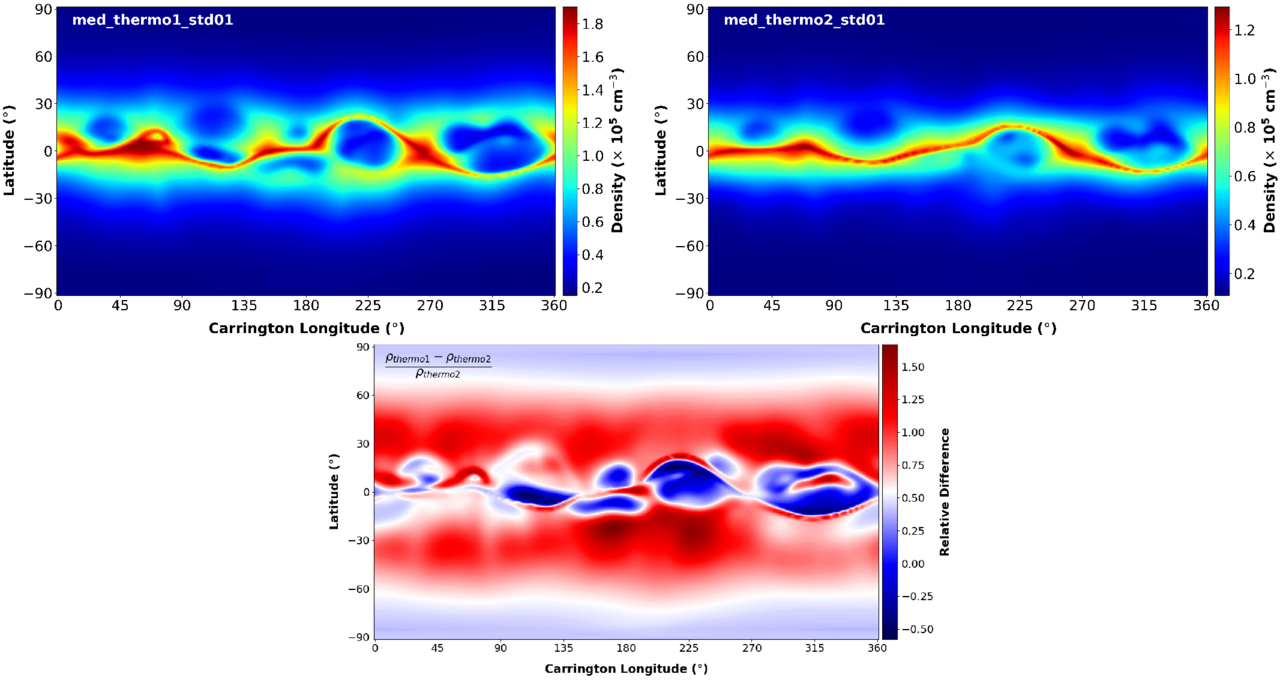
Figure 1. MAS model outputs for a mid-date of 2008 December 14 at a heliocentric height of 4 R⊙. Top left: thermodynamic with heating model 1. Top right: thermodynamic with heating model 2. Bottom: relative difference between both heating models calculated as (ρthermo1 − ρthermo2)/ρthermo2.
Download figure:
Standard image High-resolution imageTable 1 shows the model parameters used in this study along with the dates corresponding to each solar cycle phase. The last date listed in the table, during the very last solar minimum period, corresponds to a TSE. Density maps were compared for each solar cycle phase outlined in Table 1 and the resulting MAS output which most closely resembled the corresponding tomography output in both numerical value and structure was selected for this study. In the case of Figure 1, the model selected for comparison with the tomography density map was model 1 (top-right panel). Figure 1 highlights the importance of selecting the more appropriate MAS model for comparison with the SRT densities. In this case, heating model 1 predicts higher densities overall between ±60° and produces a more similar range of densities with the SRT output than heating model 2. The thermodynamic model has been used for each case study, with the majority using heating model 2. However, heating model 1 was used for both the minimum and ascending phases of the solar cycle as they more closely resembled the tomography density maps for those phases. Solar rotational tomography techniques can provide these constraints and is one of the few ways in which this can be done globally. This study aims to provide this assessment of empirical global MHD models, where results from the MAS model are qualitatively compared with those acquired using the tomography method, as well as observational data from coronagraphs. Several physical parameters were varied, namely latitude, heliocentric height, and solar cycle phase, along with a comparison between the streamer and nonstreamer regions.
Table 1. MAS Parameters for Each Solar Cycle Phase
| Phase | Date | Observatory | Model Type | Heating Model |
|---|---|---|---|---|
| Minimum | 2008 December 14 | MDI | Thermodynamic | 1 |
| Ascending | 2011 August 14 | HMI | Thermodynamic | 1 |
| Maximum | 2014 April 14 | HMI | Thermodynamic | 2 |
| Descending | 2017 February 13 | HMI | Thermodynamic | 2 |
| TSE | 2020 December 14 | HMI | Thermodynamic | 2 |
Download table as: ASCIITypeset image
2.2. Solar Rotational Tomography
H. Morgan (2015, hereafter Paper I) presents a description of data preprocessing and calibration techniques for the LASCO C2 instrument on SOHO and the SECCHI COR2 instrument on board the STEREO A and B spacecraft. These processed and calibrated coronagraph data are then used as the input for a novel SRT method based on spherical harmonics, presented in Paper II, which reconstructs the coronal electron density. This method represents the density as a weighted combination of spherical harmonic functions in longitude and latitude, with independent profiles defined at discrete radial heights. The inversion process minimizes the difference between observed and modeled white-light brightness, under the assumption of a static corona over a 2 week observational window. Regularization is applied to suppress unphysical small-scale variations and to balance spatial resolution with stability, with additional weighting based on estimated noise in the data. To improve the accuracy of reconstructed streamer structures, a postprocessing step narrows overly broad high-density features based on a best-fit correction.
This method is used to obtain density maps of the coronal electrons at heliocentric distances from ≈ 3 R⊙ to 8 R⊙, and maps are produced at ≈2 days increments, starting at a mid-date of 2007 March 17, resulting in thousands of maps, which can be freely downloaded from the Aberystwyth University archive.8 Initial results of the method are presented in H. Morgan & A. C. Cook (2020, hereafter Paper III) as well as further developments to the method. Each tomography map is generated using approximately 2 weeks of COR2A data, meaning it represents a static reconstruction of the coronal density over a ±1 week period. For each mid-date, a set of nine maps is created at heliocentric distances between 4 and 8 R⊙ at ≈0.5 R⊙ increments. A coronal electron density map produced using the SRT technique is shown in Figure 2 for a mid-date of 2008 December 14 and a heliocentric height of 4 R⊙. There is a very good agreement between Figures 1 and 2, primarily the densities produced using the thermodynamic output with heating model 2. The numerical values differ between the outputs, but the overall location of high-density structures and the width of the streamer belt agree well.
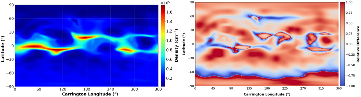
Figure 2. Left: example of a coronal electron density map produced using the SRT method for a heliocentric height of 4.0 R⊙ at a mid-date of 2008 December 14 in Carrington longitude–latitude coordinates. Right: relative difference between the SRT output and the MAS thermodynamic with heating model 1 outputs. The difference is calculated as (ρMAS − ρSRT)/ρSRT.
Download figure:
Standard image High-resolution image3. Results and Discussion
3.1. Qualitative Overall Comparison
Figure 3 shows a comparison of coronal electron density maps produced using SRT (left column) and the MAS model (right column) at a heliocentric distance of 4 R⊙ for dates during each phase of the solar activity cycle. The maps span the entirety of solar cycle 24 (2008–2019) and the start of solar cycle 25 (2020) with each phase separated by ≈3 yr. The minimum phase of solar cycle 25 coincided with the TSE on 2020 December 14, thus, to avoid confusion with the minimum of solar cycle 24, this minimum phase is labeled as the TSE phase.
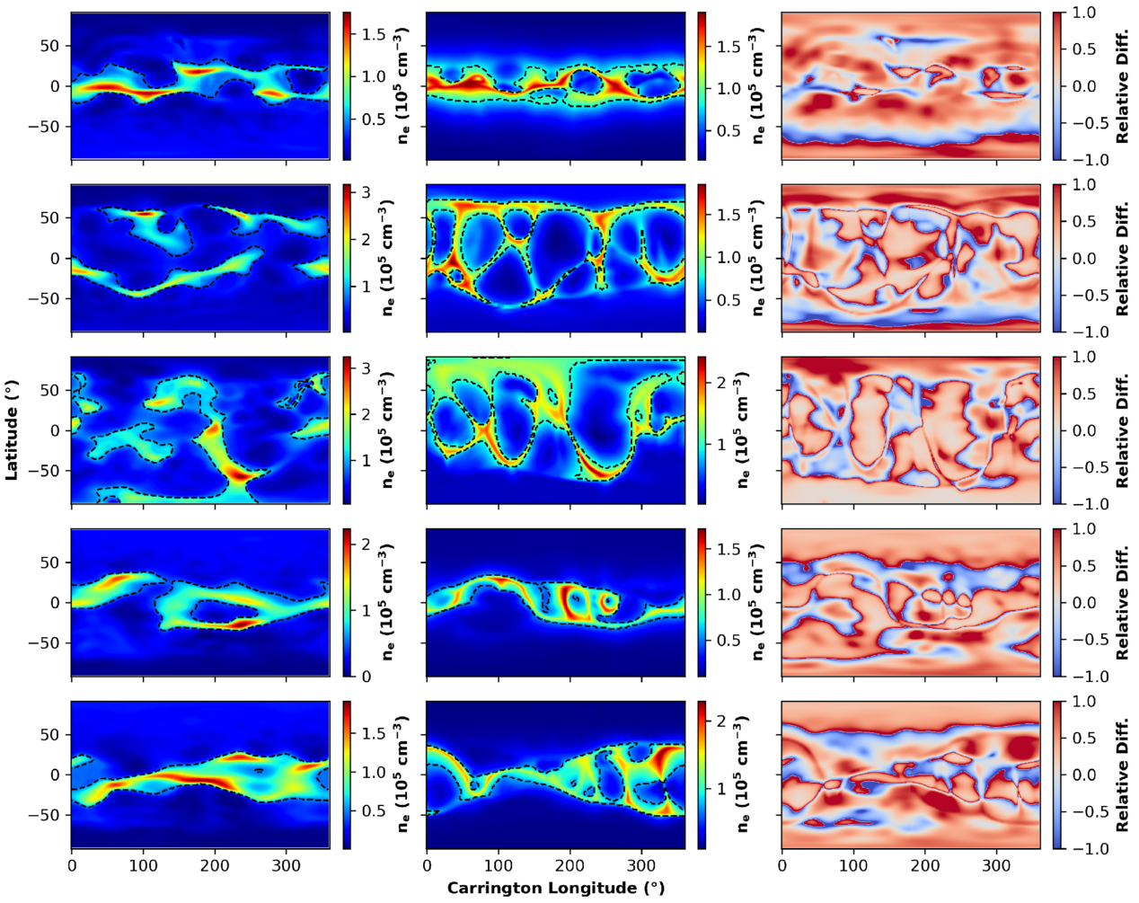
Figure 3. Coronal electron densities produced using the SRT technique (left column) and the MAS model (middle column) at a heliocentric height of 4 R⊙ for dates during each phase of the solar activity cycle; see Table 1 (top to bottom: minimum, ascending, maximum, descending, TSE). The streamer regions, defined as regions where the density is greater than 1.5 times the mean global density of each map, are represented by the dashed black contours, and the color bars in the MAS outputs have been normalized to match those from the SRT technique outputs in order to make qualitative comparisons of large-scale structures easier. Right column: relative difference between SRT and MAS outputs at each stage of the solar cycle, calculated as (ρMAS − ρSRT)/ρSRT.
Download figure:
Standard image High-resolution imageFigure 3 shows that there is good overall agreement between the tomography and the MAS model maps. Despite the fact that the tomography process involves regularization which may remove finer-scale details that are visible in the MAS outputs, the overall structure of the maps are very similar. For example, the current sheet, which is more apparent at periods of lower solar activity, can be traced in both the tomography and MAS outputs at similar locations. Furthermore, pockets of lower-density regions can be seen in similar locations in both outputs; for example, at solar minimum between 20° and −10° in latitude, there are two pockets of lower density at Carrington longitudes of ≈210°–240° and ≈300°–350° in both outputs.
The right column in Figure 3 shows the relative difference between both outputs determined using the formula in the bottom left of each panel. These figures reinforce the good agreement between both outputs overall, while also highlighting localized regions of higher differences. During the solar minimum, descending, and TSE phases the differences tend to occur at lower latitudes, whereas during the ascending and maximum phases the differences tend to be seen at higher latitudes. Both the tomography and MAS outputs also show the varying of the streamer belt’s width as a function of solar cycle phase very well, with the streamer belt narrower and more contained at times of lower solar activity and much wider and less defined at times of higher solar activity. However, the widths of the streamer belts in the MHD model do not always agree with those of the tomography maps. An example of this difference can be seen during the TSE phase in Figure 3 (bottom row), where the MHD model shows a much wider streamer belt, particularly between 0°–60° and 270°–360° Carrington longitude. In Section 3.4, the streamer regions are discussed in more detail. Since the MAS model takes observational measurements of the radial component of the photospheric magnetic field (Br), usually in the form of a LOS photospheric magnetogram, as its input, it cannot accurately measure Br at higher latitudes due to projection effects. Therefore, it uses a fitting procedure to estimate Br in the polar regions, which is likely why the MAS outputs appear much smoother in the polar regions than the tomographic equivalent.
For the period of maximum activity shown in the third panel of Figure 3, the MAS model output shows much finer-scale structure than the tomography, but there is a good agreement in the position of higher-density structures and lower-density pockets between the two maps. For example, the high-density structure at ≈−30° to −60° latitude and ≈210°–240° longitude is agreed upon very well in both maps, with some obvious discrepancies in the polar regions. For example, the tomography map indicates that there is a relatively high-density structure visible in the southern polar region, extending from ≈30° to 240° in longitude at a latitude of ≈−80°, which is not at all visible in the MAS output (see Section 3.6). Furthermore, there is a region in the northern hemisphere of the MAS output that suggests a high-density region spanning from ≈0° to 200° in Carrington longitude and from ≈60° to 90° in latitude, which is not seen in the SRT output. This is further shown by the relative difference plot showing a large relative difference between both outputs, which is most probably due to the issue of obtaining accurate photospheric radial magnetic field data at such high latitudes.
3.2. Quantitative Latitudinal Comparison
Figure 4 shows a comparison of coronal electron densities derived from the SRT technique (red) and the MAS model (blue) averaged over longitude at each latitude for heliocentric heights of 4 (left column) and 8 R⊙ (right column) over each phase of the solar activity cycle. There is a reasonably good agreement between the SRT output and the MAS model in terms of the numerical values of the densities in the equatorial regions, and the position of the higher-density structures, particularly at a heliocentric height of 4 R⊙. However, there are also some discrepancies between both outputs, particularly at a heliocentric height of 8 R⊙, where the SRT densities are greater than the MAS densities during most phases of the solar cycle.
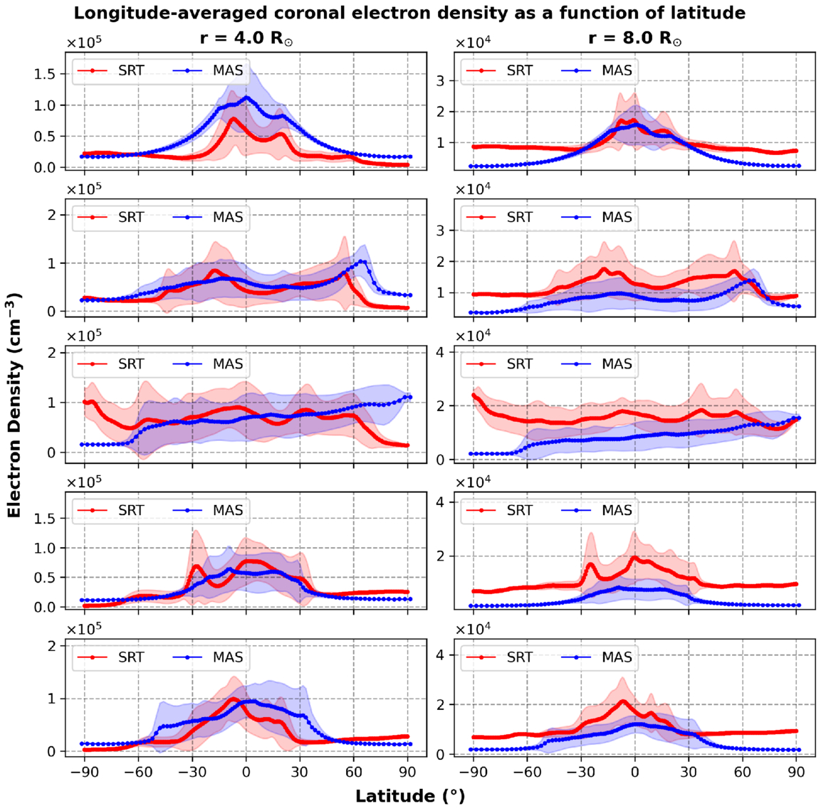
Figure 4. Coronal electron densities derived from the SRT maps (red) and the MAS model (blue) averaged over longitude at each latitude for heliocentric heights of 4 R⊙ (left column) and 8 R⊙ (right column) for dates during each phase of the solar activity cycle; see Table 1 (top to bottom: minimum, ascending, maximum, descending, TSE). The red and blue shaded areas represent the tomography and MAS model standard deviations, respectively.
Download figure:
Standard image High-resolution imageAt a heliocentric height of 4 R⊙, there is generally a good large-scale agreement between the output of MAS and the SRT results, except during the solar maximum phase where short-timescale dynamic processes are at their most frequent, which strongly affects both methods. In the case of SRT, the smaller-timescale dynamic phenomena cannot be reconstructed since the input requires 2 weeks of VL observations and assumes a static corona during that time. In the case of an MHD model, the 27 days worth of data that composes the synoptic magnetogram used as input is constructed with measurements taken at different times. As a result, there will inevitably be more differences between both outputs during solar maximum, as well as differences from the true coronal density. At 8 R⊙, there is a reasonably good agreement between the MAS and SRT outputs during the minimum and TSE phases, as well as at equatorial streamer belt regions (±30°). However, during the ascending, maximum, and descending phases the MAS model underestimates the SRT-reconstructed density.
During solar minimum at 4 R⊙, the SRT output has two main peaks near latitudes −10 and +20°, whereas in the MAS output the peaks are less apparent. The MAS densities are greater at latitudes between ±60° and have a shallower decrease with increasing latitude than the SRT output. There is a good agreement between both outputs at higher latitudes with both densities converging to a polar density of ≈0.2 × 104 cm−3. However, at 8 R⊙, there is a much closer agreement at equatorial latitudes but an increased difference at latitudes greater than ±30°, resulting in a difference of ≈0.6 × 104 cm−3 at polar latitudes.
During the ascending phase at 4 R⊙, there is a good agreement between the magnitudes of the two output densities, although there is a slight discrepancy at northern latitudes above ≈60° where the MAS output reaches a maximum of ≈1.0 × 105 cm−3 at a latitude of 65°, whereas the SRT output reaches a maximum density of ≈0.8 × 105 cm−3 at 55°. Both SRT and MAS densities then decrease with increasing latitude until they reach densities of ≈0.1 × 104 cm−3 and 0.3 × 104 cm−3, respectively. At 8 R⊙, there is a large discrepancy between the two densities throughout the latitude range from −90° to +60°, where there is a reasonable agreement only during the interval +60° to +80°.
During solar maximum at 4 R⊙, there is a reasonably good agreement between the magnitude of both output densities at equatorial latitudes but a disagreement in the position of density peaks, particularly at around −5° latitude. Furthermore, there is a large disagreement at latitudes south of ≈−60°, which is investigated in more detail in Section 3.6. At high northern latitudes, the SRT density decreases with increasing latitude, as is expected, but the MAS output fails to reproduce the density peaks clearly seen in the SRT maps near latitudes ≈−5°, +30°, and +55°. At 8 R⊙, and similar to the ascending phase, there is a large difference between both output densities from −90° to ≈−70°.
As the solar activity decreases from maximum, there is a better agreement between both outputs, both in magnitude and structure, across all latitudes, which is particularly apparent at 4 R⊙. For example, from ≈+20° to +50°, there is a very good agreement between both outputs, as well as a good agreement in the latitude of the peak at −25°. However, the MAS model predicts a peak at ≈−10°, whereas the SRT density peaks at ≈+5°. At 8 R⊙, the MAS densities are much lower than the SRT densities at each latitude, with the maximum density from the MAS output approximately the same as the minimum density from the SRT output.
There is a reasonably good agreement during the TSE phase at 4 R⊙, as well, particularly at equatorial latitudes. The densities from ≈−20° to +40° in latitude agree well in their structures but are shifted in latitude by 10°–15°, with both SRT peaks at −5° and +15° also present in the MAS output but at +5° and +35°. Furthermore, there is a reasonably good agreement at higher latitudes similar to that seen during the minimum phase. At 8 R⊙, there is a closer agreement between the SRT and MAS outputs at southern latitudes, whereas during the solar minimum phase, the inverse is true and the northern densities are closer in magnitude between both outputs. Furthermore, there also seems to be a difference of ≈5°–10° in latitude between the peaks present in both outputs.
3.3. Height Dependence
Figure 5 shows the average global coronal electron density produced using SRT (red) and the MAS model (blue) as a function of increasing heliocentric height for each phase of the solar cycle (left column). The red and blue shaded regions correspond to 1 standard deviation for the SRT and MAS outputs, respectively. Model fits for the average SRT (red) and MAS (blue) global density radial profiles are also given. It also shows the difference in the average streamer densities at each heliocentric height expressed as a percentage, with its associated error determined by error propagation (right column). The magnitude of the SRT densities gradually increases from solar minimum to maximum and then decreases toward the TSE phase around the minimum of the next solar cycle. The same pattern is seen in the MAS model output but to a lesser extent than the SRT. Furthermore, at times of lower solar activity, the average global densities agree better at greater heliocentric heights, whereas the inverse is true at times of higher solar activity.
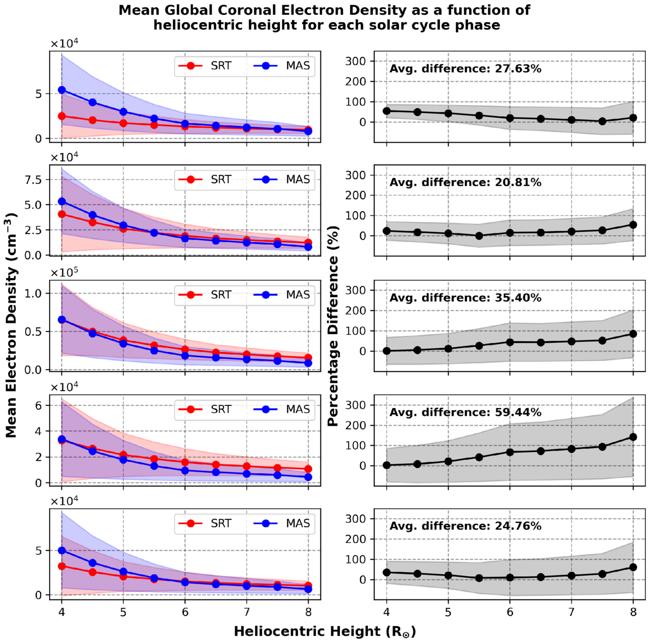
Figure 5. Left column: comparison of average coronal electron densities using SRT (red) and the MAS model (blue) as a function of heliocentric height for dates during each phase of the solar activity cycle (top to bottom: minimum, ascending, maximum, descending, TSE). The red and blue shaded regions give the standard deviations of the SRT and MAS model, respectively. Right column: percentage difference between both outputs at each heliocentric height as well as the associated error (shaded region) determined by error propagation. The difference is calculated as (ρSRT − ρMAS)/ρMAS, and the average percentage difference between the two outputs is also displayed in the top-left corner of each panel.
Download figure:
Standard image High-resolution imageDuring solar minimum, there is a noticeable difference (≈50%) in the average global density between the SRT and MAS outputs at 4 R⊙, with a MAS global density of ≈5.5 × 104 cm−3 and an SRT global density of ≈2.5 × 104 cm−3. However, as heliocentric height increases, the two outputs tend to agree better, particularly above 7 R⊙. The standard deviation in the MAS output is also greater than the SRT output at each heliocentric height, and the average percentage difference between both output densities across all heights is ≈27%. During the ascending phase, there is a better overall agreement between the two outputs in comparison with the minimum phase, resulting in an average percentage difference of ≈20% across all heights. The MAS average global density is higher than the SRT output at lower heights (4–5 R⊙), with a good agreement at 5.5 R⊙, and the SRT density is greater than the MAS density beyond that height. The SRT standard deviation is greater during this phase, which is expected since the method’s reliability decreases with increasing solar activity.
At solar maximum, the two outputs agree very well at lower heliocentric heights but diverge with increasing heliocentric height, as quantified in the corresponding percentage difference panel. Despite this, the overall agreement across all heights is good, with an average difference of ≈35%. This level of agreement is notable given not only the limitations of the SRT method during solar maximum but also those inherent to the MAS model. For instance, the photospheric magnetograms used as inputs for the model combine individual magnetograms taken over the course of a full Carrington rotation, potentially misrepresenting dynamic features that evolve over more rapid timescales. Additionally, uncertainties in the radial magnetic field measurements can propagate through the model, further affecting the output densities.
The same trend is also seen during the descending phase but to a greater extent, where the densities at lower heights agree better, then the differences between the two outputs increase with increasing radial height. The average percentage difference across all heights during this phase is ≈56%, which is considerably greater than any other phase. Finally, during the TSE phase, the density profiles from both outputs are similar in structure to those seen during the ascending phase, with higher MAS densities at lower heliocentric heights and higher SRT densities at higher heights. This results in an average percentage difference across all heights of ≈24% during the TSE phase.
3.4. Streamer Belt
In Figure 3, the streamer regions are shown as dashed black lines and are defined as regions where the density is greater than 1.5 times the mean global density at each height. As the solar cycle progresses, the structure of the streamer belt becomes less coherent and more complex, before becoming more structured once again by the end of the cycle. There is a discrepancy between the width of the streamer belt in some instances, primarily in the TSE phase (bottom row). However, the streamer belts given by the SRT and MHD model generally show very good agreement. For example, at solar maximum, there is a high-density feature between −20° to –60° latitude and 200° to 280° Carrington longitude which is seen in both outputs, exhibiting similar density values, shape, and location. Figure 6 shows the average streamer densities in the same manner as Figure 5.
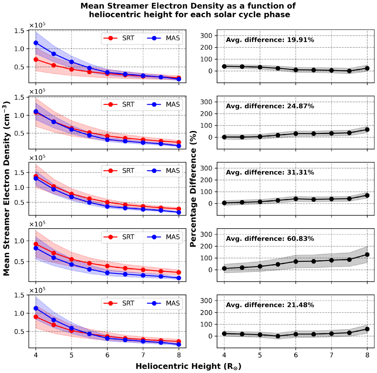
Figure 6. Left column: comparison of mean streamer region electron densities using SRT (red) and the MAS model (blue) as a function of heliocentric height for dates during each phase of the solar activity cycle (top to bottom: minimum, ascending, maximum, descending, TSE). The red and blue shaded regions give the standard deviations of the SRT and MAS model, respectively. Right column: percentage difference between both outputs at each heliocentric height as well as the associated error (shaded region) determined by error propagation. The difference is calculated as (ρSRT − ρMAS)/ρMAS, and the average percentage difference between the two outputs is also displayed in the top-left corner of each panel.
Download figure:
Standard image High-resolution imageDuring solar minimum, the average MAS streamer region density at 4 R⊙ is double that of the average SRT output. However, as the radial height increases, the streamer densities from both outputs agree increasingly well, particularly from 7 to 7.5 R⊙, resulting in an average percentage difference across all heights of ≈20%. Additionally, the standard deviations of both outputs become smaller at higher radial heights, with comparable standard deviations between the two outputs from 6 to 7.5 R⊙. During the ascending phase, there is a particularly good agreement between both outputs at lower radial heights (≤5 R⊙), resulting in an average difference of ≈25% across all heights. The densities from both outputs then diverge beyond 5.5 R⊙, resulting in a percentage difference of ≈65% at 8 R⊙.
During solar maximum, the average SRT and MAS streamer densities agree well overall, but particularly below 5 R⊙ where the densities differ by only ≈5%–15%, whereas the average difference between both outputs increases with increasing heliocentric height up to ≈68% at 8 R⊙. As discussed previously, the reliability of both methods is affected by the increased solar activity—more accurately, the increase in rapidly evolving dynamic phenomena. Despite this, the overall agreement between the SRT and MAS densities, particularly at lower heights, suggests that large-scale coronal structures remain sufficiently stable to allow meaningful comparisons between both outputs, even during solar maximum.
During the descending phase, the average percentage difference is greater than during the selected solar maximum period, with a value of ≈145% at 8 R⊙. The densities agree reasonably well at low heliocentric heights but diverge beyond 5 R⊙. The descending phase selected for this study may have featured a more dynamic or less stable corona than the solar maximum period analyzed, underscoring the importance of coronal evolution on comparisons between models and observation. Broader statistical comparisons across multiple rotations during each solar phase would be needed to assess whether this trend holds more generally, but that is beyond the scope of this study. Finally, during the TSE phase, the average MAS densities are greater than the SRT densities at lower radial heights, are comparable at 5.5 R⊙, then decrease faster with increasing height beyond that. The average percentage difference across all heights is ≈21%, which is in good agreement with the first minimum phase at ≈20%.
Figure 7 gives examples of SRT (left column) and MAS (right column) density maps where the longitude-averaged minimum and maximum latitude of the streamer region are also shown. The top panels show density maps for a mid-date of 2019 December 22, corresponding to solar minimum, whereas the bottom panels show density maps for a mid-date of 2014 April 19, corresponding to solar maximum. The dashed white lines show the average upper and lower limits of the streamer belt in each case, which are determined by calculating the maximum and minimum latitudes of the belt at each longitude and computing their average. The difference between these two average values gives the average width of the streamer belt for the corresponding density map.
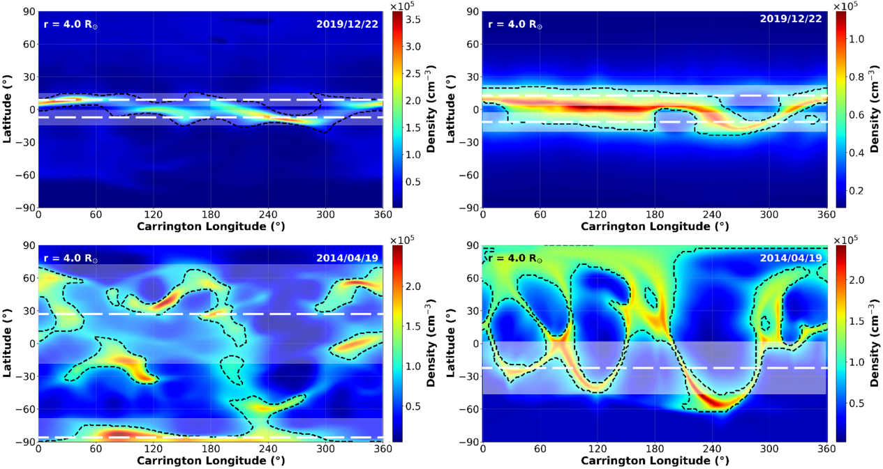
Figure 7. Examples of SRT (left column) and MAS (right column) density maps for mid-dates of 2007 March 21 (top row) and 2014 April 19 (bottom row) representing periods of minimum and maximum solar activity, respectively. The dashed white lines show the longitude-averaged minimum and maximum latitude of the streamer region. The surrounding shaded regions represent 1 standard deviation above and below each limit. The heliocentric height and mid-date for each map is displayed in the top-left and top-right corners of each panel, respectively, and the streamer regions are also highlighted by the dashed black contour.
Download figure:
Standard image High-resolution imageAs expected, the streamer belts in both outputs are narrower and more coherent at solar minimum than at solar maximum, with far fewer high-density features seen outside the dashed white lines during this time. The shaded white regions surrounding the dashed white lines show 1 standard deviation above and below, which is used in this instance as an estimate for the uncertainty; as expected, the upper and lower limits are much more defined during solar minimum. At solar maximum, the standard deviations from both the SRT and MAS outputs are very large, and as a result represent a much greater uncertainty in both the position of each limit and the overall width of the streamer belt at that time. Furthermore, the average upper limit of the streamer belt at solar maximum given by the MAS output was greater than 90°, hence why it is not visible in the plot. This further demonstrates that MHD models reliant upon photospheric magnetograms as inputs are unreliable at high latitudes.
The average streamer belt width was calculated at 4 R⊙for every tomography map available between 2007 and late 2023, as well as at each Carrington rotation for the MAS model. The results are shown in Figure 8, where the red and blue data points represent the SRT and MAS model outputs, respectively. The shaded region and the error bars represent the standard deviation for the SRT and MAS model output widths, respectively. As expected, the average streamer belt width is largest in 2014 and 2024, at the peak of the solar activity cycle, and is the smallest during solar minimum. The data gap in the SRT output from early 2014 to late 2015 is a result of the STEREO-A COR2 spacecraft passing behind the Sun. The MAS streamer belt widths agree well with those of the SRT, with all data points and their errors overlapping for each solar cycle phase. The same solar cycle trend seen in the tomography is also seen in the MAS model outputs, where the streamer belt is narrower and more coherent at periods of lower solar activity and wider with greater standard deviations at periods of increased activity. There is a very good agreement between the two outputs throughout the solar cycle, despite the SRT technique’s limitations during active periods. The standard deviation of both methods is greatest during solar maximum, but the MAS model widths have a much greater standard deviation from 2016 to 2022 than the SRT method. There is also a period of time around 2015 where the MAS model estimates a much wider streamer belt than the SRT method does. Despite these points, the agreement between the two methods is excellent.
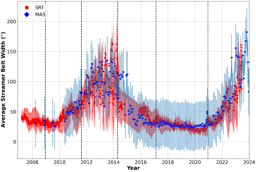
Figure 8. Average streamer belt width at 4 R⊙ calculated for each SRT map available between 2007 and 2023 (red), with the shaded region representing its standard deviation. The average streamer belt width calculated from the MAS model outputs for each Carrington rotation available is also shown (blue), with corresponding standard deviations shown as vertical error bars. The vertical dashed black lines represent the dates used throughout this study, and the data gap in the tomography from early 2014 to late 2015 is due to the STEREO-A spacecraft moving behind the Sun.
Download figure:
Standard image High-resolution image3.5. Nonstreamer Regions
Figure 3 also shows the nonstreamer regions, where the data shown are less than or equal to 1.5 times the mean global electron density for that phase of the solar cycle. These results show considerably more discrepancies between them in comparison to those acquired for the streamer belts. The density maps for times of lower solar activity seem relatively similar, but those for solar maximum, for example, are very different. One key difference to note is at solar minimum (top row), where the MAS model suggests more uniform and homogeneous densities at higher latitudes, most probably as a result of the aforementioned interpolation procedure which is used to estimate the magnetogram data at high latitudes. The SRT output seems to suggest far more variation and finer-scale features in these polar regions than the corresponding MAS output.
Figure 9 shows the average nonstreamer densities using SRT (left column) and the MAS model (right column) as a function of increasing heliocentric height for each phase of the solar cycle. Similar to Figure 6, both methods produce densities which are lower during solar minimum and higher at solar maximum. During solar minimum, the average MAS nonstreamer density at 4 R⊙ is ≈3.75 × 104 cm−3, whereas the equivalent average SRT density is much lower at ≈1.6 × 104 cm−3. At 6.5 R⊙, the two outputs produce very similar average densities, whereas above that height the SRT average densities are higher than the MAS outputs. The average densities found during the ascending phase also follow this similar pattern. In fact, this trend—where the MAS average densities are greater at lower radial heights, whereas the inverse is true at higher radial heights—is seen throughout each stage of the solar cycle. The percentage difference during the minimum and ascending phases is also very similar (≈28%).
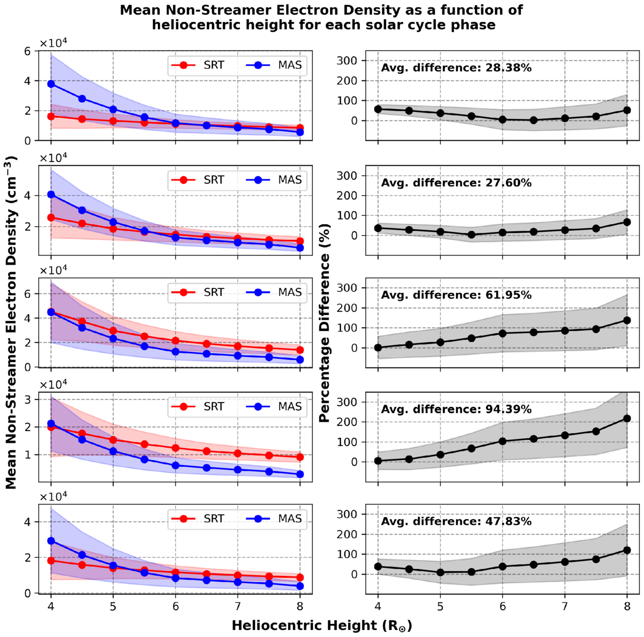
Figure 9. Left column: comparison of mean nonstreamer region electron densities using SRT (red) and the MAS model (blue) as a function of heliocentric height for dates during each phase of the solar activity cycle (top to bottom: minimum, ascending, maximum, descending, TSE). The red and blue shaded regions give the standard deviations of the SRT and MAS model, respectively. Right column: percentage difference between both outputs at each heliocentric height as well as the associated error (shaded region) determined by error propagation. The difference is calculated as (ρSRT − ρMAS)/ρMAS, and the average percentage difference between the two outputs is also displayed in the top-left corner of each panel.
Download figure:
Standard image High-resolution imageDuring solar maximum, however, the average SRT nonstreamer density at 4 R⊙ agrees very well with that of the MAS output (≈4.5 × 104 cm−3). However, as heliocentric height increases, the two outputs differ from each other, with the MAS densities decreasing more rapidly than those from the SRT, resulting in a percentage difference of ≈140% at 8 R⊙. However, similar to the streamer regions, the greatest disagreement between the two outputs is seen during the descending phase, with an average percentage difference of ≈79% across all heights. There is a relatively good agreement between both outputs at low heliocentric heights, but above 5 R⊙ the difference between the two increases greatly, resulting in a percentage difference of ≈190% at 8 R⊙. Finally, during the TSE phase, the percentage difference between both outputs has decreased to ≈48%, but it is still high relative to the percentage difference from the first minimum phase (≈28%). Furthermore, the MAS densities are nearly double the SRT densities at 4 R⊙, but as radial height increases the MAS densities decrease more sharply than the SRT densities, which is over double the MAS density at 8 R⊙.
3.6. Case Study: Streamer of 2014 April 14
The statistical discrepancies observed between the SRT output and the MAS model may arise from specific coronal features that are not present in the MAS model output, particularly at higher latitudes. This section focuses on one such feature—a high-latitude coronal streamer—that is visible in LASCO/C2 observations over the period of ≈3 weeks. As a result, it is very well reconstructed by the SRT, but does not appear in the MAS model output. Figure 10 shows these VL images from the LASCO C2 instrument on board SOHO during 2014 April. Since the SRT method requires a minimum of half a Carrington rotation (≈14 days) of observation to create one density map, for a feature to appear in the resulting maps it should be present and fairly stable over this period. We select for discussion a streamer seen near the south pole at a position angle of ≈158° (measured counterclockwise from the north pole) on 2014 April 7 (left), which can be seen in the coronagraph data a week later on April 14 (middle) at a position angle of ≈171°. It can also be seen on April 21 (right) at a position angle of ≈174°, and the streamer is visible in the SRT map.
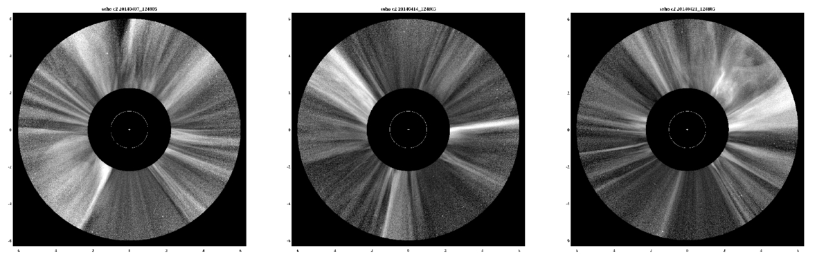
Figure 10. LASCO/C2 observations of the VL corona on 2014 April 7 (left), 2014 April 14 (middle), and 2014 April 21 (right). We highlight here a streamer seen in the southeastern region of the lower corona in all three images. To enhance structural detail, the images have been processed with the normalizing-radial-graded filter (H. Morgan et al. 2006) and multiscale Gaussian normalization (H. Morgan & M. Druckmüller 2014).
Download figure:
Standard image High-resolution imageFigure 11 shows both the observed (top panel) and reconstructed (middle panel) pB of the solar corona at a heliocentric height of 4 R⊙ and a mid-date of 2014 April 14. The observed pB is the input data upon which the tomography maps are based, whereas the reconstructed pB is determined by inverting the SRT densities. The bottom panel is a histogram of the pixel-to-pixel ratio of the reconstructed and observed pB that shows a slightly right-skewed distribution (0.670) with a similar mean (1.037) and median (1.025). There is also a Pearson correlation coefficient of 0.771, indicating a good agreement between the observed and reconstructed pB. Further evidence of a good agreement between the two plots is shown in Figure 12, giving confidence that the density structure in the SRT map is dependable. Despite a very active corona at the time of observation, the SRT method holds up well in a qualitative comparison. Figure 12 shows a line profile comparison between the observed and reconstructed pB taken at the mid-date of Figure 11, shown as black and red profiles, respectively. The reconstructed pB from the SRT method agrees very well with the observed pB, particularly in the southern polar region where the streamer is present. There is a relatively good agreement between the observed and reconstructed pB at position angles of ≈90° and ≈300°–330°, as well as at ≈180° where the streamer of interest is present. However, the pB peak at a position angle of ≈45° has not been well reconstructed by the SRT method, as well as the two peaks at ≈220 and 260°. Despite this, the SRT output has accurately represented the true coronal pB.
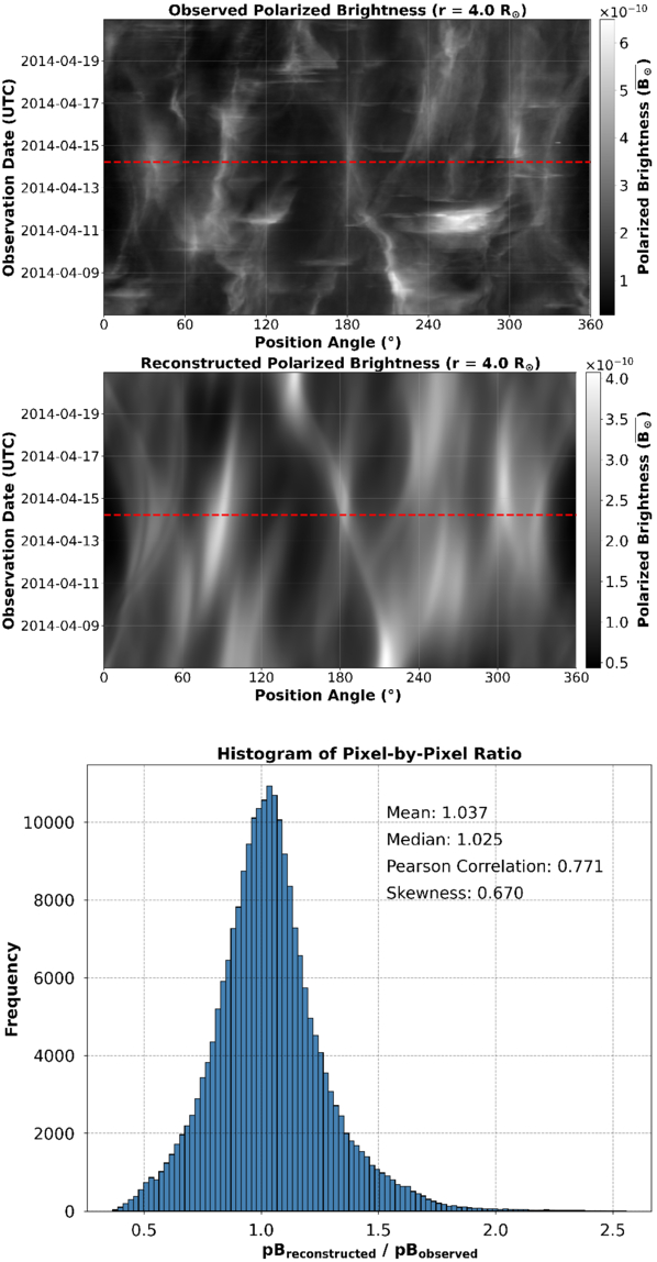
Figure 11. Observed (top) and reconstructed (middle) pB maps of the corona at a heliocentric height of 4.0 R⊙ at a mid-date of 2014 April 14. The data are expressed in units of mean solar brightness and are shown as functions of position angle counterclockwise from solar north. The horizontal dashed red line indicates the mid-date of this time period. A histogram of the pixel-by-pixel ratio of reconstructed and observed pB is also shown (bottom panel) along with its associated mean, median, skewness, and Pearson correlation coefficient.
Download figure:
Standard image High-resolution image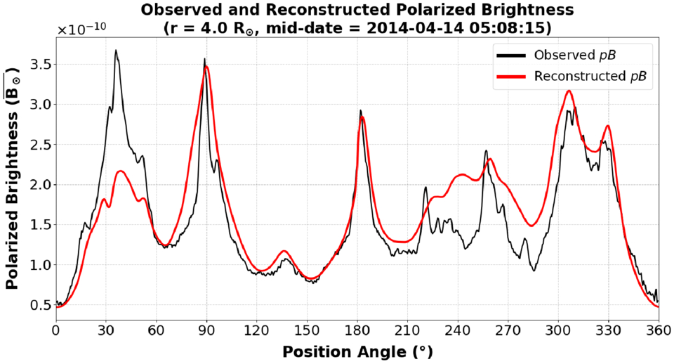
Figure 12. Line profile comparison of the observed (black) and reconstructed (red) pB of the corona at a heliocentric height of 4.0 R⊙ taken at a mid-date of 2014 April 14 (red dashed line in the top and middle panels of Figure 11). The data are expressed in units of mean solar brightness and are shown as functions of position angle counterclockwise from solar north.
Download figure:
Standard image High-resolution image4. Conclusions
The MAS model that agreed best with the SRT was the thermodynamic model, which was to be expected since it uses a more sophisticated energy equation than the polytropic model, including coronal heating, radiative losses, and thermal conduction. Generally, there is good agreement between the density maps produced using the SRT method and those produced using the MAS model. However, there are some cases where the SRT maps show features which are not visible in the MAS outputs, particularly toward polar latitudes. Two reasons can explain this. First, the SRT method is most accurate at the poles since there are uninterrupted observations along the LOS through both polar regions. The second reason originates from the difficulty in obtaining any meaningful magnetic field observations of the solar poles, which consequently affects the ability of MHD models to extrapolate the polar magnetic fields. The densities produced using the SRT method can be verified using the observed and reconstructed pB, which agree well throughout the solar cycle. The densities produced by the two methods typically agree well over a solar cycle, though there are more discrepancies between the two during periods of increased solar activity. There is also a disagreement in nonstreamer densities as heliocentric height increases, with the MAS model densities decreasing too quickly compared with the SRT densities. There is a good overall agreement between the tomography and MAS model outputs for the streamer regions, and the average width of the streamer belt agrees very well between the two methods. The streamer belt is narrow and more coherent in the density maps at periods of lower solar activity and widens to cover a broader latitude range during solar maximum, and this trend is also seen in the MAS outputs. Global 3D MHD models play an important role in understanding solar phenomena, both in the short and long term. As a result, the accuracy and reliability of these models is most crucial, with comparisons such as this study highlighting their advantages and disadvantages as well as stressing the importance of observational techniques to help place physically derived constraints upon both current and future models.
Acknowledgments
The STEREO/SECCHI project is an international consortium of the Naval Research Laboratory (USA), Lockheed Martin Solar and Astrophysics Lab (USA), NASA Goddard Space Flight Center (USA), Rutherford Appleton Laboratory (UK), University of Birmingham (UK), Max-Planck-Institut für Sonnen-systemforschung (Germany), Centre Spatial de Liege (Belgium), Institut Optique Théorique et Appliqúee (France), and Institut d’Astrophysique Spatiale (France). This research used version 5.1.2 (doi:10.5281/zenodo.10927245) of the SunPy open source software package (The SunPy Community et al. 2020). L.E. and H.M. acknowledge studentship funding from the Coleg Cymraeg Cenedlaethol to Aberystwyth University that made this work possible. H.M. acknowledges STFC grant No. ST/V00235X/1. The authors at PSI gratefully acknowledge support from NASA (grants Nos. 80NSSC20K0695, 80NSSC20K1274, 80NSSC20K1285, 80NSSC22K0893, 80NSSC23K0258, and 80NSSC24K1108), the PSP WISPR contract NNG11EK11I to NRL (under subcontract N00173-19-C-2003 to PSI), and NSF’s PREEVENTS program (grant No. ICER-1854790). Coronal electron densities obtained by solar rotational tomography can be downloaded from https://solarphysics.aber.ac.uk/Archives/tomography/. The Magnetohydrodynamic Algorithm outside a Sphere (MAS) model was developed by Predictive Science Inc (https://www.predsci.com/corona/model_desc.html).
Facility: SOHO - Solar Heliospheric Observatory satellite (LASCO).
Software: SunPy (The SunPy Community et al. 2020), pyhdf (https://pypi.org/project/pyhdf/).
Author Contributions
L.E. wrote the main manuscript text and performed the data analysis and processing. H.M. developed the tomography method, contributed to the data analysis, and reviewed the manuscript. P.R. and J.L. are developers of the MAS model, provided expertise, and reviewed the manuscript.
Footnotes
- 4
- 5
- 6
- 7
- 8