Abstract
We review the recent theoretical and experimental progress regarding the generalized hydrodynamics (GHD) behavior of the one-dimensional (1D) Bose gas with contact repulsive interactions, also known as the Lieb–Liniger gas. In the first section, we review the theory of the Lieb–Liniger gas, introducing the key notions of the rapidities and of the rapidity distribution. The latter characterizes the Lieb–Liniger gas after relaxation and is at the heart of GHD. We also present the asymptotic regimes of the Lieb–Liniger gas with their dedicated approximate descriptions. In the second section we enter the core of the subject and review the theoretical results of GHD in 1D Bose gases. The third and fourth sections are dedicated to experimental results obtained in cold atom experiments: the experimental realization of the Lieb–Liniger model is presented in section 3, with a selection of key results for systems at equilibrium, and section 4 presents the experimental tests of the GHD theory. In section 5 we review the effects of atom losses, which, assuming slow loss processes, can be described within the GHD framework. We conclude with a few open questions.
Introduction
Physical systems of many identical particles behave very differently depending on the distance and time scales at which they are probed. In a very dilute gas, on time scales not larger than the typical time between collisions, the particles are essentially non-interacting. Then, two clouds of fluid can collide and simply pass through each other; one example of such a phenomenon, familiar from astrophysics, is that of clouds of stars in colliding galaxies. In contrast, on time scales much longer than the collision time, particles typically undergo a very large number of collisions, so that the fluid has time to locally relax to an equilibrium state. This local relaxation gives rise to hydrodynamic behavior, which is typically much more complex and non-linear than simple free propagation. For example, one can think of two droplets of water that collide; these will not simply pass through each other. More likely their motion will be more complex and, for instance, they may coalesce (Brazier-Smith et al 1972).
Fluid dynamics at short times is captured by an evolution equation for the phase-space density of particles ρ(x, p, t) which takes the form of a free transport equation, or collisionless Boltzmann equation. Typically,

Here we write the equation in one spatial dimension; the extension to higher dimensions is straightforward. In equation (1), v(p) is usually the group velocity ∂ɛ(p)/∂p of a particle with momentum p and kinetic energy ɛ(p), and V(x) is an external potential. Equation (1) is obtained, for instance, for N classical particles described by the non-interacting Hamiltonian ![$\mathcal{H}={\sum }_{j=1}^{N}[\varepsilon ({p}_{j})+V({x}_{j})]$](https://content.cld.iop.org/journals/1742-5468/2022/1/014003/revision6/jstatac3659ieqn1.gif) . Then the evolution of the phase-space density
. Then the evolution of the phase-space density  follows from the evaluation of the Poisson bracket
  . Equations similar to equation (1) appear in the description of fluids made of both classical particles and quantum particles; we come back to this below.
On time scales much longer than the relaxation time, equation (1) is superseded by a system of hydrodynamic equations. At that scale, the fluid is locally relaxed to an equilibrium state at any time. Local equilibrium states are parameterized by the conserved quantities in the system, whose time evolution is given by continuity equations. A good example is that of a Galilean fluid with conserved particle number, conserved momentum and conserved energy. Then a coarse-grained hydrodynamic description, valid at large distance and time scales, is obtained by writing three continuity equations for the mass density qM , the momentum density qP and the energy density qE ,

where jM , jP and jE are the three associated currents. Here the second line is not quite a continuity equation, unless ∂V/∂x = 0. This is simply because momentum is not conserved in the presence of an external force: the right hand side in this evolution equation for qP is given by Newton’s second law.
Because of local equilibration, the currents depend on x and t only through their dependence on the charge densities. In general, a current j is a function of all charge densities q and of their spatial derivatives ∂x
q,  , etc. However, for density variations of very long wavelengths, the dependence on the derivatives can be neglected, and jM
, jP
and jE
are functions of qM
, qP
and qE
only. The zeroth-order hydrodynamic equations obtained in this way are usually called ‘Euler-scale’ hydrodynamics or ‘the Euler hydrodynamic limit’. At the Euler scale, the three continuity equations above reduce to the standard Euler equations for a Galilean fluid,
, etc. However, for density variations of very long wavelengths, the dependence on the derivatives can be neglected, and jM
, jP
and jE
are functions of qM
, qP
and qE
only. The zeroth-order hydrodynamic equations obtained in this way are usually called ‘Euler-scale’ hydrodynamics or ‘the Euler hydrodynamic limit’. At the Euler scale, the three continuity equations above reduce to the standard Euler equations for a Galilean fluid,

Here m is the mass of the particles, n = qM
/m is the particle density, u = qP
/qM
is the mean fluid velocity, and  is the internal energy per particle. To go from the conservation equations (2) to the system (3), one uses the fact that jM
= qP
because of Galilean invariance. Moreover, at the Euler scale,
is the internal energy per particle. To go from the conservation equations (2) to the system (3), one uses the fact that jM
= qP
because of Galilean invariance. Moreover, at the Euler scale,  and
and  , where
  is the equilibrium pressure.
To close the system of equations (3), one needs to know the equilibrium pressure  , which is a function of n and e and depends on the microscopic details of the system. In some simple models such as an ideal gas, a simple analytic expression for the pressure is available, but usually there is none. For the one-dimensional (1D) Bose gas with contact repulsion, which is at the center of this review article,
  can be tabulated numerically (see subsection 1.6).
To conclude this brief discussion of hydrodynamic equations, we mention that it is of course possible to go ‘beyond the Euler scale’, and to do first-order hydrodynamics by keeping the dependence of the currents on gradients of charge densities. This results in Navier–Stokes-like hydrodynamic equations, which include dissipative terms. In this review article we mostly focus on Euler-scale (zeroth-order) hydrodynamics.
This review article is about the peculiar fluid-like behavior that emerges in the quantum 1D Bose gas. It is peculiar in the sense that it is simultaneously of the form (2) and (3) and of the form (1), on time scales much longer than the inverse collision rate. The same peculiar behavior is common to all 1D classical and quantum integrable systems, and it has become known as ‘generalized hydrodynamics (GHD)’ since 2016 (Bertini et al 2016, Castro-Alvaredo et al 2016). Here the word ‘generalized’ is used in the same way as it is in ‘generalized Gibbs ensemble (GGE)’ (Rigol et al 2008, 2007): it designates the extension of a concept (‘Gibbs ensemble’ or ‘hydrodynamics’) from the case with a small, finite number of conserved quantities to the case with infinitely many of them.
To illustrate the emergence of GHD in a system with infinitely many conserved quantities, it is instructive to think about N identical billiard balls of diameter |Δ| whose motion is restricted to a 1D line, see figure 1. Here we take Δ < 0. (This funny convention ensures that the hydrodynamic equations for the hard-core gas (4) are almost the same as the ones for the Lieb–Liniger gas, see equation (78). Δ is positive in the repulsive 1D Bose gas, see subsection 1.1.) This model for a classical 1D gas is known as the ‘hard rod gas’ in the statistical physics literature, see e.g. (Aizenman et al
1975, Boldrighini et al
1983, Boldrighini and Suhov 1997, Cao et al
2018, Doyon and Spohn 2017b, Lebowitz and Percus 1967, Percus 1976, Spohn 2012). The balls are at position xj
and move at velocity vj
, j = 1, …, N. When two balls collide elastically, they exchange their velocities, so the set of velocities is conserved at any time. Thus, this many-particle system has infinitely many conserved quantities that are independent in the thermodynamic limit N → ∞. Indeed, for any function f of the velocity, the charge ![$Q[f]{:=}{\sum }_{j=1}^{N}f\enspace ({v}_{j})$](https://content.cld.iop.org/journals/1742-5468/2022/1/014003/revision6/jstatac3659ieqn11.gif) is conserved.
is conserved.
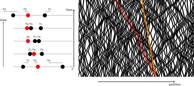
Figure 1. The simplest system that exhibits GHD is arguably the classical hard rod gas, i.e. identical billiard balls whose motion is restricted to a line. (Left) The balls collide elastically and exchange their velocities. One can re-index the balls after each collision so that the ‘bare’ velocity vj is constant (here the red ball is the one with velocity v2 at any time). (Right) At large distance and time scales, the effective velocity of the red ball veff (red trajectory) is different from its ‘bare’ velocity v (orange trajectory). The GHD description of the hard rod gas (4) is an Euler hydrodynamic limit where the interactions between the particles enter through the effective velocity.
Download figure:
Standard image High-resolution imageOne can introduce a coarse-grained phase-space density of balls  , where δℓ
and δσ
are smooth distributions with weight one peaked around the origin, for instance two Gaussians of width ℓ and σ. When ℓ and σ are large enough that the phase-space volume [x, x + ℓ] × [v, v + σ] contains a very large number of balls, but small enough that the density stays constant throughout the volume, the coarse-grained density evolves according to the two equations
, where δℓ
and δσ
are smooth distributions with weight one peaked around the origin, for instance two Gaussians of width ℓ and σ. When ℓ and σ are large enough that the phase-space volume [x, x + ℓ] × [v, v + σ] contains a very large number of balls, but small enough that the density stays constant throughout the volume, the coarse-grained density evolves according to the two equations

where we have included an external potential V(x). These are the GHD equations for the hard rod gas, initially derived by Percus (1976), and proved by Boldrighini et al (1983) for V(x) = 0. The inclusion of the trapping potential, and its breaking of the conservation laws, was investigated more recently by Cao et al (2018).
The first equation (4) is similar to the transport equation (1), although two important differences need to be stressed. The first difference lies in the range of applicability of equation (4): it is a coarse-grained description of the hard rod gas based on local relaxation, which is valid only at the Euler scale. The free transport equation (1), on the other hand, does not rely on hydrodynamic assumptions. The second difference is that, instead of the single-particle group velocity, equation (4) involves an ‘effective velocity’. That effective velocity is a functional of the density ρ(v) at a given position x and time t, defined by the second equation (4). It has a simple interpretation, see figure 1. At each collision, the labels of the colliding balls can be switched, so that each velocity vj stays constant, but the position xj changes instantaneously by ±|Δ| (the diameter of the balls). For a finite density of balls, these jumps result in a modification of the propagation velocity of the ball with velocity vj through the gas, vj → veff[ρ](vj ).
The GHD equations (4) are also analogous to the Euler hydrodynamic equations (2) and (3), but for infinitely many charges. All the charges are conserved in the absence of an external potential (V(x) = 0), while for V(x) ≠ 0 only the conservation of mass and energy are expected to survive, generically. To see this, consider the aforementioned charges ![$Q[f]={\sum }_{j=1}^{N}f\enspace ({v}_{j})$](https://content.cld.iop.org/journals/1742-5468/2022/1/014003/revision6/jstatac3659ieqn13.gif) , and their associated charge densities
, and their associated charge densities ={\int }_{-\infty }^{\infty }\;f\enspace (v)\rho (x,v,t)\mathrm{d}v$](https://content.cld.iop.org/journals/1742-5468/2022/1/014003/revision6/jstatac3659ieqn14.gif) . Those charge densities evolve according to
. Those charge densities evolve according to

When V(x) = 0, the first equation is a continuity equation that expresses the conservation of Q[f]. The second line gives the expectation value of the current as a function of the charge densities under the hydrodynamic assumptions.
Thus, as claimed above, GHD captures a peculiar fluid-like behavior which resembles both a fluid obeying the free transport equation (1), and one obeying the Euler hydrodynamic equations (2) and (3).
Remarkably, the GHD equations (4) reappeared in 2016, in the context of quantum integrable 1D systems (Bertini et al 2016, Castro-Alvaredo et al 2016). In the decade that preceded this 2016 breakthrough, tremendous progress had been made on out-of-equilibrium quantum dynamics, largely driven by advances in cold atom experiments. To name but one example, the 2006 quantum Newton cradle experiment of Kinoshita et al (2006), where two 1D clouds of interacting atoms in a harmonic potential V(x) undergo thousands of collisions, seemingly escaping convergence toward thermal equilibrium, had become an important source of inspiration and a challenge for quantum many-body theorists. Many important conceptual advances on the thermalization (or absence thereof) of isolated quantum systems, in particular developments around the notion of GGE, occurred between 2006 and 2016, and yet a quantitatively reliable modeling of the quantum Newton cradle setup, with experimentally realistic parameters, had remained completely out of reach. As usual with quantum many-body systems, the exponential growth of the Hilbert space with the number of atoms N seemingly prevented direct numerical simulations of the dynamics.
The 2016 breakthrough of GHD has completely changed this state of affairs. Realizing that the dynamics of 1D ultracold quantum gases in experiments such as the quantum Newton cradle is captured by GHD equations of the form (4) has ushered in a new era for their theoretical description.
Goal of this review and organization. Our purpose is to give a pedagogical overview of the developments that have occurred in the study of the 1D Bose gas since the 2016 discovery of GHD in quantum integrable systems (Bertini et al 2016, Castro-Alvaredo et al 2016). Because the topic is of interest to both cold atom physicists and quantum statistical physicists, we have attempted to write this review article in a way that makes it accessible to all.
The article is organized as follows. In section 1 we review the basic facts about the theory of the 1D Bose gas that are useful for understanding the development of GHD. We provide an introduction to the repulsive Lieb–Liniger model, with a strong emphasis on the key concept of the rapidities. We also review the asymptotic regimes of the 1D Bose gas (quasicondensate, ideal Bose gas, and hard-core regimes), which are often important in the description of experiments. In section 2 we present the GHD description of the 1D Bose gas, and review the theoretical results that have been obtained since 2016 with this approach. In section 3 we briefly review the experimental setups that have been used to realize 1D Bose gases, and the main experimental results obtained in connection with integrability. In that section we focus mostly on results obtained prior to the advent of GHD. Then, in section 4, we present the experimental tests of GHD, and recent experiments whose descriptions have relied on GHD. In section 5 we briefly discuss the recent theoretical developments that aim to describe the effects of atom losses. We discuss some perspectives and open questions in the conclusion.
1. The Lieb–Liniger model and the rapidities
In the absence of an external potential, the Hamiltonian of 1D bosons with delta repulsion is, in second-quantized form,

Here Ψ†(x) and Ψ(x) are the boson creation/annihilation operators that satisfy the canonical commutation relations ![$\left[{\Psi}(x),{{\Psi}}^{{\dagger}}({x}^{\prime })\right]=\delta (x-{x}^{\prime })$](https://content.cld.iop.org/journals/1742-5468/2022/1/014003/revision6/jstatac3659ieqn15.gif) , m is the mass of the bosons, g > 0 is the 1D repulsion strength, and μ is the chemical potential. The total number of particles in the system is
, m is the mass of the bosons, g > 0 is the 1D repulsion strength, and μ is the chemical potential. The total number of particles in the system is  . In the literature, it is customary to define the parameter c = mg/ℏ2, homogeneous to an inverse length. In a box of length L, the ratio of c to the particle density n = N/L gives the dimensionless repulsion strength, or Lieb parameter,

In the rest of this section we review some basic facts about the exact solution of the model (6) of Lieb and Liniger (1963); see (Gaudin 2014, Korepin et al 1997) for introductions. In particular, we emphasize the crucial concept of the rapidities, and we review a number of results that have proved useful in recent developments in GHD. We set ℏ = m = 1.
1.1. The scattering shift (or Wigner time delay)
It is instructive to start with the case of N = 2 particles on an infinite line. In first quantization, using center-of-mass and relative coordinates X = (x1 + x2)/2 and Y = x1 − x2, the Hamiltonian (6) splits into a sum of two independent one-body problems,

The eigenstates of the center-of-mass Hamiltonian  are plane waves, and the Hamiltonian for the relative coordinate Y is that of a particle of mass 1/2 in the presence of a delta potential at Y = 0. Because of that delta potential, the first derivative of the wavefunction φ(Y) must have a discontinuity at Y = 0: φ′(0+) − φ′(0−) − c φ(0) = 0. Coming back to the original coordinates, one sees that the two-body wavefunction
  satisfies

The same condition holds for x1 exchanged with x2, since the wavefunction is symmetric. Thus the eigenstates of (8) are

corresponding to the eigenvalues  . For θ1 > θ2, the two terms
  and
and  correspond to the incoming and outgoing pairs of particles in a two-body scattering process. The ratio of their amplitudes is the two-body scattering phase,

An equivalent expression for that phase, often used in the literature and which we also use below, is ϕ(θ) = 2 arctan(θ/c) ∈ [−π, π].
It was pointed out by Eisenbud (1948) and by Wigner (1955) that the scattering phase may be viewed semiclassically as a ‘time delay’. Let us briefly sketch the argument of Wigner (1955). First, we note that, for a single particle, a simple substitute for a wavepacket is a superposition of two plane waves with momenta θ and θ + δθ,

Such a superposition evolves in time as eixθ−itɛ(θ) + eix(θ+δθ)−itɛ(θ+δθ), where ɛ(θ) = θ2/2 is the energy. The center of this ‘wavepacket’ is at the position where the phases of the two terms coincide, namely the point where xδθ − t[ɛ(θ + δθ) − ɛ(θ)] = 0, which gives x ≃ vt with the group velocity v = dɛ/dθ = θ. So this is indeed a ‘wavepacket’ moving at speed θ. Next, consider two incoming particles in a state such that the center of mass (x1 + x2)/2 has momentum θ1 + θ2, while the relative coordinate x1 − x2 is in a ‘wavepacket’ moving at velocity (θ1 − θ2)/2,

According to equations (10) and (11), the corresponding outgoing state would be

Then, repeating the previous argument of phase stationarity, one finds that the relative coordinate is at position  at time t. Since the center of mass is not affected by the collision and moves at the group velocity (θ1 + θ2)/2, we see that the position of the two semiclassical particles after the collision will be

where the scattering shift Δ(θ) is given by the derivative of the scattering phase,

The two particles are delayed: their position after the collision is the same as if they were late by a time δt1 = Δ(θ2 − θ1)/v1 and δt2 = Δ(θ2 − θ1)/v2 respectively.
1.2. The Bethe wavefunction, and the rapidities as asymptotic momenta
For more particles, the eigenstates of the Hamiltonian (6) on the infinite line are Bethe states  labeled by a set of N numbers
  , called the rapidities. In the domain x1 < x2 < ⋯ < xN
, the wavefunction is (Gaudin 2014, Korepin et al
1997, Lieb and Liniger 1963)
, called the rapidities. In the domain x1 < x2 < ⋯ < xN
, the wavefunction is (Gaudin 2014, Korepin et al
1997, Lieb and Liniger 1963)

and it is extended to other domains by symmetry xi ↔ xj . Here the sum runs over all permutations σ of N elements (so there are N! terms) and (−1)|σ| is the signature of the permutation. The momentum and energy of the eigenstate (17) are

The rapidities θa are conveniently thought of as the asymptotic momenta in an N-body scattering process. For θ1 > θ2 > ⋯ > θN , the combination of two terms

that appears in (17) can be viewed as the sum of incoming ( ) and outgoing states (
 ) in an N-body scattering process, see figure 2. Their respective amplitude
  is a many-body phase, which depends on all incoming rapidities. Crucially, this many-body phase factorizes into a product of two-body scattering phases (11); this is a central property of all quantum integrable systems.
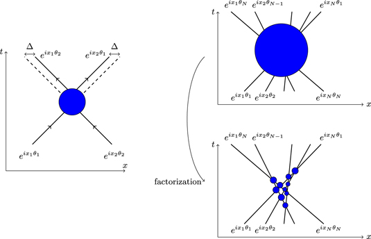
Figure 2. (Left) The wavefunction (10) on the infinite line corresponds to a two-body scattering process. Semiclassically, the scattering phase in that two-body process is reflected in the scattering shift (16): after the collision, the position of the particle has been shifted by a distance Δ(θ1 − θ2). (Right) The Bethe wavefunction (17) on the infinite line corresponds to an N-body scattering process which factorizes into two-body processes (the scattering shift Δ is also present here, but it is not drawn in the illustration). In that N-body process, the rapidities θj are the asymptotic momenta of the bosons.
Download figure:
Standard image High-resolution image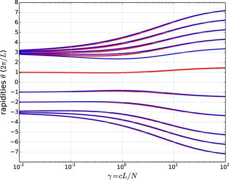
Figure 3. Blue curves: rapidities θa
obtained by solving the Bethe equations (24) with N = 10 and  , or the equivalent form (27) with
  . The rapidity θa
interpolates between
. The rapidity θa
interpolates between  (when c → 0) and pa
(c → ∞). Red curves: rapidities obtained after the modification (p5 = 3.5) → (p5 = 1.5). This shows that the rapidities are all coupled: changing only one of the pa
results in small shifts of all the other rapidities.
(when c → 0) and pa
(c → ∞). Red curves: rapidities obtained after the modification (p5 = 3.5) → (p5 = 1.5). This shows that the rapidities are all coupled: changing only one of the pa
results in small shifts of all the other rapidities.
Download figure:
Standard image High-resolution image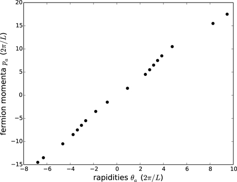
Figure 4. Fermion momenta pa
plotted against the rapidities θa
for the solution of the Bethe equations (24) defined by  with γ = 0.2. As the density of momenta pa
and of rapidities θa
increases, this becomes a smooth curve, whose slope is 2π times the density of states ρs(θ), see equation (38).
with γ = 0.2. As the density of momenta pa
and of rapidities θa
increases, this becomes a smooth curve, whose slope is 2π times the density of states ρs(θ), see equation (38).
Download figure:
Standard image High-resolution imageThe fact that the rapidities are the asymptotic momenta in a scattering process implies that they can be measured by letting the bosons expand freely along the infinite line (Bolech et al 2012, Buljan et al 2008, Campbell et al 2015, Caux et al 2019, Del Campo 2008, Jukić et al 2008, Malvania et al 2021, Mei et al 2016, Minguzzi and Gangardt 2005, Rigol and Muramatsu 2005, Wilson et al 2020). Here we follow the argument of Campbell et al (2015).
Consider a state  of N bosons confined to some interval around the origin at time t. This could be, for instance, the ground state in a trapping potential V(x), or some out-of-equilibrium state produced by some quench protocol, also in a trapping potential to ensure that the bosons are initially confined. This many-body state can be expanded on the basis of Bethe states,

where the Bethe states on the infinite line are normalized such that  (assuming that both sets of rapidities are ordered, θ1 > ⋯ > θN
and
(assuming that both sets of rapidities are ordered, θ1 > ⋯ > θN
and  ). The integral is restricted to the domain θ1 > θ2 > ⋯ > θN
in the first line to avoid double-counting. Notice that, with the definition (17), the Bethe states are anti-symmetric under exchange of two rapidities θa
↔ θb
. Then, plugging (17) into (20), and using this anti-symmetry, one obtains (Campbell et al
2015)
). The integral is restricted to the domain θ1 > θ2 > ⋯ > θN
in the first line to avoid double-counting. Notice that, with the definition (17), the Bethe states are anti-symmetric under exchange of two rapidities θa
↔ θb
. Then, plugging (17) into (20), and using this anti-symmetry, one obtains (Campbell et al
2015)

for x1 < x2 < ⋯ < xN . This expression is particularly convenient for analyzing the expansion. When the trapping potential V(x) is switched off at time t, and the bosons are left to evolve freely along the infinite line, the probability of finding them at positions x1, x2, …, xN after an expansion time texp is

From the second to the third line, we have used the stationary phase approximation, taking the limit texp → ∞ while keeping the ratios x1/texp, …, xN
/texp fixed. The proportionality factor is fixed by imposing that  .
.
In conclusion, we see from (22) that the joint probability distribution of the positions of the atoms after a large 1D expansion time directly reflects the distribution of rapidities in the state  just before the expansion. This is very important because it means that the rapidities can be measured experimentally, by performing such 1D expansions. This was done experimentally for the first time by Wilson et al (2020). This experiment is discussed in section 3 below.
1.3. Finite density and the Bethe equations
In the two previous subsections, we have focused on a finite number of bosons on an infinite line, corresponding to a vanishing density of particles. But, to understand the thermodynamic properties of the model, one needs to work with a finite density N/L. This can be done by imposing periodic boundary conditions, identifying the points x = 0 and x = L in the system. Imposing periodic boundary conditions on the Bethe wavefunction (17), i.e.  , leads to the Bethe equations

where the two-body scattering phase ϕ(θa − θb ) is defined in equation (11). Taking the logarithm on both sides, one gets the following system of N coupled non-linear equations:

It is convenient to think of the numbers pa
as the momenta of N non-interacting fermions (with periodic or anti-periodic boundary conditions, depending on the parity of N). These fermion momenta have the following interpretation: for fixed N and L, one can adiabatically follow each eigenstate  as one varies the repulsion strength c. In the infinite repulsion limit c → +∞, the bosonic wavefunction (17) is, up to multiplication by a sign ∏a<b
sign(xb
− xa
), equal to the Slater determinant of N non-interacting fermions, i.e.
as one varies the repulsion strength c. In the infinite repulsion limit c → +∞, the bosonic wavefunction (17) is, up to multiplication by a sign ∏a<b
sign(xb
− xa
), equal to the Slater determinant of N non-interacting fermions, i.e. ![$\mathrm{det}{\left[{\text{e}}^{\text{i}{x}_{a}{\theta }_{b}}\right]}_{1\leqslant a,b\leqslant N}$](https://content.cld.iop.org/journals/1742-5468/2022/1/014003/revision6/jstatac3659ieqn39.gif) (Girardeau 1960). In that limit, the rapidities are nothing but the momenta of these non-interacting fermions: θa
= pa
. Importantly, the fermions in the c → +∞ limit must obey the Pauli exclusion principle, so all momenta should be different: pa
≠ pb
if a ≠ b. In the following we order both the rapidities and the fermion momenta as
(Girardeau 1960). In that limit, the rapidities are nothing but the momenta of these non-interacting fermions: θa
= pa
. Importantly, the fermions in the c → +∞ limit must obey the Pauli exclusion principle, so all momenta should be different: pa
≠ pb
if a ≠ b. In the following we order both the rapidities and the fermion momenta as

It is natural to wonder what happens in the opposite limit of non-interacting bosons, c → 0. This is easily answered by introducing the ‘boson momenta’  , related to the fermion momenta pa
as
, related to the fermion momenta pa
as

Notice that  ; in particular, two or more boson momenta can coincide. Using the fact that
  , equation (24) is equivalent to

For c > 0, the ‘momenta’  are just another way of parameterizing the solutions of the Bethe equations; they should not be confused with the momenta of the atoms, which would be obtained by computing the momentum distribution
  , where
  is the Fourier mode of the creation operator Ψ†(x). However, in the limit of vanishing repulsion c → 0, the rapidities are nothing but the boson momenta,
  . Moreover, in that limit, the Bethe wavefunction (17) is nothing but the permanent
 ![$\mathrm{p}\mathrm{e}\mathrm{r}{[{\text{e}}^{\text{i}{x}_{a}{\theta }_{b}}]}_{1\leqslant a,b\leqslant N}$](https://content.cld.iop.org/journals/1742-5468/2022/1/014003/revision6/jstatac3659ieqn47.gif) , i.e. the wavefunction of N non-interacting bosons. So, in that limit, the rapidities coincide with the atom momenta.
, i.e. the wavefunction of N non-interacting bosons. So, in that limit, the rapidities coincide with the atom momenta.
Away from these two limits, the rapidities θa correspond to an adiabatic interpolation between the non-interacting fermion (c → +∞) and boson (c → 0) momenta, obtained by solving the Bethe equations (24), see figure 3.
In general, the Bethe equations (24) cannot be solved analytically, but they can easily be solved numerically. One efficient way of doing this is to use the Newton–Raphson method.
1.4. Conserved charges and currents
The eigenstates of the Lieb–Liniger Hamiltonian (6) are Bethe states  labeled by their sets of rapidities. This allows us to define a family of charge operators Q[f], diagonal in the eigenbasis and parameterized by functions
  , such that

Both the momentum operator and the Hamiltonian are of that form, with f(θ) = θ and f(θ) = θ2/2 respectively, see equation (18). It is the integrability of the model, reflected in the structure of the eigenstates (17), which allows us to consider the more general conserved charges (28). By construction, all these operators commute: [Q[f1], Q[f2]] = 0. In general, an explicit expression for Q[f] in second-quantized form (like Q[θ2/2] given by equation (6)) is not known, and typically regularization issues appear when one tries to write it (Davies 1990). Nevertheless, even in the absence of such direct expressions for the charges, the conserved charges Q[f] defined formally by equation (28) prove to be very useful. There are other ways to perform calculations with these charges, that do not require one to know their explicit second-quantized form, in particular the algebraic Bethe ansatz, see e.g. (Korepin et al 1997) for an introduction.
From their definition (28), one expects the Q[f] charges to be extensive with N, and to be the integral of a charge density

For f sufficiently regular, the charge density q[f](x) is sufficiently local, meaning that it vanishes quickly away from the point x. (In the hard-core limit g → +∞, this is a consequence of the Paley–Wiener theorem. At finite repulsion strength g, and more generally in interacting integrable models, the locality properties of charge densities are an advanced topic that is beyond the scope of this review, see e.g. (Doyon 2017, Ilievski et al
2016, Palmai and Konik 2018) for introductions.) By definition, the expectation value of the charge density in a Bethe state (normalized as  ) is
) is

It is independent of x because the Bethe state is translation invariant.
To the charge density q[f], one associates a current operator j[f] through the continuity equation,

As sketched in the introduction, continuity equations are the basic ingredient of hydrodynamics. To write useful hydrodynamic equations, however, one must be able to evaluate the currents in given stationary states. Until very recently, it was not known how to evaluate the expectation values of the current j[f]. However, thanks to developments in integrability, in particular in form factor techniques and the algebraic Bethe ansatz, a remarkable exact formula has just been discovered by Borsi et al (2020) for the expectation value of j[f] in a Bethe state (see also (Pozsgay 2020a, 2020b) for further developments in the context of spin chains, as well as the review article by Borsi et al (2021) in this volume),

Here ɛ′(θ) = θ is the derivative of ɛ(θ) = θ2/2, and  is the Jacobian matrix of the transformation from the pa
to the θb
defined by equation (24), known as the Gaudin matrix,
is the Jacobian matrix of the transformation from the pa
to the θb
defined by equation (24), known as the Gaudin matrix,

(where the pa
in equation (24) are no longer restricted to be in  ). The Gaudin matrix is symmetric,
  , as a consequence of the fact that the scattering phase ϕ depends on the rapidities θa
and θb
only through the difference θa
− θb
, see equation (16).
, as a consequence of the fact that the scattering phase ϕ depends on the rapidities θa
and θb
only through the difference θa
− θb
, see equation (16).
Let us mention that the remarkable formula (33) is a particular case of a more general result, also obtained in (Borsi et al 2020, Pozsgay 2020a, 2020b). One can define generalized currents j[h, f](x) through the generalization of the continuity equation (31):

Then the general formula for the expectation value reads

and the above physical current is the special case h(θ) = ɛ(θ) = θ2/2. We note that such generalized currents had also been considered in (Castro-Alvaredo et al 2016) in the thermodynamic limit.
The discovery and proof of formula (34) or its generalization (35) required advanced techniques (Borsi et al
2020, Pozsgay 2020a, 2020b), however the result is simple and its physical interpretation is quite clear. The bth boson, with rapidity θb
, carries an amount of charge density  . In the absence of other particles, it would travel at the single-particle group velocity vb
= ∂ɛ(θb
)/∂p(θb
) = ∂ɛ(θb
)/∂θb
(or its generalization
. In the absence of other particles, it would travel at the single-particle group velocity vb
= ∂ɛ(θb
)/∂p(θb
) = ∂ɛ(θb
)/∂θb
(or its generalization  , resulting in the current
 ![$j[h,f]=\frac{1}{L}{v}_{b}f\enspace ({\theta }_{b})$](https://content.cld.iop.org/journals/1742-5468/2022/1/014003/revision6/jstatac3659ieqn56.gif) .
.
In the presence of other particles, the group velocity of the bth boson is modified. To compute it, one can consider a small variation of the fermion momentum pb
→ pb
+ δpb
in equation (24). This results in a small change of the total momentum δP = δpb
, and of the total energy ![$\delta E=\delta \left({\sum }_{a=1}^{N}\varepsilon ({\theta }_{a})\right)={\sum }_{a}\frac{\partial \varepsilon ({\theta }_{a})}{\partial {p}_{b}}\delta {p}_{b}={\sum }_{a}\;{\varepsilon }^{\prime }({\theta }_{a}){[{\mathcal{G}}^{-1}]}_{ab}\delta {p}_{b}$](https://content.cld.iop.org/journals/1742-5468/2022/1/014003/revision6/jstatac3659ieqn57.gif) (more generally, of the total charge
(more generally, of the total charge ![$\delta Q[h]={\sum }_{a}\frac{\partial h({\theta }_{a})}{\partial {p}_{b}}\delta {p}_{b}={\sum }_{a}{h}^{\prime }({\theta }_{a}){[{\mathcal{G}}^{-1}]}_{ab}\delta {p}_{b}\left. \right)$](https://content.cld.iop.org/journals/1742-5468/2022/1/014003/revision6/jstatac3659ieqn58.gif) ). Thus, the modified group velocity is
). Thus, the modified group velocity is ![$\delta E/\delta {p}_{b}={\sum }_{a}\;{\varepsilon }^{\prime }({\theta }_{a}){[{\mathcal{G}}^{-1}]}_{ab}$](https://content.cld.iop.org/journals/1742-5468/2022/1/014003/revision6/jstatac3659ieqn59.gif) , resulting in formula (32), or more generally
, resulting in formula (32), or more generally ![$\delta Q[h]/\delta {p}_{b}={\sum }_{a}\;{h}^{\prime }({\theta }_{a}){[{\mathcal{G}}^{-1}]}_{ab}$](https://content.cld.iop.org/journals/1742-5468/2022/1/014003/revision6/jstatac3659ieqn60.gif) , resulting in (35).
, resulting in (35).
For further discussions of the physical interpretation of equations (32) and (35), see (Borsi et al 2020) and also (Bertini et al 2016, Bonnes et al 2014, Castro-Alvaredo et al 2016, Doyon 2019b, Doyon et al 2018), where similar discussions had been presented previously for the thermodynamic version of these formulas (see equation (46) below). See also the two reviews by Borsi et al (2021) and by Cubero et al (2021) in this volume.
1.5. Thermodynamic limit
So far we have focused on a finite number of bosons N, first on an infinite line, and then in a periodic box of length L. For hydrodynamics, one needs first to understand the thermodynamic properties of the system. In this subsection, we briefly review the techniques for taking the thermodynamic limit N, L → ∞, keeping the density of bosons n = N/L fixed.
The key idea is to focus on an infinite sequence of eigenstates  of the Lieb–Liniger Hamiltonian (6), with L = N/n, such that the limit of the distribution of rapidities

is well defined and is a (piecewise) smooth function of θ. The thermodynamic properties of the system (such as its energy density, pressure, etc) then become particular functionals of that rapidity density ρ(θ), and the goal is to find these functionals and to evaluate them. In what follows, we write ‘limtherm.’ for this limiting procedure.
For example, consider the expectation values of the charge densities (30): in the thermodynamic limit, these become

In particular, the density of particles, the momentum density and the energy density are, respectively, ![$n=\left\langle q[1]\right\rangle =\int \rho (\theta )\mathrm{d}\theta $](https://content.cld.iop.org/journals/1742-5468/2022/1/014003/revision6/jstatac3659ieqn62.gif) ,
, ![$\left\langle q[\theta ]\right\rangle =\int \theta \rho (\theta )\mathrm{d}\theta $](https://content.cld.iop.org/journals/1742-5468/2022/1/014003/revision6/jstatac3659ieqn63.gif) and
and ![$\left\langle q[{\theta }^{2}/2]\right\rangle =\int \frac{{\theta }^{2}}{2}\rho (\theta )\mathrm{d}\theta $](https://content.cld.iop.org/journals/1742-5468/2022/1/014003/revision6/jstatac3659ieqn64.gif) .
.
1.5.1. Thermodynamic form of the Bethe equations
Crucially, since all the states in the infinite sequence  are Bethe states, each set of rapidities
  must satisfy the Bethe equations (24). To implement that constraint, it is customary to consider the set of fermion momenta
  associated to the set of rapidities
  , both of them ordered as in (25), and to define the density of states ρs(θ) as (see figure 4)

where the sequence of indices a in the rhs is chosen so that limtherm.
θa
= θ. Because the fermion momenta pa
must satisfy the Pauli exclusion principle (they must all be different), it is clear that  . Also, notice that, by definition,
  . Consequently, the Fermi occupation ratio

must always satisfy

Moreover, the rapidity density ρ(θ) and the density of states ρs(θ) are related by the thermodynamic version of the Bethe equation (24). Plugging equation (24) into the definition (38) leads to the constitutive equation
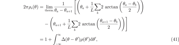
where Δ(θ − θ′) is the differential two-body scattering shift (16).
In practice, to construct interesting thermodynamic states, one can specify the Fermi occupation ratio ν(θ), and then use the constitutive equation (41) to reconstruct the rapidity density ρ(θ) and the density of states ρs(θ). One important example of this is the ground state of the Lieb–Liniger Hamiltonian, which corresponds to an occupation ratio which is a rectangular function: ν(θ) = 1 for θ ∈ [−θF, θF], and ν(θ) = 0 otherwise. Here θF is the Fermi rapidity, which is a function of the density of particles n. In that case, the constitutive equation becomes the Lieb equation (Lieb and Liniger 1963) (also known as the Love equation (Love 1949); for studies of this particular equation see e.g. (Lang et al 2017, Mariño and Reis 2019, Popov 1977, Prolhac 2017, Takahashi 1975). Another important example is that of a thermal equilibrium distribution ρ(θ) obtained by solving the Yang–Yang equation (equation (57) below).
In general, the constitutive equation cannot be solved analytically, however, since it is linear, it is easily solved numerically by discretizing the integral.
1.5.2. The dressing
In thermodynamic manipulations, it turns out that the following operation is ubiquitous: to a function f(θ), one has to associate its ‘dressed’ counterpart fdr(θ), defined by the integral equation

Although it is not explicit in the notation, fdr(θ) is always a functional of the rapidity distribution, through its dependence on the Fermi occupation ratio. For instance, with this definition, the constitutive equation (41) is recast as

where 1(θ) = 1 is the constant function.
Another example where the dressing (42) pops out is in manipulations that involve the Gaudin matrix. This is important for this review article, because to establish hydrodynamic equations one needs the thermodynamic limit of the expectation value of the current, see equation (32). The following identity holds:

where, again, the relation between θ in the lhs and the rapidity θa in the rhs is θ = limtherm. θa . This identity is easily derived as follows. Using the definition (33),
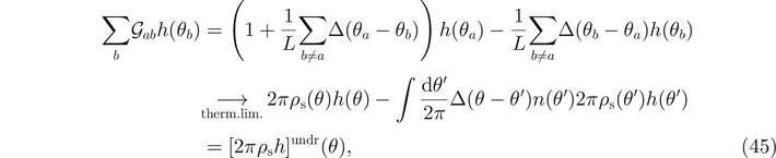
where the ‘undressing’ is the inverse of the dressing, i.e.  . Inverting this formula gives equation (44).
We will see a few more examples of physical quantities whose computation involves the dressing operation below. References where this operation is used extensively include, for example, the original derivation of the GHD equations in integrable quantum field theories (Castro-Alvaredo et al 2016), the calculation of Drude weights and other two-point correlations of charge and currents in the Lieb–Liniger model (Doyon and Spohn 2017a) and the inclusion of force fields (Doyon and Yoshimura 2017), adiabatically varying interactions (Bastianello et al 2019) or diffusive corrections (De Nardis et al 2018, 2019, Gopalakrishnan et al 2018) into the GHD equations.
1.5.3. Expectation values of the currents in the thermodynamic limit
We now present the central ingredient of GHD. The thermodynamic expectation value of the current j[f] (see subsection 1.4) is

where the effective velocity is a functional of the rapidity distribution defined by

with ɛ′(θ) = id(θ) = θ and 1(θ) = 1. The remarkable result (46) was first obtained by Bertini et al (2016), Castro-Alvaredo et al (2016), and it was the key observation that triggered all the later developments of GHD in quantum integrable systems. Bertini et al (2016) relied partially on (Bonnes et al 2014), where the formula for the effective velocity (47) had first appeared in the context of a quantum integrable system. In retrospect, the thermodynamic result (46) can be viewed as a consequence of the finite-size formula (32) of Borsi et al (2020), Pozsgay (2020a, 2020b), using the fact that the dressing is the thermodynamic limit of the Gaudin matrix, see equation (44). Historically though, the thermodynamic result was discovered before its finite-size counterpart. Since 2016, several works have aimed to establish the validity of the thermodynamic formula (46) in various models, by relying on various approaches. Let us mention the form factor approaches of Cubero (2020), Cubero and Panfil (2020), Vu and Yoshimura (2019) for quantum field theories, and arguments based on the symmetry of the charge–current correlations (Yoshimura and Spohn 2020) or exact results in the classical integrable model of the Toda chain (Bulchandani et al 2019, Cao et al 2019, Doyon 2019a, Spohn 2020). We also refer to the two reviews on this topic by Cubero et al (2021) and by Borsi et al (2021) in this volume.
The effective velocity (47) solves the equation

This is analogous to equation (4) in the introduction, which defines the effective velocity in the hard rod gas. The main difference is that the scattering shift Δ(θ − θ′) is now rapidity-dependent, while in the hard rod gas Δ is a constant equal to minus the diameter of the balls. The physical interpretation of equation (48) is analogous to that shown in figure 1: a ‘tracer’ quasiparticle with rapidity (asymptotic momentum) θ, which would normally travel at constant speed θ in a vacuum, finds its velocity modified by the presence of a finite density ρ(θ′) of other quasiparticles. From time t to t + δt, the tracer typically scatters against a number δt × |veff[ρ](θ) − veff[ρ](θ′)|ρ(θ′) of quasiparticles with rapidity θ′. At each collision, the tracer is shifted backwards by an amount Δ(θ − θ′): this is the physical effect that is encoded by formula (48).
To check that the effective velocity (47) solves equation (48) as claimed, one can use the definition of the dressing and the constitutive relation:
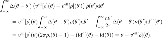
1.6. Entropy maximization: the Yang–Yang equation
In the previous subsection we illustrated how physical observables, such as the expectation values of charges and currents, become functionals of the rapidity distribution ρ(θ) in the thermodynamic limit. We did not explain how to construct physically meaningful rapidity distributions though (except for the ground state of the Lieb–Liniger Hamiltonian, for which ν(θ) is a rectangular function, see subsection 1.5).
For instance, what is the rapidity distribution corresponding to a thermal equilibrium state at non-zero temperature? This question was answered in the pioneering work of Yang and Yang (1969), which we now briefly review.
First, we observe that there are many different choices of sequences of eigenstates  that lead to the same thermodynamic rapidity distribution (36). The description of the system in terms of a rapidity distribution ρ(θ) is only a coarse-grained description: one should think of the rapidity distribution ρ(θ) as characterizing a macrostate of the system, corresponding to a very large number of possible microstates
  . For thermodynamics, one needs to estimate the number of such microstates.
To estimate that number, one focuses on a small rapidity cell [θ, θ + δθ], which contains Lρ(θ)δθ rapidities. The Bethe equations (24) relate these rapidities to fermion momenta pa
in a momentum cell [p, p + δp], where δp/δθ ≃ 2πρs(θ), see equation (38). Importantly, the fermion momenta pa
satisfy the Pauli exclusion principle. Then the number of microstates is evaluated by counting how many configurations of mutually distinct Lρ(θ)δθ fermion momenta can fit into the box [p, p + δp]. Since the minimal spacing between two momenta is  , the answer is

The total number of microstates is the product of all such configurations over all the rapidity cells [θ, θ + δθ]. Taking the logarithm, and replacing the sum by an integral over dθ, we obtain the Yang–Yang entropy

The notation indicates that the Yang–Yang entropy is a functional of ρ only, and not of ρs; this is because ρs must always be obtained from ρ by the constitutive equation (41).
Now let us consider the thermal equilibrium density matrix at temperature T,

where the sum runs over all eigenstates. In fact, a straightforward generalization consists of considering the GGE (Rigol et al 2008, 2007) density matrix

for some function f. We would like to compute expectation values w.r.t. this density matrix, for example

for some observable  . When the observable
  is sufficiently local, it is believed that the expectation value
  does not depend on the specific microstate of the system, so that it becomes a functional of ρ in the thermodynamic limit,

This assumption is related to a ‘generalized eigenstate thermalization hypothesis’, see e.g. (Cassidy et al 2011, Dymarsky and Pavlenko 2019, He et al 2013, Pozsgay 2011, 2014, Vidmar and Rigol 2016). Under that assumption, one can replace the above sum over all eigenstates by a functional integral over the coarse-grained rapidity distribution ρ,

The functional integral is then dominated by the root distribution which minimizes a (generalized) free energy functional:

Using the definition of the Yang–Yang entropy and the constitutive equation (24), one obtains the following relation between the function f(θ) defining the diagonal density matrix (52) and the rapidity distribution ρ(θ) dominating the functional integral (55):

This equation is known as the (generalized) Yang–Yang equation, or (generalized) thermodynamic Bethe ansatz equation. Again, the term ‘generalized’ refers to the replacement of the thermal equilibrium density matrix by a GGE, (51) → (52), see e.g. (Caux and Konik 2012, Wouters et al 2014). Like most of the equations encountered so far, in general the Yang–Yang equation cannot be solved analytically, but it can be efficiently solved numerically, by iteration. In particular, this allows us to compute the rapidity distribution ρ(θ) at thermal equilibrium.
This is particularly useful in applications discussed later in this review, because in experiments one often assumes that the system is (at least initially) at thermal equilibrium.
For instance, using the Yang–Yang equation, it is possible to tabulate the equilibrium pressure  as a function of the particle density n and the energy per particle e. To do this, one needs to first solve numerically equation (57) with f(θ) = (ɛ(θ) − μ)/T, and equation (41), to get ρ(θ) and ρs(θ). Then the equilibrium pressure is given by (Korepin et al
1997, Yang and Yang 1969)
as a function of the particle density n and the energy per particle e. To do this, one needs to first solve numerically equation (57) with f(θ) = (ɛ(θ) − μ)/T, and equation (41), to get ρ(θ) and ρs(θ). Then the equilibrium pressure is given by (Korepin et al
1997, Yang and Yang 1969)

where the free energy is F/L = ∫(ɛ(θ) − μ)ρ(θ)dθ − TSYY[ρ]. This gives the thermodynamic equilibrium pressure at density n = ∫ρ(θ)dθ and energy per particle  . Alternatively, the pressure can be identified with the momentum current jP
= j[id] (with id(θ) = θ) as we did in the introduction, see equation (3). Thus, according to equation (46), we must also have
. Alternatively, the pressure can be identified with the momentum current jP
= j[id] (with id(θ) = θ) as we did in the introduction, see equation (3). Thus, according to equation (46), we must also have

The equivalence between the two formulas (58) and (59) follows from manipulations of the dressing operation (42), which we leave as an exercise to the interested reader. (Hint: with the definition of the effective velocity, formula (59) is equivalent to  , while differentiating (57) w.r.t. θ and using the definition of the dressing operation leads to
  .)
.)
1.7. Relaxation in the Lieb–Liniger model
It is not a priori clear whether GGEs are relevant in the context of an isolated Lieb–Liniger gas. This question is linked to the notion of relaxation in isolated many-body quantum systems, which has been at the heart of many studies in recent decades (Polkovnikov et al 2011).
It is now well established that GGEs are relevant to describing locally an isolated Lieb–Liniger gas after relaxation, see for instance the review articles (Caux 2016, Essler and Fagotti 2016, Vidmar and Rigol 2016).
Since this point is essential in GHD theory, we briefly recall the underlying physics. Let us consider a Lieb–Liniger gas, confined in a box-like potential, and let us assume it is initially in an out-of-equilibrium state that is a pure quantum state. This quantum state expands onto many Bethe ansatz eigenstates:

Typically, the rapidity distributions of the Bethe ansatz states involved in this expansion gather around a given averaged rapidity distribution. During the time evolution, the different Bethe ansatz states, each of which evolves with its own energy, will dephase. Because of this dephasing, the contribution of cross terms will vanish at long times when computing the mean value of an observable. Thus, the mean values of the observable will undergo a relaxation and take the asymptotic value

We then invoke the generalized eigenstate thermalization hypothesis which states that expectation values of a local observable do not depend on the specific Bethe ansatz state, but are a smooth functional of the rapidity distribution. Thus, expectation values of local observables are identical for all diagonal ensembles, provided they are peaked around a given rapidity distribution. One can choose the GGE corresponding to the correct rapidity distribution, as was done in equation (54). One then finds that

To compute local observables after relaxation, one can represent the whole isolated system of length L by any diagonal ensemble peaked around the correct rapidity distribution, and the GGE plays a special role in describing a subsystem of length l. If l is both much smaller than L and much larger than microscopic correlation lengths, then the subsystem is correctly described by a GGE, the GGE accounting properly for the fluctuations in the subsystem. This property was used when analyzing local fluctuation measurements (Armijo et al 2010, Jacqmin et al 2011). The physical picture supporting the relevance of the GGE to describe the small system is that the large system acts as a reservoir of rapidities for the subsystem.
In order to show that the GGE indeed describes a system in contact with reservoirs of rapidities, we propose the following picture. Let us first discretize the rapidity space: we split it into intervals [θi , θi + δθ], where i ∈ Z, θi = iδθ and δθ is much smaller than the scale of variation of ρ. We assume now that the system is, for each integer i, in contact with a reservoir of rapidities lying in the interval [θi , θi + δθ], and we label the reservoir with the integer i. Then, statistical mechanics tells us that the density matrix of the system is

where Ni is the number of rapidities of the state |{θa }⟩ lying in the interval [θi , θi + δθ], and fi is the temperature parameter associated to the reservoir number i. Equation (63) is nothing other than the GGE ensemble given in equation (52), with a discretized function f: in each segment [θi , θi + δθ], f takes the constant value fi .
1.8. Asymptotic regimes of the Lieb–Liniger gas and approximate descriptions
So far we have seen that the thermodynamics of the Lieb–Liniger model is determined by the rapidity distribution ρ(θ), which parameterizes an infinite family of stationary states. This is in contrast with generic chaotic Galilean invariant gases, where the thermodynamic properties would depend only on the atomic density, the momentum density and the energy density. Despite the infinite-dimensional parameter space of stationary states, the Lieb–Liniger gas possesses a small number of asymptotic regimes where its description simplifies.
In this subsection, we review the three main asymptotic regimes of the Lieb–Liniger gas: the ideal Bose gas, the quasicondensate and the hard-core regimes. These three regimes arise when one compares the typical energy per atom e to two energy scales: the scattering energy mg2/ℏ2 and the mean-field interaction energy gn (where n is the atom density):
- e ≫ mg2/ℏ2, gn: ideal Bose gas regime
- e ≃ gn ≫ mg2/ℏ2: quasicondensate regime
- mg2/ℏ2 ≫ e: hard-core regime.
In the following, we discuss the phenomenology of these three regimes.
1.8.1. Ideal Bose gas regime
When e ≫ mg2/ℏ2, gn, the interactions are negligible, and the gas behaves like a gas of non-interacting bosons. The rapidity distribution coincides with the momentum distribution of the bosons, as discussed after equation (27). Alternatively, this can also be understood as a consequence of the fact that the momentum distribution of the ideal gas is preserved during a 1D expansion, and the fact that the rapidities are the asymptotic momenta after such an expansion, see subsection 1.2.
The GGE that describes the local properties of the gas takes the form of a Gaussian density matrix,  , for some function h(p). Here Ψp
= ∫e−ipx
Ψ(x)dx is the Fourier mode of the boson annihilation operator Ψ(x). One of the consequences of that general Gaussian form is that, because of Wick’s theorem, the two-body zero-distance correlation
, for some function h(p). Here Ψp
= ∫e−ipx
Ψ(x)dx is the Fourier mode of the boson annihilation operator Ψ(x). One of the consequences of that general Gaussian form is that, because of Wick’s theorem, the two-body zero-distance correlation

Thus, the gas exhibits the bosonic bunching phenomenon: whenever a boson is found inside a small interval [x, x + dx], the probability of finding another boson in that same interval is enhanced (i.e. it is larger than n dx).
We stress that the ideal Bose gas regime is not restricted to the classical, or non-degenerate, limit. The population of some bosonic modes can be highly occupied, and thus the ideal Bose gas can be highly degenerate.
This is exemplified by the case of thermal equilibrium at temperature T and chemical potential μ, with μ < 0 for the ideal Bose gas. The distribution of bosons is given by the Bose–Einstein distribution  , and there is a crossover between the classical gas (which corresponds to |μ| ≫ kB
T) and the degenerate ideal gas (|μ| ≪ kB
T). In the degenerate regime, for momenta
, and there is a crossover between the classical gas (which corresponds to |μ| ≫ kB
T) and the degenerate ideal gas (|μ| ≪ kB
T). In the degenerate regime, for momenta  , the momentum distribution is close to a Lorentzian of half-width at half-maximum
  . The atom density is then
  , so we can estimate that the gas is degenerate as long as
  , or, equivalently, as long as

On the other hand, the typical energy per particle is e ≃ |μ|. The above condition e ≫ gn, which ensures that the gas, although it is degenerate, is in the ideal Bose gas regime as opposed to the quasicondensate regime, then reads

As long as both conditions (65) and (66) are fulfilled, the thermal equilibrium gas is not in the quasicondensate regime, even though it is highly degenerate. We note that the condition (66) was first established by Kheruntsyan et al (2003), who estimated the effects of interactions on g(2)(0) perturbatively, and required that they remain small.
1.8.2. The quasicondensate regime
This regime is reached when 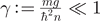 and the typical energy per atom e stays close to its value in the ground state, e ≃ gn/2. It is characterized by very small density fluctuations, with

Correlations are weak in this regime: the probability of finding an atom in a small interval [x, x + dx] is barely affected by the presence of another atom in this interval.
A good description of the gas in that regime is provided by Bogoliubov theory, or more precisely the extension of Bogoliubov theory to quasicondensates (Mora and Castin 2003). This approach assumes a phase-density representation of the bosonic field: one writes the atomic field Ψ(x) as  where ϕ and δn are the phase and density fluctuation fields, which fulfill [δn(x), ϕ(x′)] = iδ(x − x′). This approach is a coarse-grained approximation, valid for length scales much larger than the interparticle distance. The Bogoliubov approximation assumes small density fluctuations, δn(x) ≪ n, and small phase gradient, ∂ϕ(x)/∂x ≪ n. Inserting this phase–density representation into the Hamiltonian (6), one finds to second order:

This quadratic Hamiltonian allows us to determine the quantum fluctuations around the classical profile, which solves the Gross–Pitaevskii equation, i.e. n = N/L = μ/g where μ > 0 is the chemical potential. It is easily diagonalized by a Bogoliubov transformation. Defining the bosonic mode  such that [B(x), B†(x′)] = δ(x − x′), and its Fourier transform
  with
with  , one finds that the quadratic Hamiltonian becomes, up to a constant term,

where we have used μ = gn. Then the Bogoliubov transformation

with  and
and  , where
  , gives

with a dispersion relation 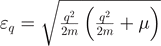 .
.
The Bogoliubov model (70) is obviously an integrable model, since it amounts to a collection of independent harmonic modes, and its integrals of motion are the population in each mode. Making the link between the Bogoliubov modes and the rapidities in the Bethe ansatz solution of the Hamiltonian (6) is, however, a difficult task. In his seminal work, Lieb (1963) described this link for states close to the ground state. He identified the so-called ‘Lieb-I excitation’ (or ‘particle excitation’) branch to the Bogoliubov modes. In a more recent investigation, Ristivojevic (2014) found that this holds in fact only for large enough momenta. Thus, to our knowledge, making the connection between rapidities and Bogoliubov modes precise remains an open problem. The difficulty of this problem is related to the difficulty of developing schemes for expansions of the thermodynamic form of the Bethe equations (41) at small γ, see e.g. (Lang et al 2017, Mariño and Reis 2019, Popov 1977, Prolhac 2017, Takahashi 1975).
1.8.3. Hard-core regime
The hard-core regime is reached when the scattering energy mg2/ℏ2 is much larger than all other intensive energy scales in the system. This is equivalent to taking g → +∞. Then, in all two-body scattering processes, the scattering phase factor (11) is one, and the scattering shift (16) vanishes. In that regime, two atoms can never be at the same position, which results in

In that regime, when a boson is found in a small interval [x, x + dx], then the probability of finding another one in the same interval is zero. This property reflects the Pauli principle satisfied by non-interacting fermions, which are related to the hard-core bosons by the non-local transformation

This transformation, closely related to the Jordan–Wigner transformation between lattice hard-core bosons and spin chains of spin-1/2, is defined such that the fermion creation/annihilation operators satisfy the canonical anticommutation relation  . In terms of these fermions, the Lieb–Liniger Hamiltonian (6) with g → +∞ becomes

This is the Hamiltonian of a non-interacting Fermi gas. The identification of hard-core bosons with non-interacting fermions remains valid in the presence of an external potential V(x).
The Bethe wavefunction is, up to a sign ∏a<b
sign(xb
− xa
), the Slater determinant of N non-interacting fermions (Girardeau 1960), and the rapidities are simply the momenta of the underlying non-interacting fermions, as discussed below equation (24). The GGEs, which describe relaxed states and which are characterized by the rapidity distribution, correspond, for the fermionic gas, to GGE states that are obtained as a product of the Gaussian density matrix for each momentum state,  , where
  is the Fourier mode of the fermion creation operator defined equation (72). (To be more precise, for finite L the fermions obey either periodic or anti-periodic boundary conditions depending on the parity of the particle number N, so the GGE is rather of the form
  , where PN even and PN odd are projectors onto the even and odd sectors. This complication can usually be omitted when one is interested in expectation values of local observables. For an example where it cannot be omitted, see e.g. (Bouchoule et al
2020) where the change of boundary conditions plays a key role in determining the effect of particle losses on the resulting GGE.)
, where PN even and PN odd are projectors onto the even and odd sectors. This complication can usually be omitted when one is interested in expectation values of local observables. For an example where it cannot be omitted, see e.g. (Bouchoule et al
2020) where the change of boundary conditions plays a key role in determining the effect of particle losses on the resulting GGE.)
The number of works that have exploited the mapping from hard-core bosons to non-interacting fermions is too large to allow us to review them all here. We simply mention a few such works that are representative in that they illustrate the typical calculations that can be done in that regime. For instance, early studies of the momentum distribution (Lenard 1964, Vaidya and Tracy 1979) revealed the presence of algebraically decaying ground state correlations, as well as the presence of tails in the momentum distribution of the atoms decaying as 1/p4 (Minguzzi et al 2002, Rigol and Muramatsu 2004). As is often the case with the 1D Bose gas, these observations remain valid beyond the hard-core regime, see e.g. the review articles (Cazalilla 2004, Cazalilla et al 2011) for long-range correlations, or (Olshanii and Dunjko 2003) about the tails of the momentum distribution. Many advances have been made in out-of-equilibrium quantum dynamics thanks to the study of the hard-core limit, for instance the early works on GGEs (Rigol et al 2007) or, more recently, investigations of trap releases (Collura et al 2013a, 2013b) and equilibration toward a GGE, or Floquet dynamics in harmonic traps (Scopa and Karevski 2017, Scopa et al 2018). For more references on hard-core bosons, we refer the reader to the bibliographies of these papers.
1.8.4. The thermal equilibrium phase diagram
In general, because of its integrability, an isolated Lieb–Liniger gas has no reason to be described by a thermal equilibrium state. Even after relaxation, the system is expected to be described by a GGE parameterized by a whole function (the rapidity distribution, see subsections 1.6 and 1.7), rather than by a Gibbs ensemble parameterized by only two parameters: the atom density n and the energy density e. However, in experiments, weak perturbations violate integrability, for instance the presence of transversely excited states (Li et al 2020, Mazets et al 2008) or the longitudinal potential (Bastianello et al 2020a). The Lieb–Liniger GGE will then be observable on an intermediate time scale, long compared to the relaxation time of the Lieb–Liniger model, but short enough that the effect of integrability breaking perturbations is still negligible. The system on this intermediate time scale is called prethermalized (Berges 2004). At very long times, the integrability breaking mechanisms will induce relaxation toward a thermal equilibrium state. Here we discuss the thermal equilibrium behavior of the 1D Bose gas, following Gangardt and Shlyapnikov (2003a), Petrov et al (2000) and especially Kheruntsyan et al (2003).
Assuming that the homogeneous 1D Bose gas is at thermal equilibrium, its state is characterized by only two dimensionless parameters: the dimensionless interaction strength γ, and the dimensionless temperature t (not to be confused with time in this subsection)

To identify the different asymptotic regimes discussed above in the phase diagram (γ, t), one can rely on the fact that g(2)(0) allows one to distinguish between them (Kheruntsyan et al 2003), see equations (64), (67) and (71). One can compute g(2)(0) using the Hellmann–Feynman theorem,

where F is the free energy per unit length, which can be computed using Yang–Yang thermodynamics (Yang and Yang 1969), see subsection 1.6. As imposed by the Hohenberg–Mermin–Wagner theorem, there is no phase transition, however the three aforementioned asymptotic regimes appear in the phase diagram, separated by smooth crossovers, see figure 5.
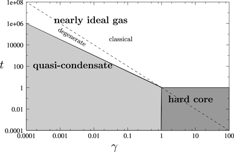
Figure 5. Phase diagram of the Lieb–Liniger model at thermal equilibrium. Different asymptotic regimes are separated by smooth crossovers. The crossover between the ideal Bose gas regime and the quasicondensate regime occurs for t ≃ γ−3/2, the crossover between the quasicondensate regime and the hard-core regime occurs for γ ≃ 1 and the crossover between the hard-core regime and the ideal Bose gas regime occurs for t ≃ 1. The dashed line represents the quantum degeneracy condition, which follows t ≃ γ−2. Note that thermal equilibrium is not granted for the Lieb–Liniger model, because of its integrability.
Download figure:
Standard image High-resolution imageIn figure 5, we represent the crossover between the ideal Bose gas regime and the quasicondensate regime, t ≃ γ−3/2, see the condition (66). The dashed line is the quantum degeneracy condition t ≃ γ−2, see (65). Above this line, the occupation numbers of single-particle quantum states are small: quantum effects are small and the gas behaves mainly as a classical gas. Below this line, the behavior depends on the regime. In the ideal Bose gas regime, low-energy single-particle states get highly populated. In the hard-core regime, the rapidity distribution, which corresponds to the momentum distribution of the equivalent Fermi gas, becomes close to that of a zero-temperature Fermi sea, namely a rectangular function.
1.8.5. The classical field approximation
We conclude this survey of the regimes of the Lieb–Liniger model by discussing the classical field approach, which, owing to its simplicity and its relevance to the description of the crossover between the quasicondensate and the degenerate ideal Bose gas, is a popular technique. In this approach, the quantization of the atomic field, i.e. the discrete nature of atoms, is ignored, and the physics boils down to that of a classical complex field ψ(x). The energy functional of this field is

and the Lagrangian is L = (iℏ/2)∫dx(ψ*∂ψ/∂t − ∂ψ*/∂tψ) − E[ψ], such that the time evolution of ψ is given by the Gross–Pitaevskii equation

The effect of an external potential is easily taken into account within this approach, by adding a term ∫dx V(x)|ψ|2 (or V(x)ψ x) to the energy functional (or to the Gross–Pitaevskii equation). This approach is expected to be meaningful in the degenerate ideal Bose gas regime, as well as in the high temperature quasicondensate regime, where the population of the modes is high. In particular, it captures the crossover between the ideal Bose gas regime and the quasicondensate regime. This approach has been used, at thermal equilibrium, to compute correlation functions (Bouchoule et al 2012, Castin 2004, Castin et al 2000, Jacqmin et al 2012) and full counting statistics (Arzamasovs and Gangardt 2019), and to investigate non-equilibrium dynamics (Bouchoule et al 2016, Thomas et al 2021). In the absence of an external potential, the Gross–Pitaevskii equation is the non-linear Schrödinger equation, a classical integrable model. The link between the classical integrals of motion and the rapidity distribution of the quantum model has been discussed in (Bettelheim 2020, Del Vecchio et al 2020).
The classical field approach is plagued by an overestimation of the role of high wavevector components of ψ: their thermal mean value scales as mkB
T/(2ℏ) in the classical field approach, instead of the expected Gaussian behavior  . This can strongly affect some observables. In higher dimensions, this induces an ultraviolet divergence of the density, which leads to the well-known black body problem. In 1D, the density does not diverge within the classical field approximation, but other observables do, like the energy density. To cure this problem, refined classical field approaches have been developed, that include a cut-off (Blakie et al
2008, Cockburn et al
2011a, Cockburn et al
2011b, Davis et al
2001).
. This can strongly affect some observables. In higher dimensions, this induces an ultraviolet divergence of the density, which leads to the well-known black body problem. In 1D, the density does not diverge within the classical field approximation, but other observables do, like the energy density. To cure this problem, refined classical field approaches have been developed, that include a cut-off (Blakie et al
2008, Cockburn et al
2011a, Cockburn et al
2011b, Davis et al
2001).
2. GHD of the 1D Bose gas: theoretical results
In the previous section, we reviewed the thermodynamic properties of the homogeneous Lieb–Liniger gas. In particular, we emphasized the key role of the distribution of rapidities ρ(θ). In the thermodynamic limit, expectation values of physical observables, like charge densities or currents, become functionals of the rapidity distribution.
In this section we turn to the Euler-scale hydrodynamic equations that follow from the thermodynamics of the Lieb–Liniger model. As in any hydrodynamic approach, the starting point is the assumption of separation of scales, see figure 6. When the charge densities in the gas vary sufficiently slowly in space and in time, one can view the gas as a continuum of fluid cells, each of which contains a thermodynamically large number of particles that have relaxed to a stationary state.
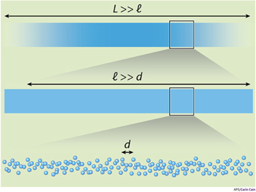
Figure 6. Like any other hydrodynamic approach, GHD applies in the limit where separations of distance and time scales hold. When the characteristic distance L over which densities vary is much larger than the microscopic length scale d, one can view the system as a continuum of locally homogeneous fluid cells of size ℓ (d ≪ ℓ ≪ L) that contain a thermodynamically large number of particles. Similarly, assuming slow variation in time, each fluid cell is locally relaxed to a stationary state. In standard hydrodynamics, this local stationary state is a thermal equilibrium state, while in GHD it is a GGE. Reprinted figure with permission from (Dubail 2016), Copyright 2016 by the American Physical Society.
Download figure:
Standard image High-resolution imageUnder the assumption of separation of scales, the gas is described by its distribution of rapidities ρ(x, θ, t) within each fluid cell [x, x + dx] at time t. This time- and position-dependent rapidity density evolves according to the GHD equations,

These equations were first derived for quantum integrable systems by Bertini et al (2016), Castro-Alvaredo et al (2016) (more precisely, they were derived in the absence of an external potential V(x); the additional term, which corresponds to Newton’s second law, was added later by Doyon and Yoshimura (2017)). These equations are of the same form as equations (4) for the classical integrable gas discussed in the introduction, with two main nuances. The first is that it is the density of rapidities, or asymptotic momenta, that enters the equations, not a ‘bare’ velocity as in the hard rod gas. The second is that  is now the scattering shift (16), which depends on the rapidities, while Δ in the classical gas in the introduction was just a constant equal to minus the diameter of the balls. The effective velocity that solves the second equation (78) can be written as veff[ρ](θ) = iddr(θ)/1dr(θ), as discussed in subsection 1.5.3.
2.1. Hydrodynamic approaches to the 1D Bose gas that preceded GHD
The idea of a hydrodynamic description of the 1D Bose gas does not date back to 2016; it is of course much older. One popular hydrodynamic approach in the atomic gas literature is to start from the Gross–Pitaevskii description of the weakly interacting gas at zero temperature. Writing the wavefunction of the quasicondensate as  , and defining the velocity
  ), one gets the Madelung form of the Gross–Pitaevskii equation (Cazalilla et al
2011, Stringari 1996, 1998),
), one gets the Madelung form of the Gross–Pitaevskii equation (Cazalilla et al
2011, Stringari 1996, 1998),

where 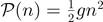 is the pressure of the gas in the quasicondensate regime. Clearly, these two equations look like the first two Euler hydrodynamic equations (3) in the introduction, up to the so-called quantum pressure term
  . This term is beyond the Euler scale though: it involves higher-order derivatives, so in the Euler limit of a slowly varying density n(x), this term vanishes. The reason why there are only two equations in (79), instead of the three Euler equations in the introduction, is that the temperature is zero. Indeed, the third Euler equation in (3) can be recast as a conservation law for the entropy of the fluid, which is automatically satisfied at zero temperature because the entropy identically vanishes.
There have been several attempts at extending this description of the gas beyond the weakly interacting regime, see e.g. (Damski 2006, Kolomeisky et al
2000, Menotti and Stringari 2002). One idea that is often used (Damski 2006, Menotti and Stringari 2002, Öhberg and Santos 2002, Pedri et al
2003, Peotta and Di Ventra 2014, Sarishvili et al
2016) is to replace the pressure  of the quasicondensate regime by the true pressure of the Lieb–Liniger model at zero temperature, calculated from equation (59). This gives a closed system of hydrodynamic equations for the gas that can be solved numerically. This approach can also be used at finite temperature (Bouchoule et al
2016, Doyon et al
2017, Schemmer et al
2019): in that case one numerically solves the three Euler hydrodynamic equations from the introduction with the equilibrium pressure at finite temperature.
of the quasicondensate regime by the true pressure of the Lieb–Liniger model at zero temperature, calculated from equation (59). This gives a closed system of hydrodynamic equations for the gas that can be solved numerically. This approach can also be used at finite temperature (Bouchoule et al
2016, Doyon et al
2017, Schemmer et al
2019): in that case one numerically solves the three Euler hydrodynamic equations from the introduction with the equilibrium pressure at finite temperature.
This ‘conventional’ Euler hydrodynamic approach, which assumes local relaxation of the gas to a thermal equilibrium state, has been successfully applied in states not far from thermal equilibrium, see e.g. (Menotti and Stringari 2002, Öhberg and Santos 2002, Pedri et al 2003). However, it breaks down away from equilibrium. A good illustration of the problems that are typically encountered can be found in (Peotta and Di Ventra 2014), see figure 7. In that reference, the conventional hydrodynamic equations (79) are solved numerically and compared to numerically exact time-dependent density matrix renormalization group (t-DMRG) calculations for small numbers of bosons. The authors find that the hydrodynamic equations can describe the breathing of the atom cloud very well after a quench of the harmonic trapping frequency. However, those hydrodynamic equations are unable to describe a quench from a double-well to a harmonic potential away from the weakly interacting regime.
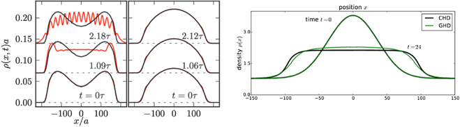
Figure 7. (Left) Evolution of the density profile of the 1D Bose gas after a quench from a double-well to a harmonic potential (left column), and after a quench from harmonic to harmonic, with a different frequency (right column). τ is the oscillation period of the harmonic trap during the evolution. The red curve is obtained by numerically solving the hydrodynamic equation (79) with the pressure  of the Lieb–Liniger model; the black curve is a numerically exact t-DMRG simulation. Clearly, the conventional hydrodynamics (79) works well for the second quench (right column), but not for the first one (left column). Reprinted figure with permission from (Peotta and Di Ventra 2014), Copyright 2014 by the American Physical Society. (Right) Evolution of the density profile from an initial thermal equilibrium state at non-zero temperature in an inverted Gaussian potential
  , which creates an initial density bump. At t > 0 the potential is switched off, V(x) = 0. The density profile evolves according to conventional Euler hydrodynamics (3) at finite temperature (black curve), or according to GHD (green curve). We see that the predictions of both hydrodynamic theories differ at finite temperature (while they would coincide at zero temperature before the appearance of a shock). Reprinted figure with permission from (Doyon et al
2017), Copyright 2017 by the American Physical Society.
, which creates an initial density bump. At t > 0 the potential is switched off, V(x) = 0. The density profile evolves according to conventional Euler hydrodynamics (3) at finite temperature (black curve), or according to GHD (green curve). We see that the predictions of both hydrodynamic theories differ at finite temperature (while they would coincide at zero temperature before the appearance of a shock). Reprinted figure with permission from (Doyon et al
2017), Copyright 2017 by the American Physical Society.
Download figure:
Standard image High-resolution imageThe reason for the failure of this conventional hydrodynamic approach in the latter setup is that it develops a shock after some fraction of the oscillation period. When the atom cloud initially has two well-separated density peaks, some atoms from the left peak move to the right with large velocity, while other atoms from the right peak move to the left with large velocity. Then in the center of the cloud, the fluid is similar to a two-component fluid, with one component moving quickly to the right, the other to the left. Locally, this is a state that is very far from a thermal equilibrium state. The above approach, which enforces local thermal equilibrium, fails to capture that situation. Instead, the Euler-scale hydrodynamic equations (79) develop a shock, which is regulated by higher-order derivative terms, like the quantum pressure term. The solution after the shock depends very strongly on the details of the regularization, so that in general it loses its validity after the first shock. The results of Peotta and Di Ventra (2014) show that the simple insertion of the quantum pressure term into the zero-temperature hydrodynamic equations (79) does not provide the correct regularization for finite repulsion strength. Only in the limit of weak repulsion (g → 0), i.e. when equation (79) is mathematically equivalent to the standard Gross–Pitaevskii equation, does the quantum pressure term provide the right regularization. In that case, the Euler-scale shock is visible in the Gross–Pitaevskii solution through the appearance of strong oscillations of short wavelength in the density profile n(x, t), see e.g. (Simmons et al 2020). These oscillations are beyond the Euler scale, and one can in principle average them over fluid cells to recover the correct Euler-scale description after the shock. Bettelheim (2020) has shown that the Euler-scale dynamics obtained from the Gross–Pitaevskii equation in this way exactly coincides with GHD (at zero temperature and in the limit of weak repulsion).
Away from the Gross–Pitaevskii limit, the analysis carried out in (Doyon et al 2017) shows that the above approach is, in fact, well justified only at zero temperature and before the appearance of the first shock. Moreover, in that case, the conventional hydrodynamics (79) at the Euler scale (i.e. neglecting the quantum pressure term) turns out to be exactly equivalent to GHD. However, in any other situation, it is in principle not applicable, and it leads to quantitatively wrong results. This is illustrated in figure 7.
2.2. Modeling the quantum Newton cradle setup with GHD
Contrary to previous hydrodynamic approaches to the 1D Bose gas, GHD is not based on the assumption of local thermal equilibrium, but only on local relaxation to a stationary state which, in general, is a GGE. This allows the description of situations that are very far from thermal equilibrium. Arguably, the most paradigmatic such out-of-equilibrium situation is the quantum Newton cradle setup of Kinoshita et al (2006). There, the atoms, which are initially at equilibrium in a harmonic potential, are suddenly given a large momentum ±qBragg by a Bragg pulse. Half of the atoms move to the right, the other half move to the left. Because of the harmonic trapping potential, the two packets of atoms oscillate in the trap, colliding twice during each oscillation cycle. In this subsection we review the theoretical work on this paradigmatic setup. The pioneering experiment of Kinoshita et al (2006), which motivated all these theoretical works, is discussed below in section 4.
We stress that, before the advent of GHD, a direct simulation of the quantum Newton cradle setup with experimentally realistic parameters (in particular, number of atoms N ∼ 102–103) was completely out of reach. This is of course because of the exponential growth of the Hilbert space in many-body quantum systems, which makes all direct approaches, such as an exact diagonalization of (a discretized version of) the Lieb–Liniger Hamiltonian (6), numerically intractable for more than a dozen atoms. Thanks to the discovery of GHD in 2016, this situation has now completely changed. Nowadays, it is very easy to model the 1D Bose gas in a quantitatively reliable way.
Bulchandani et al (2017) used GHD to model two packets of atoms colliding against each other on an infinite line. Then, a complete study of the Newton cradle setup, including the trapping potential that gives rise to oscillations of the packets and therefore multiple collisions, was performed by Caux et al (2019), see figure 8. The numerical solution of the GHD equation in that reference was obtained by a classical molecular dynamics simulation of the so-called flea gas model (Doyon et al 2018), which is an extension of the classical hard rod gas that incorporates the scattering shift discussed in subsection 1.1. There are other ways of numerically solving the GHD equations, which have been discussed, to some extent, in (Bastianello et al 2019, Bastianello et al 2020a, Bulchandani et al 2017, 2018, Doyon et al 2017, Møller and Schmiedmayer 2020, Møller et al 2021) (see also the appendix of the review by Bastianello et al (2021) in this volume). Among these works, we draw the reader’s attention in particular to the GHD code ‘iFluid’ of Møller and Schmiedmayer (2020), which is publicly available.
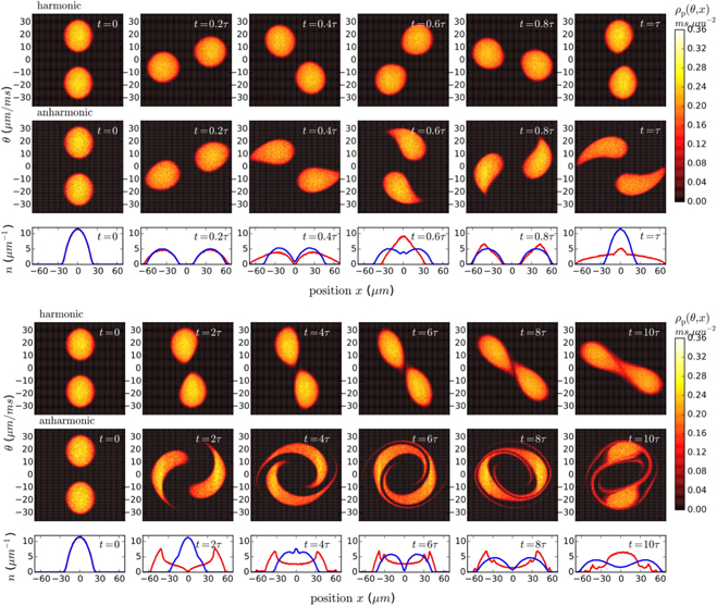
Figure 8. GHD simulation of the 1D Bose gas in the Newton cradle setup. (Top) The evolution of the phase-space rapidity density ρ(x, θ, t) during the first oscillation cycle is shown for a harmonic trap with period τ (first row), and a quasi-harmonic trap with a small anharmonicity (second row). The corresponding density profiles n(x, t) = ∫ρ(x, θ, t)dθ are shown in blue and red respectively (third row). (Bottom) Same as the top, but on longer time scales. Reproduced from (Caux et al 2019). CC BY 4.0.
Download figure:
Standard image High-resolution imageIn figure 8, one can observe the evolution of the rapidity distribution predicted by GHD in a harmonic potential  (with oscillation period τ = 2π/ω), and also in a potential with a small anharmonicity
  . The initial state is constructed so as to mimic the effect of the Bragg pulse sequence that imparts the initial momentum to the atoms. Before the sequence, the gas is described in a hydrostatic (or local density) approximation by its local distribution of rapidities ρ(x, θ, t < 0) = ρthermal(x, θ), obtained by solving the Yang–Yang equation (57) for a thermal equilibrium distribution. Then momentum ±qBragg is imparted in a random fashion to all quasiparticles in the system. This results in a distribution of rapidities at t = 0

This simple ansatz for the initial state can be justified using the results of van den Berg et al (2016), which showed that the momentum distribution function of the bosons is affected in this way by a Bragg pulse, and to a good approximation the same holds for the rapidities. The rapidity distribution is evaluated at later times by solving the GHD equation (78). One observes that the two blobs, initially well separated in momentum space for sufficiently large qBragg, evolve by performing a deformed rotation-like movement around the origin of phase space. In the harmonic case, over the first two or three oscillation cycles, their evolution is not drastically affected by the collisions. However, at later times the two blobs ultimately merge due to inter-cloud interactions. With a small anharmonicity, the two blobs get deformed much more quickly and the distribution ρ(x, θ, t) gets more and more stirred up after a few periods. This dephasing effect would also be present for the single particle in an anharmonic trap, see e.g. (Bastianello et al 2017). Many-body dephasing is also present: without interactions, the original blobs would disintegrate into long spiraling filaments; instead, here the filaments merge and high-energy (longer-period) tails scatter to lower energies, leading to the reformation of new blobs.
Importantly, the ability to perform GHD modeling of the Newton cradle setup has opened the possibility of studying theoretically one fundamental question raised by the experiment of Kinoshita et al (2006). If one waits long enough, does the gas in the trap ultimately reach thermal equilibrium?
This question is non-trivial because, although the Lieb–Liniger gas is integrable, its integrability is broken by the trapping potential V(x). Yet, at the Euler scale, the potential V(x) varies very slowly compared to microscopic scales, so the breaking of integrability by the external potential is weak. It is not obvious how much of the original conservation laws should be reflected in the stationary state.
Cao et al (2018) studied this question for the classical hard rod gas in a trapping potential, and found that the answer is negative: the gas exhibits ‘incomplete thermalization’. It reaches a stationary state of the GHD equation (78), namely a rapidity distribution ρstat.(x, θ) which satisfies

but this distribution does not need to be a thermal equilibrium distribution in the trap. The possibility of GHD-stationary distributions of the form (81) that are not thermal has also been discussed in (Doyon and Yoshimura 2017). Caux et al (2019) arrived at the same conclusion for the 1D Bose gas in the Newton cradle setup, within the framework of the aforementioned flea gas model. In (Caux et al 2019), the existence of non-thermal stationary states was argued to be a consequence of the conservation of certain quantities S[f] under evolution generated by the Euler-scale GHD equation (78), even in the presence of an external potential V(x). The conservation of these quantities is incompatible with convergence toward thermal equilibrium. These quantities can be constructed out of the Fermi occupation ratio ν(x, θ, t), and read

for arbitrary functions f. We stress that these quantities are different from the standard conserved charges of the form (28). Instead, the quantities S[f] look more like generalizations of the Yang–Yang entropy: the Yang–Yang entropy, integrated over space, corresponds to the specific choice f(ν) = −ν log ν − (1 − ν) log(1 − ν), see equation (49). The fact that

can be checked directly using the GHD equation (78), see (Caux et al 2019). We stress that the Yang–Yang entropy, and more generally the quantities S[f], are conserved only at the Euler scale. When higher-order terms are included into the hydrodynamic equations (78), as discussed in subsection 2.4.3 below, the entropy increases with time, and the other quantities S[f] are no longer constant. In particular, it has been argued recently by Bastianello et al (2020a) that the inclusion of a Navier–Stokes-like higher-order term in (78) does lead to ‘complete thermalization’, see subsection 2.4.3 below.
2.3. Other setups
Let us briefly review some other physically relevant setups that have been investigated with the new toolbox provided by GHD.
De Nardis and Panfil (2018) considered the case of two atom clouds that are prepared at different temperatures T1 ≠ T2, put in the same trapping potential. At the junction between the two clouds, the local state displays an edge singularity in its response function and quasilong-range order.
Dubessy et al (2021) studied the Lieb–Liniger gas in an infinite flat box potential (figure 9). Initially the gas is in its ground state. At time t = 0, it is instantaneously boosted by a momentum k0, a protocol that can be realized experimentally by phase imprinting. Then the particles in the gas start reflecting against the two infinite walls at x = 0 and x = L. This is modeled in GHD by the following boundary condition:

The same boundary condition holds at x = L. Dubessy et al (2021) used a trick to implement easily these boundary conditions: the system can be glued together with its mirror image, to give a periodic system of length 2L. The rapidity distribution in that periodic system of size 2L is related to that in the infinite box potential by

With this trick, Dubessy et al (2021) studied the formation of shock waves that oscillate in the box for several periods, with a period fixed by the sound velocity in the gas, see figure 9.
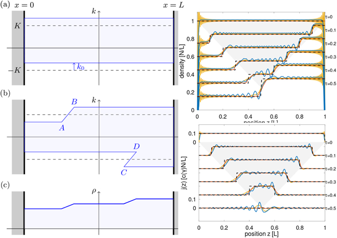
Figure 9. (Left) GHD simulation of a gas in a box trap. (a) The initial state is the ground state, on which a boost of +k0 is applied at t = 0. The blue region is the region of phase space where the Fermi occupation ratio ν(x, θ, t) = ρ(x, θ, t)/ρs(x, θ, t) is one. Outside this region, it is zero. (b) After some time the contour of the blue region gets deformed. (c) The corresponding real-space density profile n(x, t) = ∫ρ(x, θ, t)dθ. (Right) Evolution of the particle density (top) and current (bottom). Here τ = t/(vL) where v is the sound velocity. The blue curve is obtained with the Gross–Pitaevskii equation (valid for small γ), the yellow curve is obtained from a free fermion calculation in the γ → ∞ limit, and the red curve is the GHD simulation at γ = 1. The dashed black line corresponds to an effective model. Reproduced from (Dubessy et al 2021). CC BY 4.0.
Download figure:
Standard image High-resolution imageDoyon et al (2017) pointed out that a drastic simplification of the GHD equations occurs when the gas is initially in its ground state. In an external potential V(x), the ground state is modeled by hydrostatics, or equivalently by the local density approximation (LDA), which gives the distribution of rapidities ρ(x, θ, t = 0). In the ground state, the Yang–Yang entropy of the gas vanishes. Then, since entropy is always conserved by Euler-scale hydrodynamic equations, it must vanish at all times. This puts very strong restrictions on the class of local stationary states that are explored by the system under GHD evolution: these local states must be either the ground state itself (up to a Galilean boost), or a ‘split Fermi sea’ (Eliëns 2017, Eliëns and Caux 2016, Fokkema et al 2014). Within the framework of GHD, this is easily understood by using the so-called convective form of the GHD equation (78), which gives the evolution of the Fermi occupation ratio ν(x, θ, t) = ρ(x, θ, t)/ρs(x, θ, t),

(It is easy to see that this form of the GHD equation is equivalent to (78). Plugging the constitutive relation (41) into (78), one finds that the first equation (78) satisfied by ρ(x, θ, t) is also satisfied by ρs(x, θ, t). This directly leads to (86) for the ratio ρ/ρs.)
In the ground state, the Fermi occupation ratio is either zero or one: ν(x, θ) = 1 if θ ∈ [−θF(x), θF(x)], and ν(x, θ) = 0 otherwise. Here θF(x) is a position-dependent Fermi momentum, which depends on the atom density n(x), see subsection 1.5. This specific form of ν(x, θ, t) is preserved under (86): at any time, ν(x, θ, t) is either zero or one. Consequently, the state of the system at time t is parameterized by a contour Γt in phase space (figure 9, left, and figure 13, top row), which separates the region where ν = 1 from the one where ν = 0, namely

Writing the contour as Γt = {(xt (s), θt (s)); s ∈ [0, 2π)}, and plugging this into equation (86) one finds that its evolution equation reads

This ‘zero-entropy GHD’ (Doyon et al 2017) is very useful for numerical purposes, because it provides a very efficient way of solving the GHD equations: it is easier to compute the evolution of the contour Γt , rather than to simulate the evolution of the full distribution ρ(x, θ, t), even though both formulations are equivalent in the end. In figure 13 (top row), one can see the evolution of the contour Γt when the gas is suddenly released from its ground state in a double-well potential to a harmonic potential. After a fraction of the period of the harmonic trap frequency, one observes the appearance of local split Fermi seas. Hence, such a setup could not be described by the conventional hydrodynamic approaches of subsection 2.1, because the appearance of such multiple Fermi seas would translate into shock formations in those approaches. GHD, on the other hand, does not have shocks (Bulchandani 2017, Doyon et al 2017, El and Kamchatnov 2005) and remains valid after the appearance of multiple Fermi seas.
2.4. Extensions of Euler-scale GHD
So far we have reviewed results obtained on the 1D Bose gas with the Euler-scale GHD equation (78). Since 2016, the original framework has been extended in several directions that could be relevant to the description of existing or future experiments. We now turn to these developments.
2.4.1. Adiabatically varying interactions
The original formulation of GHD of Bertini et al (2016), Castro-Alvaredo et al (2016) was for a time-independent translation invariant Hamiltonian acting on a spatially inhomogeneous state. In particular, no external potential term −(∂x V)(∂θ ρ) was included originally. Doyon and Yoshimura (2017) considered the addition of generalized potentials to the Hamiltonian H → H + ∫Vf (x)q[f](x)dx, where q[f](x) is the charge density of the charge operator (28). This includes, in particular, the case of a standard external potential H → H + ∫V(x)Ψ†(x)Ψ(x)dx, corresponding to the simplest choice q[f] = 1, which results in the form (78) of the GHD equation with the acceleration term −∂x V∂θ ρ. This is the form of the GHD equation that is most relevant for the description of existing experiments. However, we stress that the results of Doyon and Yoshimura (2017) are in principle more general.
A further extension of the original GHD equation was obtained by Bastianello et al (2019), who considered the case of a non-uniform repulsion strength g(x, t) through the gas, see figure 10. Under the assumption of slow variation of g(x, t) (or of 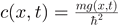 ) in position and time, they found the following additional term:

where we have dropped the dependence on x, θ and t for better readability, and where the functions F and Λ are

For a derivation of this result, see the original paper (Bastianello et al 2019).
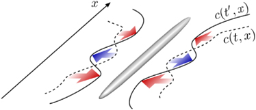
Figure 10. The GHD equations (78) can be extended to include an repulsion strength c(x, t) that varies slowly in time or in space, which would correspond to slowly varying the transverse trapping frequency in an experimental setup. Reprinted figure with permission from (Bastianello et al 2019), Copyright 2019 by the American Physical Society.
Download figure:
Standard image High-resolution image2.4.2. Boltzmann kinetic equation for a Bose gas at the 1D–3D crossover
Taking inspiration from the developments of GHD, Møller et al (2021) studied a three-dimensional (3D) Bose gas at the crossover to the 1D regime, and introduced a phenomenological description of the gas dynamics at that crossover. The idea is the following. The atoms lie in the 3D potential V(x) + V⊥(r⊥), where  is the distance from the axis at y = z = 0. The transverse potential is harmonic,
  , so that the wavefunction of each atom ψ(x, r⊥) can be expanded on the eigenstates ψn
(r⊥) of the transverse harmonic oscillator, see equation (103) below. Strictly in the 1D regime (i.e. when ℏω⊥ is much larger than all other energy scales), the transverse ground state (n = 0) is the only state that is occupied. But if the transverse confinement is not strong enough, transversely excited states will also be occupied. Møller et al (2021) consider the first three transverse states (n = 0, 1, 2) (their degeneracy is neglected), and regard the resulting system as a three-component 1D Bose gas, with a Hamiltonian of the form
, so that the wavefunction of each atom ψ(x, r⊥) can be expanded on the eigenstates ψn
(r⊥) of the transverse harmonic oscillator, see equation (103) below. Strictly in the 1D regime (i.e. when ℏω⊥ is much larger than all other energy scales), the transverse ground state (n = 0) is the only state that is occupied. But if the transverse confinement is not strong enough, transversely excited states will also be occupied. Møller et al (2021) consider the first three transverse states (n = 0, 1, 2) (their degeneracy is neglected), and regard the resulting system as a three-component 1D Bose gas, with a Hamiltonian of the form

Here the excitation terms are of the form  and correspond, for instance, to a two-body collision where two atoms in the transverse ground state get excited to the first excited state. The coupling constants ga
and gab
(a, b = 0, 1, 2) are effective 1D coupling constants resulting from the 3D interaction. For a 3D scattering length much smaller than
and correspond, for instance, to a two-body collision where two atoms in the transverse ground state get excited to the first excited state. The coupling constants ga
and gab
(a, b = 0, 1, 2) are effective 1D coupling constants resulting from the 3D interaction. For a 3D scattering length much smaller than  , they can be calculated from the shape of the transverse orbitals, see the discussion in subsection 3.1.2. Møller et al (2021) simply assume that they are equal: ga
= gab
= g. Under that assumption, the multi-component Bose gas with V(x) = 0 is integrable (Caux et al
2009, Gaudin 2014, Klauser and Caux 2011, Klümper and Pâţu 2011, Pâţu and Klümper 2015, Robinson et al
2016, Robinson and Konik 2017, Yang 1967), however, the description of its thermodynamic limit is considerably more complicated than that given by the Lieb–Liniger model reviewed in section 1. In particular, while the macrostates of the Lieb–Liniger model in the thermodynamic limit are characterized by their distribution of rapidities ρ(θ), those of the multi-component Bose gas are characterized not only by ρ(θ), but also by infinitely many rapidity distributions for pseudo-spin bound states. Møller et al (2021) assume that the population of such pseudo-spin bound states is small and can be neglected, and keep only the distribution of rapidities ρ(θ), whose evolution under the Hamiltonian (90) then coincides with that of the Lieb–Liniger gas, and is therefore nothing but the GHD equation (78).
, they can be calculated from the shape of the transverse orbitals, see the discussion in subsection 3.1.2. Møller et al (2021) simply assume that they are equal: ga
= gab
= g. Under that assumption, the multi-component Bose gas with V(x) = 0 is integrable (Caux et al
2009, Gaudin 2014, Klauser and Caux 2011, Klümper and Pâţu 2011, Pâţu and Klümper 2015, Robinson et al
2016, Robinson and Konik 2017, Yang 1967), however, the description of its thermodynamic limit is considerably more complicated than that given by the Lieb–Liniger model reviewed in section 1. In particular, while the macrostates of the Lieb–Liniger model in the thermodynamic limit are characterized by their distribution of rapidities ρ(θ), those of the multi-component Bose gas are characterized not only by ρ(θ), but also by infinitely many rapidity distributions for pseudo-spin bound states. Møller et al (2021) assume that the population of such pseudo-spin bound states is small and can be neglected, and keep only the distribution of rapidities ρ(θ), whose evolution under the Hamiltonian (90) then coincides with that of the Lieb–Liniger gas, and is therefore nothing but the GHD equation (78).
Finally, the effects of the excitation terms in the Hamiltonian (90) are introduced in the form of a Boltzmann collision integral:

The collision integral  is constructed phenomenologically, by considering a simple model for two-body collisions. This phenomenological approach does not incorporate interactions with the other particles, contrary to what usually happens in exact Bethe ansatz calculations (where the interaction effects appear through the dressing of the various quantities that enter all the formulas). Within the framework of that very simple model, the probability of two colliding atoms with momenta p1 = ℏk1, p2 = ℏk2 initially in the same transverse state getting excited to a different transverse state is estimated as P↕(k, q) ≃ 4c2
kq/[k2
q2 + c2(k + q)2] where k = |k1 − k2| and
is constructed phenomenologically, by considering a simple model for two-body collisions. This phenomenological approach does not incorporate interactions with the other particles, contrary to what usually happens in exact Bethe ansatz calculations (where the interaction effects appear through the dressing of the various quantities that enter all the formulas). Within the framework of that very simple model, the probability of two colliding atoms with momenta p1 = ℏk1, p2 = ℏk2 initially in the same transverse state getting excited to a different transverse state is estimated as P↕(k, q) ≃ 4c2
kq/[k2
q2 + c2(k + q)2] where k = |k1 − k2| and  . Then the authors assume that the atom momenta may be replaced by the rapidities, and arrive at an expression of the form
 ![$\mathcal{I}\propto {\sum }_{n=1,2}[{\mathcal{I}}_{\text{h}}^{-}{\nu }_{n}^{{\beta }_{n}}-{\mathcal{I}}_{\text{p}}^{-}-{\mathcal{I}}_{\text{p}}^{+}{\nu }_{n}^{{\beta }_{n}}+{\mathcal{I}}_{\text{h}}^{+}]$](https://content.cld.iop.org/journals/1742-5468/2022/1/014003/revision6/jstatac3659ieqn119.gif) , where νn
is the probability that an atom is in the nth transversely excited state (assumed to be ≪1 for n = 1, 2), βn
is the number of atoms changing state in a collision (β2 = 1 and β1 = 2 in the model of Møller et al (2021)), and
, where νn
is the probability that an atom is in the nth transversely excited state (assumed to be ≪1 for n = 1, 2), βn
is the number of atoms changing state in a collision (β2 = 1 and β1 = 2 in the model of Møller et al (2021)), and

with similar expressions for  ,
,  and
and  , where the indices ‘p’ and ‘h’ refer to ‘particle’ and ‘hole’, see (Møller et al
2021). Here
, where the indices ‘p’ and ‘h’ refer to ‘particle’ and ‘hole’, see (Møller et al
2021). Here  are the momenta of the two atoms after getting excited to the transverse state in that model of two-body collisions.
The various approximations involved in the construction of the effective Boltzmann equations (91) and (92) are particularly meaningful in the ideal Bose gas regime. There, this phenomenological approach is expected to work well. Notice that in the ideal Bose gas regime, the GHD dynamics reduces to that of free Bosons, with the effective velocity appearing in equation (91) reducing to the bare velocity veff(θ) = θ/m. In that regime the aforementioned assumption that all intra- and inter-component coupling strengths are equal is actually no longer necessary for the gas to be integrable. Beyond the ideal Bose gas regime, the accuracy of the description of the 1D–3D crossover by equations (91) and (92) remains to be investigated.
Motivated by the recent experiment in the Newton cradle setup of Li et al (2020), which observed thermalization attributed to excitations of the transverse modes, Møller et al (2021) simulated the Newton cradle with equations (91) and (92) in the ideal Bose gas regime, and found that excitations to the transverse modes do indeed induce thermalization, see figure 11.
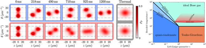
Figure 11. (Left) Evolution of the rapidity distribution ρ(θ) under GHD in the quantum Newton cradle setup (top), compared to the equation (91) that includes a phenomenological Boltzmann collision integral modeling excitations to transverse modes when the gas is at the 1D–3D crossover. (Right) The cloud is initially in the ideal Bose gas regime, and it stays in that regime under time evolution with equation (91). Reprinted figure with permission from (Moller et al 2021), Copyright 2021 by the American Physical Society.
Download figure:
Standard image High-resolution image2.4.3. Beyond the Euler scale: Navier–Stokes diffusive corrections
As mentioned in the introduction, Euler-scale hydrodynamic equations are but the zeroth order in a gradient expansion. More precisely, under the assumption of local relaxation, the expectation values of the currents  are functions of the charges
  and of their derivatives. Schematically,
  , which is then expanded as
  . The zeroth order gives the Euler-scale hydrodynamic equations, while the next order gives the hydrodynamic equation at the diffusive scale. These hydrodynamic equations include a diffusive, entropy-producing (or Navier–Stokes) term.
The ‘Navier–Stokes’ GHD equation, with the diffusive term, was obtained in (De Nardis et al 2018). The result reads

where  is a kernel (i.e.
  ) describing a Markov process of random momentum exchanges via two-body collisions (De Nardis et al
2019, Gopalakrishnan et al
2018). It is defined by the relation
) describing a Markov process of random momentum exchanges via two-body collisions (De Nardis et al
2019, Gopalakrishnan et al
2018). It is defined by the relation

with

For a detailed derivation of these equations, see (De Nardis et al 2019).
As mentioned above, interestingly, taking into account the diffusive correction changes the conclusion about thermalization in the quantum Newton cradle setup, see (Bastianello et al 2020a) and figure 12. With the inclusion of the Navier–Stokes term, the quantities (82) are no longer conserved, and it is found that the gas ultimately reaches thermal equilibrium, contrary to what had been observed previously in (Cao et al 2018, Caux et al 2019).
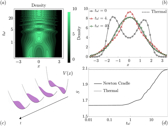
Figure 12. When the Navier–Stokes term (93) is included in the GHD equation, it is found that the 1D Bose gas in the quantum Newton cradle does reach thermal equilibrium. (a) Evolution of the density profile n(x, t) under GHD–Navier–Stokes evolution. In (b), one sees that the density goes to the thermal equilibrium density at long times. (c) Illustration of the quench protocol (quench from a double-well to a harmonic potential). (d) The entropy increases and ultimately reaches its thermal equilibrium value. Reprinted figure with permission from (Bastianello et al 2020), Copyright 2020 by the American Physical Society.
Download figure:
Standard image High-resolution imageFor more studies of diffusion in the Lieb–Liniger gas, see e.g. (Medenjak et al 2020, Panfil and Pawełczyk 2019). Diffusion has also been studied very extensively in spin chains; for this topic we refer the reader to the review articles by Bulchandani et al (2021) and by De Nardis et al (2021) in this volume.
2.4.4. Quantum fluctuating hydrodynamics
As emphasized above, Euler-scale hydrodynamic equations are based on separation of scales (figure 6), which allows for a description of the gas as a continuum of independent fluid cells, each of which has relaxed to a stationary state.
In that hydrodynamic picture, a small perturbation of the system at spacetime position (x, t) generates sound waves that propagate through the gas, so that the perturbation may be observable at a different position (x′, t′) (Kadanoff and Martin 1963). Such dynamical correlations have been studied in the framework of GHD in (Doyon 2018, Møller et al 2020); see also the review by De Nardis et al (2021) in this volume.
However, at equal time, the fluid cells at different positions x and x′ are independent. Thus, all equal-time connected correlations vanish at the Euler scale: for any local observables  ,
,

This is somewhat puzzling because, in a quantum system, equal-time correlations are typically non-zero: for instance, in the ground state of the Lieb–Liniger gas they are non-zero, see e.g. the reviews (Cazalilla 2004, Cazalilla et al 2011). However, this is not in contradiction with (95): the reason is simply that such non-zero equal-time correlations are an effect occurring beyond the Euler scale.
A good illustration of this phenomenon is provided by the standard fluid described by the Euler equations (3). At zero temperature, the third Euler equation (3) is automatically satisfied as a consequence of the first two (see the discussion in subsection 2.1), so we are left with

For simplicity, we now consider the ground state of the spatially homogeneous system (V(x) = 0), with n(x, t) = n and u(x, t) = 0. Linearizing the system (96) around that solution leads to the equation of propagation of sound waves (δn(x, t), δu(x, t))

or equivalently

Here v is the sound velocity in the gas, and K is a dimensionless parameter (called the Luttinger parameter, see below) normalized such that K → 1 in the hard-core limit. We see from equation (98) that there are right- and left-moving sound waves, corresponding to specific linear combinations of δn and δu parameterized by K, traveling at velocity ±v.
The sound waves can be used as the basic ingredient in a quantized theory of the fluid described by the Euler equations (96). The basic idea is to view δn(x) and δu(y) as operators in a quantum theory, and to impose the canonical commutation relations of a one-component fluid (Landau 1941),

and ![$\left[\delta n(x),\delta n(y)\right]=\left[\delta u(x),\delta u(y)\right]=0$](https://content.cld.iop.org/journals/1742-5468/2022/1/014003/revision6/jstatac3659ieqn131.gif) . Then, one should find a Hamiltonian H such that the Heisenberg equations
. Then, one should find a Hamiltonian H such that the Heisenberg equations ![${\partial }_{t}\delta n=\frac{\text{i}}{\hslash }[H,\delta n]$](https://content.cld.iop.org/journals/1742-5468/2022/1/014003/revision6/jstatac3659ieqn132.gif) and
and ![${\partial }_{t}\delta u=\frac{\text{i}}{\hslash }[H,\delta u]$](https://content.cld.iop.org/journals/1742-5468/2022/1/014003/revision6/jstatac3659ieqn133.gif) coincide with the equations of motion (97). The simplest choice is:
coincide with the equations of motion (97). The simplest choice is:

which is nothing but the Hamiltonian of a Luttinger liquid, see e.g. (Cazalilla 2004, Giamarchi 2003, Tsvelik 2007) for introductions. Thus, we see that quantizing the sound waves of a standard Euler fluid at zero temperature (96) directly leads to a Luttinger liquid. With that observation, one can get the leading behavior of equal-time correlations beyond the Euler scale. For instance, the equal-time density–density correlation in the ground state of the Hamiltonian (100) is (Cazalilla 2004, Giamarchi 2003, Tsvelik 2007):

Such correlation functions can then be propagated in time using the sound wave equation (98). For instance, propagating equation (101) in time leads to a combination of two terms, one coming form the right-moving sound wave, the other from the left-moving one:

Other time-dependent correlations can be obtained in a similar way within the framework of Luttinger liquid theory, see e.g. (Cazalilla 2004, Giamarchi 2003, Tsvelik 2007). These dynamical correlation functions obtained from the propagation of linear sound waves are valid on time scales that are not too long, before non-linear effects kick in. For a review on such non-linear effects, see (Imambekov et al 2012).
It is natural to ask whether such a program can be implemented, replacing the standard Euler equations at zero temperature (96) by those of GHD at zero temperature (88). This was achieved, to some extent, by Ruggiero et al (2020). In this work, the equations for linear sound waves around zero-entropy GHD are derived, and quantized by imposing canonical commutation relations. This procedure results in a time-dependent, spatially inhomogeneous, multi-component Luttinger liquid.
In the ground state of the gas, the Hamiltonian obtained by Ruggiero et al (2020) is that of an inhomogeneous Luttinger liquid, see e.g. (Bastianello et al 2020c, Brun and Dubail 2018, Cazalilla 2004, Dubail et al 2017). At later times it follows the evolution of the system under the zero-entropy GHD equation (88), encoding the propagation of the quantum fluctuations from time t = 0 to times t > 0, see figure 13. For more details we refer the reader to (Collura et al 2020, Ruggiero et al 2019, 2020), and to the review by Alba et al (2021) in this volume.
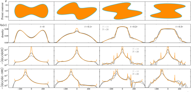
Figure 13. Quench from a double-well to a harmonic potential (with period τ) in a 1D Bose gas at zero temperature and γ ≃ 1. Top row: evolution of the contour Γt
according to the zero-entropy GHD equation (88). Second row: the corresponding density profiles n(x, t) (orange), compared to t-DMRG results for N = 10 and N = 20 particles. Third and fourth rows: the equal-time density–density correlation function  obtained by quantizing the sound waves around zero-entropy GHD. Reprinted figure with permission from (Ruggiero et al
2020), Copyright 2020 by the American Physical Society.
obtained by quantizing the sound waves around zero-entropy GHD. Reprinted figure with permission from (Ruggiero et al
2020), Copyright 2020 by the American Physical Society.
Download figure:
Standard image High-resolution imageWe also mention that there is, in principle, another approach to quantum fluctuations in GHD (Fagotti 2017, 2020), which consists of viewing the GHD equation (78) as the zeroth order in the evolution equation for the Wigner quasiprobability distribution (Bettelheim et al 2006, Bettelheim and Glazman 2012, Bettelheim and Wiegmann 2011, Dean et al 2018, 2019, Doyon et al 2017, Fagotti 2020, Moyal 1949, Protopopov et al 2013, Ruggiero et al 2019). The evolution equation of the Wigner function may be expanded in powers of ℏ (Moyal 1949), with higher-order terms that give the corrections to the Euler-scale GHD equation. In this approach, it is not only the quantum fluctuations at time zero that are propagated in time as above. Corrections also appear dynamically because of the modified evolution equation. So far, this approach has been limited to the hard-core limit g → +∞, or more generally to spin chains that map to non-interacting fermions. To our knowledge, the extension of this approach to the interacting case is an open problem. We refer the reader to the aforementioned review by Alba et al (2021) in this volume for a thorough discussion of this topic.
3. The 1D Bose gas in cold atom experiments
Cold atom setups are well adapted to the study of model systems in many-body physics. First, because of the small energy scales and large inter-particle distances, the interactions in cold atom systems can be modeled by simple terms. In particular, in many cases, the two-body interactions are well represented by a contact interaction characterized by its scattering length. Second, cold atom gases are extremely well isolated from their environment. Third, the different parameters controlling the physics, such as the interaction strength g, or the external potential V(x), are controllable with great flexibility. For these reasons, cold atom setups are ideal for simulating many-body Hamiltonians, and in particular they can be used to investigate the physics of 1D Bose gases with contact interactions. In this section we briefly review the main ideas and results that have led to these experimental achievements.
3.1. The 1D regime
3.1.1. One-dimensional geometries
Confining potentials for cold atoms can be realized by different means (see for instance the book by Pethick and Smith (2008)). One can use laser fields: the interaction between the induced atomic dipole and the laser field results in a force acting on the center-of-mass motion of the atom, which is conservative if the laser frequency is sufficiently far from any atomic resonance and which is proportional to the laser intensity gradient. One can also rely on a non-vanishing magnetic moment of the atoms to realize potentials using spatially varying magnetic fields. For large enough magnetic fields, adiabatic following of the orientation of the magnetic dipole of the atoms ensures the realization of conservative potentials.
One-dimensional gases are realized in cold atom setups when the atoms are confined in guides with a transverse confinement large enough that the energy gap between the transverse ground state and the first excited state is much larger than the typical energy per atom. Then the transverse degrees of freedom get frozen and the resulting dynamics are effectively 1D. The strong transverse confinement required to reach the 1D regime can be realized using laser fields with large intensity gradients resulting from interference: a two-dimensional (2D) optical lattice formed by lasers far-detuned from the atomic transitions realizes a 2D array of 1D tubes for the atoms where the 1D regime can be accessed (Fabbri et al 2011, Haller et al 2009, Kinoshita et al 2005), see figure 14. Such setups present several advantages. First, they offer the possibility of realizing very strong transverse confinements, since the light intensity is modulated at distances as small as the laser wavelength. Second, cold atoms are loaded into such a lattice adiabatically from a 3D Bose–Einstein condensate (BEC), which permits one to obtain very cold 1D gases. Finally, in this setup the magnetic field is a free parameter that can be tuned to approach Feshbach resonances and thus adjust the interaction strength between atoms (Haller et al 2009). On the other hand, optical lattice setups also have some limitations. The first is that all measurements are ensemble measurements: the value of the measured observable is averaged over several 1D tubes, with parameters such as the number of atoms or the interaction strength varying from tube to tube, which complicates the data analysis. This averaging also prevents the investigation of fluctuations and correlations. Second, the 2D optical lattice has a finite length in the longitudinal direction—the direction along the tubes—since it is produced using lasers with relatively small waists. This imposes restrictions on the spatial extension of the 1D gases: the clouds cannot be too long. However, this limitation does not prevent cloud expansions that are long enough to allow access to the rapidity distribution, see section 3.3.
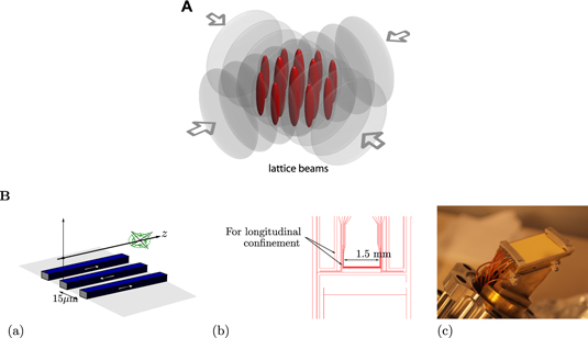
Figure 14. Creating 1D gases in cold atom experiments. (A) A 2D optical lattice produces an array of 1D tubes. From (Haller et al 2009). Reprinted with permission from AAAS. (B) Guiding atoms along a three-wire guide on an atom chip (pictures from the atom chip setup in Palaiseau, France). (a) Three parallel wires, running current in alternate directions, guide the atoms along a line above the central wire. (b) Chip layout (wire edges shown). In addition to the three-wire guide, other wires are used for the longitudinal confinement and for preparation stages. (c) The atom chip, covered with a gold mirror.
Download figure:
Standard image High-resolution imageAnother type of experiment uses magnetic trapping of atoms to reach the 1D regime. Strong magnetic gradients are obtained in the vicinity of microwires running an electrical current in the so-called atom chip setup first developed in Munich (Reichel et al 1999) and in Vienna (Folman et al 2000) (see (Reichel and Vuletic 2011) for a review). Close enough to the microstructures, the 1D regime can be reached (Armijo et al 2011, Jacqmin et al 2011, van Amerongen et al 2008). The idea of magnetic guiding is simple. Consider a current-carrying wire immersed in a homogeneous magnetic field which is perpendicular to it. The total magnetic field vanishes on a line parallel to the wire, and atoms, when polarized in a low-field seeker magnetic state, will be guided along this line. The transverse homogeneous magnetic field can be replaced by the magnetic field produced by two wires placed on each side of the central wire, so that one has the configuration depicted in figure 14. Strong transverse confinement is obtained close to the wires and, in some experiments, atoms are guided at a distance of as small as 15 μm from the wires (Jacqmin et al 2011). The advantage of atom chip setups is that a single 1D gas is realized and studied. This allows direct comparison with theoretical predictions. This also permits the study of fluctuations, and of their correlations. The guiding of atoms can be realized on very long distances, as the transverse confinement is invariant along the whole microwire. However, atom chips also have some drawbacks. In particular, the 1D gases are prepared and cooled down directly in the 1D geometry, and it turns out that temperatures obtained in these setups are higher than those obtained using 2D optical lattices. The physical phenomena limiting the temperatures that can be reached are not completely elucidated, although the role of atom losses has recently been singled out (Bouchoule and Schemmer 2020, Rauer et al 2016, Schemmer and Bouchoule 2018).
3.1.2. Effective 1D interaction parameter
In experiments, although the transverse confinement is large enough to freeze the transverse degrees of freedom, it is typically small enough that the width of the transverse ground state wavefunction is much larger than the range of the 3D interaction potential. In that case, one can model the 3D interaction by a contact potential characterized by the scattering length a3D. The relation between the 3D scattering properties and the 1D scattering properties was worked out by Olshanii (1998), and we briefly review the main steps of his argument. A harmonic transverse confinement of frequency ω⊥ is assumed, and the scattering state of two atoms is explicitly constructed. Because of the harmonic nature of the transverse confinement, the center-of-mass motion decouples from that of the relative coordinate. The wavefunction of the relative coordinate obeys the Schrödinger equation for a particle of mass m/2 in a harmonic transverse confinement of frequency ω⊥ and with the 3D contact potential at the origin. It can be expanded as a sum of transverse eigenstates, with x-dependent amplitudes. One considers a state whose energy is small enough that, apart from the transverse ground state, the amplitudes are exponentially decreasing functions of x. Then the 3D wavefunction reads,

where the sum runs over the transversely excited states of vanishing angular momentum whose wavefunctions are ψn (r⊥), where r⊥ is the transverse distance to the origin. The parameters {an } and δ are determined in the following way. First, one imposes that ∂ψ/∂x is regular everywhere in the plane x = 0 except at the 3D origin. Then, one imposes that the wavefunction fulfills the 3D boundary condition: for a zero-range 3D interacting potential of scattering length a3D, the wavefunction diverges as 1/r − 1/a3D at short distance. This fixes the value of tan(δ), which is found to scale as 1/k at small k (Olshanii 1998). For a pure 1D problem, with a contact potential g1D δ(x), one would have tan(δ) = −mg1D/(2ℏ2 k). Comparing with the small k limit of the 3D problem, one finds that the effective 1D coupling constant is (Olshanii 1998)

where  is the width of the transverse ground state and
  .
.
In most experimental realizations, a3D ≪ a⊥, so that Olshanii’s relation (104) reduces to g1D = 2ℏω⊥
a3D. This expression can be recovered by simple reasoning, valid for a weakly interacting gas in the quasicondensate regime. Since we assume a3D ≪ a⊥, interactions have a 3D nature and their effect is obtained simply by averaging over the transverse density profile. More precisely, the interaction energy per unit length in the longitudinal direction is  , where g3D = 4πℏ2
a3D/m is the 3D interaction strength. On the other hand, considering the 1D problem one obtains
, where g3D = 4πℏ2
a3D/m is the 3D interaction strength. On the other hand, considering the 1D problem one obtains  . Equating both expressions, and using the Gaussian shape of ψ0, one recovers g1D = 2ℏω⊥
a3D.
. Equating both expressions, and using the Gaussian shape of ψ0, one recovers g1D = 2ℏω⊥
a3D.
Equation (104) shows a resonance behavior when  reaches one, which can be interpreted as a Feshbach resonance involving a bound state related to a transversely excited state (Bergeman et al
2003). Experimentally, approaching this resonance would require very large transverse confinements for standard 3D scattering lengths. However, close to a 3D scattering resonance, one can reach the regime where a3D becomes close to or larger than a⊥. This was used by Haller et al (2009) to reach the 1D hard-core regime, and even realize a metastable state with attractive 1D interactions (i.e. g1D < 0).
reaches one, which can be interpreted as a Feshbach resonance involving a bound state related to a transversely excited state (Bergeman et al
2003). Experimentally, approaching this resonance would require very large transverse confinements for standard 3D scattering lengths. However, close to a 3D scattering resonance, one can reach the regime where a3D becomes close to or larger than a⊥. This was used by Haller et al (2009) to reach the 1D hard-core regime, and even realize a metastable state with attractive 1D interactions (i.e. g1D < 0).
3.1.3. Validity of the assumption of separation of scales
GHD is a theory valid at large scales: it assumes that longitudinal variations occur on length scales much larger than the microscopic scale, such that the gas can be described locally as a homogeneous Lieb–Liniger gas, see figure 6. In the static case, for equilibrium states, this assumption is the so-called LDA. In order to test numerically the LDA, one needs to compare results obtained within the LDA to exact results. This is possible for Bose gases at thermal equilibrium, and for moderate atom numbers, using exact Monte Carlo calculations, as done in (Jacqmin et al 2012, Yao et al 2018). The LDA is found to be a very good approximation for typical experimental parameters. These numerical tests are confirmed by numerous experimental results which validate the LDA approach (see section 3.2). For out-of-equilibrium situations, exact numerical calculations capable of capturing the long-term dynamics are impossible as soon as the atom number is larger than about a dozen. Thus, the cold atom experiments in this situation realize a quantum simulator that tests the validity of the large-scale approximation assumed by GHD.
The large-scale approximation is expected to be valid for experiments based on atom chip setups: there, the inter-particle distance, as well as the length associated with the mean-field interaction energy, are both typically much smaller than the typical length scale of variation of the mean density. In contrast, in some experiments performed with 2D arrays of 1D tubes confined in an optical lattice, the atom number per tube is typically not very large (it can be of the order of  ), so the validity of the LDA is challenged. Nevertheless, experimental data are generally found to be in good agreement with the LDA (see section 4.3).
Very often, the atoms are confined in a longitudinal potential that is harmonic, and thermal equilibrium in this situation has been discussed in several works. Here we present the final understanding of the situation. In (Ketterle and van Druten 1996), the thermal equilibrium state of an ideal Bose gas is discussed. Although the 1D Bose gas does not undergo a BEC phenomenon, in a harmonic potential a sharp BEC due to finite-size effects was predicted. This phenomenon occurs when the total atom number fulfills N ≃ kB T/(ℏω∥ ln(2kB T/ℏω∥)), where ω∥ is the frequency of the longitudinal confinement and N is the total atom number, and it corresponds to the breakdown of the LDA.
By comparing the mean-field energy to the level spacing of the single-atom eigenstates in the trap, Petrov et al (2000) noticed that one expects this BEC phenomenon to be affected by interactions between atoms, in most experimental setups. The quantitative effect of interactions was investigated in (Bouchoule et al
2007) and the correct picture was established. There, it was shown that the finite-size BEC phenomenon occurs only for extremely small interactions between the atoms, and the maximum interaction strength that allows the observation of the finite-size BEC phenomenon was computed. In most experimental cases, interactions are large enough that the BEC is not relevant. Instead, the LDA remains an excellent approximation, and the crossovers between the different regimes of 1D Bose gases discussed in section 1.8 are present. In particular, the crossover between the ideal Bose gas regime and the quasicondensate regime occurs, at the center of the trap, when the peak atomic density approaches the crossover density  (see equation (66)). In terms of the total atom number, it corresponds to N ≃ kB
T/(ℏω∥ ln(t1/3)), where
(see equation (66)). In terms of the total atom number, it corresponds to N ≃ kB
T/(ℏω∥ ln(t1/3)), where  . We recall that ncross. is much larger than the degeneracy density
  (see subsection 1.8), so that the gas could be highly degenerate but still in the ideal Bose gas regime. This is confirmed experimentally by the study of several observables. For instance, atom-number fluctuations that are well above the shot noise level (Armijo et al
2011) and Lorentzian-like momentum distributions (Jacqmin et al
2012), both features being characteristic of degenerate gases, are observed while the gas lies in the ideal Bose gas regime.
(see subsection 1.8), so that the gas could be highly degenerate but still in the ideal Bose gas regime. This is confirmed experimentally by the study of several observables. For instance, atom-number fluctuations that are well above the shot noise level (Armijo et al
2011) and Lorentzian-like momentum distributions (Jacqmin et al
2012), both features being characteristic of degenerate gases, are observed while the gas lies in the ideal Bose gas regime.
3.2. Benchmarking experiments: results at equilibrium
The realization of the 1D Bose gas with contact repulsive interactions in experimental cold atom setups has been established by comparisons of experimental data with exact predictions from the Lieb–Liniger model. The theoretical predictions have used either the machinery of integrable systems reviewed in section 1, or numerically exact Monte Carlo calculations, valid for gases at thermal equilibrium. Here we present a few results which, in our view, constitute landmarks in this field. All the results reviewed here are about gases of many atoms (N ∼ 10–104) and are in good agreement with the LDA analysis.
3.2.1. Measurement of the zero-distance correlation function
The zero-distance two-body correlation function can be obtained exactly using the Hellmann–Feynman theorem, see equation (75). For the ground state it gives

where e0 is the ground state energy density and the derivative is taken at constant linear density n. This quantity can be computed numerically (Lieb 1963). As discussed in subsection 1.8, the zero-distance correlation function characterizes the crossover between the quasicondensate regime (where g(2)(0) ≃ 1) and the hard-core regime (g(2)(0) ≃ 0).
Experimentally, the zero-distance correlation function can be measured by probing two-body losses induced by photoassociation (Kinoshita et al
2005), see figure 15. The idea is to shine a laser beam on the cloud that is sufficiently far from the atomic resonance to leave isolated atoms at rest, but whose frequency is chosen to induce, for pairs of atoms that are very close to each other, a transition toward an excited diatomic molecule. The distance required to perform a photoassociation is much smaller than the typical length scale of variation of  , such that the rate of production of excited molecules is simply proportional to n2
g(2)(0). When a photoassociated molecule decays, it typically produces atoms whose kinetic energy is much larger than the trap depth; these atoms thus leave the atomic cloud. In the end, one observes a decrease of the total atom number N, and the loss rate dN/dt is proportional to n2
g(2)(0).
, such that the rate of production of excited molecules is simply proportional to n2
g(2)(0). When a photoassociated molecule decays, it typically produces atoms whose kinetic energy is much larger than the trap depth; these atoms thus leave the atomic cloud. In the end, one observes a decrease of the total atom number N, and the loss rate dN/dt is proportional to n2
g(2)(0).
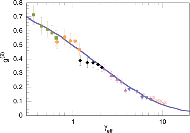
Figure 15. Measurement of the local two-body pair correlation, using photoassociation data and comparison with exact predictions from the Lieb–Liniger model for the ground state. γeff is the effective interaction parameter, that takes into account the inhomogeneity of linear densities across the cloud. Reprinted figure with permission from (Kinoshita et al 2005), Copyright 2015 by the American Physical Society.
Download figure:
Standard image High-resolution imageThe experiment of Kinoshita et al (2005) is realized in a 2D optical lattice, so that a 2D array of 1D inhomogeneous tubes is populated. More precisely, the atom density varies within each tube because of the harmonic longitudinal confinement V(x), and the atom number N per tube varies among the tubes. The data analysis uses the LDA. The local loss rate is proportional to the local value of n2
g(2)(0), where g(2)(0) depends on n via its dependence on the interaction parameter γ = mg/(ℏ2
n):  . One assumes that
  is linear in log(γ), which is a good approximation for the data range explored (see figure 15). Then the loss rate is expected to be proportional to
  , where
  is the mean linear density seen by atoms and γeff is such that log(γeff) is the spatial average of log(γ), weighted by n2. To evaluate γeff and
  , the distribution of atoms among the tubes is assumed to be that corresponding to the initial shape of the 3D BEC, and, within a 1D tube, the Lieb–Liniger equation of state is used. Finally, the value of
  deduced from experimental data is shown in figure 15. It is in remarkable agreement with the prediction from the Lieb–Liniger model. The data show the crossover between the quasicondensate regime, where g(2)(0) ≃ 1, as in a true BEC, and the hard-core regime, where g(2)(0) ≪ 1, as for a Fermi gas.
Shortly before that measurement of g(2)(0), the observation of 1D Bose gases in the hard-core regime had been achieved by Kinoshita et al (2004), who measured the total energy of an array of 1D gases by 1D expansion, as well as the length of the trapped atom clouds. The approach to the hard-core regime was also signaled by a measured reduction of the three-body loss rate (Tolra et al 2004) (see section 5 for a discussion of three-body losses).
3.2.2. Analysis of density profiles: Yang–Yang thermodynamics
Remarkably, the results for g(2)(0) briefly reviewed in the previous subsection are in good agreement with the theoretical prediction for the ground state of the 1D Bose gas. However, in many experimental situations, the gas is not in its ground state. As reviewed in subsection 1.6, exact theory results from Yang and Yang (1969) are available for thermodynamic quantities at thermal equilibrium. In several experimental works, the data were found to be in very good agreement with predictions from Yang–Yang thermodynamics.
The first comparison between experiments and the finite-temperature thermodynamics of Yang and Yang was done by van Amerongen et al (2008), who analyzed the density profiles of trapped 1D gases. This work used an atom chip setup: atoms are confined in magnetic traps realized by microwires deposited on a chip. In contrast with optical trapping, a single 1D cloud is observed, which allows a more direct comparison with theoretical predictions, since no averaging over tubes is required. This permits investigation of the density profile of the 1D gas, confined in a longitudinal potential V(x). As discussed in subsection 3.1.3, the longitudinal trapping is weak enough that the LDA is valid. For a gas at thermal equilibrium, the LDA means that the gas at position x is described by a gas at temperature T and chemical potential μ(x) = μ0 − V(x). Thus, the density at position x is

where nYY(T, μ) is the linear density of the homogeneous Lieb–Liniger gas at temperature T and chemical potential μ, referred to as the Yang–Yang equation of state. Thus, if V(x) is known, the experimental density profile can be compared to the theoretical curve, with two adjustable parameters: the temperature T and the chemical potential μ0. In the experiment of van Amerongen et al (2008), however, the population of transversely excited states was not negligible. This was taken into account in the theoretical model by treating each transversely excited state as an ideal 1D Bose gas, at thermal equilibrium with the 1D gas in the transverse ground state. This treatment results in a modified Yang–Yang equation of state n(T, μ). Figure 16 reproduces the experimental density profiles of van Amerongen et al (2008) compared with the theoretical curves of the modified Yang–Yang equation of state, with μ0 and T as fitting parameters. The theoretical curves reproduce the measured profiles very well.
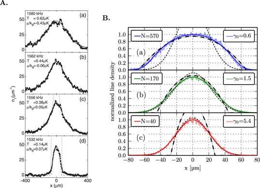
Figure 16. Density profiles of 1D gases, fitted with thermal equilibrium density profiles. The latter are computed, knowing the longitudinal potential, using the Yang–Yang equation of state (Yang and Yang 1969), and assuming an LDA. (A) Measured density profiles (black circles), compared to Yang–Yang profiles (solid lines). Transversely excited states are taken into account as ideal Bose gases. Reprinted figure with permission from (Yang and Yang 1969), Copyright 1969 by the American Physical Society. (B) Density profiles for different 1D gases, located at different positions in an array of 1D tubes. They are obtained from the raw data, which include a column integration of the signal, using an Abel transformation. The Yang–Yang fit is shown as a solid smooth line. Reprinted figure with permission from (Vogler et al 2013), Copyright 2013 by the American Physical Society.
Download figure:
Standard image High-resolution imageSince these pioneering results, the analysis of density profiles of 1D gases using the Yang–Yang equation of state has been realized successfully in other experiments (Armijo et al 2011, Vogler et al 2013). In (Vogler et al 2013) the experimental setup uses an optical lattice, and density profiles are acquired using an electron beam propagating perpendicularly to the longitudinal direction x. The resolution attained using electron-beam imaging is sufficiently good to resolve individual 1D tubes. However, the data analysis is complicated by the fact that column-integrated density profiles are acquired, the integration being done over the direction of propagation of the electron beam. Thus, the raw data mix information about different 1D tubes that have different density profiles. The density profile of individual 1D tubes can, however, be extracted deconvoluting for the effect of the column integration, if one assumes invariance by rotation of the tubes’ distribution. The deconvolution technique, that does not require an a priori knowledge of the tube distribution, uses the Abel transformation. The resulting density profiles of individual 1D gases, shown in figure 16, fit remarkably well with the Yang–Yang theory.
3.2.3. Density fluctuations
A more stringent test of Yang–Yang thermodynamics can be made if one investigates not the density profile but its fluctuations. For this purpose, one can investigate the atom-number fluctuations in a pixel whose size Δ is much smaller than the length of the cloud, and much larger than the correlation length of the gas. We note the atom-number fluctuations in a pixel δN = N − ⟨N⟩, where N is the atom number in the pixel.
Then, if one assumes thermal equilibrium, the gas contained in the pixel can be described by a Gibbs ensemble, the rest of the cloud acting as a reservoir of energy and particles. Then atom-number fluctuations fulfill, for any integer K,

where n(μ, T) is the equation of state of the gas. Thus, the measured density fluctuations can be compared to expectation values derived from the Yang–Yang equation of state. Notice that, in contrast with the experiments presented above, no precise knowledge of the longitudinal potential V(x) is required. The longitudinal potential is irrelevant in the data analysis: it is simply useful to sample different densities at a given temperature.
In order to measure density fluctuations, ensemble measurements, such as those realized in setups using 2D optical lattices, are prohibited. Thus, such measurements have been realized only in an atom chip setup. To extract density fluctuations, one records an ensemble of density profiles, all taken with identical experimental parameters, from which a statistical analysis is performed. Measurements of density fluctuations in 1D gases were first performed in (Esteve et al 2006). Comparison with Yang–Yang predictions were performed in (Armijo et al 2011, 2010, Jacqmin et al 2011). In (Armijo et al 2011), the dimensional crossover from 3D to 1D was investigated, and it was shown that it is well accounted for by the aforementioned modified Yang–Yang equation of state, which includes the effect of transversely excited states treated as ideal Bose gases. Figure 17 displays a selection of results from the two latter references.
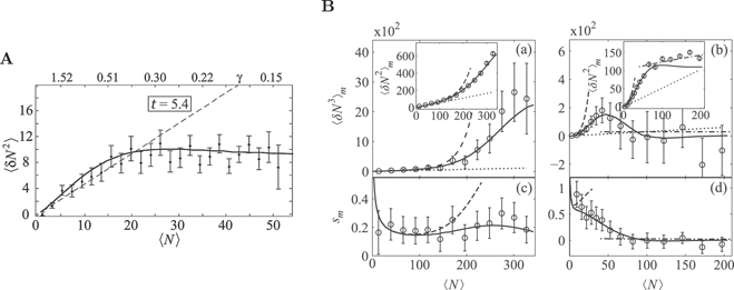
Figure 17. Density fluctuations in 1D Bose gases, compared to Yang–Yang predictions (see equation (107)). (A) Dots: measured density fluctuations. Solid line: Yang–Yang predictions. The reduced temperature t is t = 2ℏ2
kB
T/(mg2). The dashed line shows the shot noise limit, whose amplitude is reduced because of the smearing produced by the finite optical resolution. The fact that gas never shows super-Poissonian fluctuations, that would be associated with bosonic bunching, signals the entrance into the strongly interacting regime. ⟨N⟩ = nΔ where n is the linear density and Δ the pixel size, equal to 4.5 μm. Reprinted figure with permission from (Jacqmin et al
2011), Copyright 2011 by the American Physical Society. (B) Third moment of the density fluctuations. Solid lines show the Yang–Yang prediction, with transversely excited states considered as ideal Bose gases. The dotted line gives the shot noise level, corrected for the effect of finite resolution. The dashed lines show the predictions for an ideal Bose gas. Graphs (c) and (d) show the skewness of the atom-number distribution, defined as  . In the inset of graph (b), the deviation of the measured ⟨δN2⟩ to the Yang–Yang prediction (solid line), is due to the swelling of the transverse wavefunction, which occurs because the condition μ ≪ ω⊥ is not fulfilled. This 3D effect is taken into account in the quasicondensate predictions shown as dotted-dashed lines. Reprinted figure with permission from (Armijo et al
2010), Copyright 2013 by the American Physical Society.
. In the inset of graph (b), the deviation of the measured ⟨δN2⟩ to the Yang–Yang prediction (solid line), is due to the swelling of the transverse wavefunction, which occurs because the condition μ ≪ ω⊥ is not fulfilled. This 3D effect is taken into account in the quasicondensate predictions shown as dotted-dashed lines. Reprinted figure with permission from (Armijo et al
2010), Copyright 2013 by the American Physical Society.
Download figure:
Standard image High-resolution image3.2.4. Techniques for measuring the momentum distribution
While all the above results concern observables that involve only the real-space density, information is also contained in other observables, in particular the momentum distribution. The momentum distribution has been measured in several experiments using different techniques, which we briefly review now.
The first technique that was used was the so-called Bragg technique. The idea is to shine two laser fields with wavevector difference q and frequency difference ω onto the atomic cloud. The action on the cloud is described by the addition of a new term to the Hamiltonian, which reads

where each term corresponds to the absorption of a photon in one laser beam and stimulated emission in the other, a process called a Bragg process. For counterpropagating lasers, q is usually very large compared to the typical momentum width of the cloud, and ℏ2 q2/m is typically much larger than the energy per atom. In this case, called the Doppler regime, the atom promoted to the momentum state k + q by the Bragg process can be considered as effectively removed from the system, and the final energy is about ℏ2(k + q)2/(2m) ≃ Erec + ℏ2 kq/m, where Erec = ℏ2 q2/m is the recoil energy, and the second term is the Doppler shift. Then the Fermi golden rule leads to a rate of Bragg transfer Γ which obeys

where conservation of energy imposes k = m(ℏω − Erec)/(ℏ2 q). Thus, measuring the loss rate of the atomic cloud as a function of the Bragg detuning ω gives access to the momentum distribution of the atoms. The energy deposited in the system per unit time is nothing but Γℏω, such that one can equivalently deduce the momentum distribution from the measurement of the energy increase rate versus ω. Note that, by choosing ω close to N2 Erec, where N is an integer, one can induce Nth-order Bragg processes: the momentum transfer is then Nq, which allows deeper access inside the Doppler regime. This technique was first used in (Stenger et al 1999) in a 3D BEC, where it confirmed the presence of long-range order in the cloud. Applied to a very elongated BEC, it was used to demonstrate the presence of longitudinal thermally excited phase fluctuations (Richard et al 2003). More recently, it was implemented in 1D gases realized in a 2D optical lattice (Fabbri et al 2011). Note that, going beyond the Doppler limit of large momentum transfer, the Bragg techniques allow the measurement of the dynamic structure factor. Such measurements have been compared to results based on the Lieb–Liniger model in (Fabbri et al 2015) and (Meinert et al 2015).
Bragg momentum spectroscopy suffers from low signal amplitude, since it is based on a perturbative analysis, and, most importantly, it does not allow recording of the whole momentum distribution in a single measurement. This impedes the measurement of correlations in momentum space. We now discuss another technique that enables the recording of the whole momentum distribution of 1D gases in a single measurement. The key point is to be able to switch off the interactions almost instantaneously with respect to the longitudinal motion. This can be achieved, close to Feshbach resonances, by manipulating the interaction strength with a magnetic field (Stewart et al 2010). However, in the special case of 1D gases, this switch-off can be achieved very easily by removing the transverse confinement: after the switch-off of the transverse potential, the transverse wavefunction expands in a typical time of the order of 1/ω⊥, much shorter than typical times associated with the longitudinal motion, and this amounts to an almost instantaneous vanishing of the effective 1D interaction strength with respect to the longitudinal motion.
Once interactions have been effectively switched off, one is left with the task of measuring the momentum distribution of an ideal gas. This could be done by a simple ballistic expansion, following the sudden switch-off of the longitudinal potential: after an expansion time long enough that the final cloud size is much larger than its initial size, the density distribution becomes homothetic to the momentum distribution. This technique, usually referred to as the time-of-flight technique, is used for instance in (Fabbri et al 2011) and (Malvania et al 2021, Wilson et al 2020). However, in experiments using very long initial clouds and/or gases lying deep in the quasicondensate regime, such as atom chip experiments, this technique typically requires unrealistic expansion times. To overcome this difficulty, one can use the so-called focusing method. This method, first implemented in (Shvarchuck et al 2002), consists of applying a short pulse of a strong longitudinal harmonic potential. Atoms do not have time to move during this pulse, but they acquire a momentum kick δp = −Ax proportional to their distance x from the center. The cloud then undergoes free evolution. After a time equal to the focusing time tf = m/A, the density distribution is homothetic to the initial momentum distribution. This technique effectively erases the information on the initial cloud longitudinal spread.
3.2.5. Results in momentum space
All measurements reviewed in subsections 3.2.1–3.2.3 probe thermodynamic quantities. On the theory side, those are easily accessible numerically using Yang–Yang thermodynamics for thermal equilibrium states. In contrast, the momentum distribution is not a thermodynamic quantity.
The momentum distribution of 1D gases lying in the quasicondensate regime was measured using Bragg spectroscopy by Fabbri et al (2011). The authors show that the measured momentum distribution is close to a Lorentzian. A Lorentzian shape of full-width at half-maximum mkB T/(ℏ2 n) is expected for homogeneous gases in this regime, for wavevectors lying in the phononic regime (Jacqmin et al 2012). Within the LDA, the total momentum distribution n(p) is obtained by summing the contributions of each small fluid cell. For a harmonically confined quasicondensate, one finds a momentum distribution that stays very close to a Lorentzian (Jacqmin et al 2012).
The focusing method was used for 1D gases trapped on an atom chip in (Davis et al 2012). The measured momentum distribution n(p) was compared to improved classical field calculations, expected to be valid in the quasicondensate and ideal Bose gas regimes. The transversely excited states cannot be neglected in those experiments and they were taken into account assuming they behave as ideal Bose gases. In fact, in this paper, the authors propose a thermometry method. More precisely, they evaluate the total kinetic energy EK = ∫n(p)p2/(2m)dp from the measured momentum distribution n(p). EK is a thermodynamic quantity that can be calculated with Yang–Yang thermodynamics, and that can be fitted to extract the temperature. The fact that EK is a thermodynamic quantity follows from the following argument. EK can be computed using the LDA as the integral of the kinetic energy density eK(x) over the cloud. The latter is eK(x) = e(n(x), T) − eint(n(x), T) where e(n, T) is the energy density of the Lieb–Liniger gas at density n and temperature T, and eint(n, T) is its interaction energy. Both are thermodynamic quantities: the interaction energy can be obtained from the Hellmann–Feynman theorem, see equation (75). For data analysis, one adds the contribution of the transversely excited states, considered as ideal Bose gases.
The first comparison between the measured momentum distribution of a 1D Bose gas and exact calculations was done in (Jacqmin et al 2012). The first-order correlation function at thermal equilibrium was computed with a Monte Carlo method, which gave very good agreement with the measured momentum distribution. The measured in situ density fluctuations (subsection 3.2.3) also fitted very well with the temperature fitted from the Monte Carlo simulations. The momentum distribution n(p) was measured across the smooth transition between the ideal Bose gas regime and the quasicondensate regime. No striking modification of n(p) was observed across the transition; in particular, it conserves a Lorentzian-like shape. (We recall that the crossover occurs for a degenerate gas whose momentum distribution, in the ideal gas regime, has a Lorentzian central shape.)
Using the focusing technique, the full momentum distribution of the sample can be recorded in a single measurement. Thus, it is possible not only to extract the mean momentum distribution n(p), but also its fluctuations δnp . In (Fang et al 2016), the correlations ⟨δnp δnp′⟩ are deduced from a statistical analysis of hundreds of images taken in the same experimental conditions. The results are in very good agreement with numerically exact results obtained, for a gas at thermal equilibrium, using a quantum Monte Carlo algorithm, as seen in figure 18. The calculation uses a discretized model and a worm algorithm. The crossover between the ideal Bose gas and the quasicondensate regime has a clear signature in momentum space correlations. The ideal Bose gas regime is characterized by a bunching phenomenon for equal momenta. In the quasicondensate regime, on top of the bunching seen on the diagonal, anti-correlations appear for different momenta. Those anti-correlations ensure small density fluctuations, the latter being inhibited in the quasicondensate regime because of the large interaction energy they would require. The presence of those anti-correlations in the quasicondensate regime was predicted using Bogoliubov theory in (Bouchoule et al 2012).
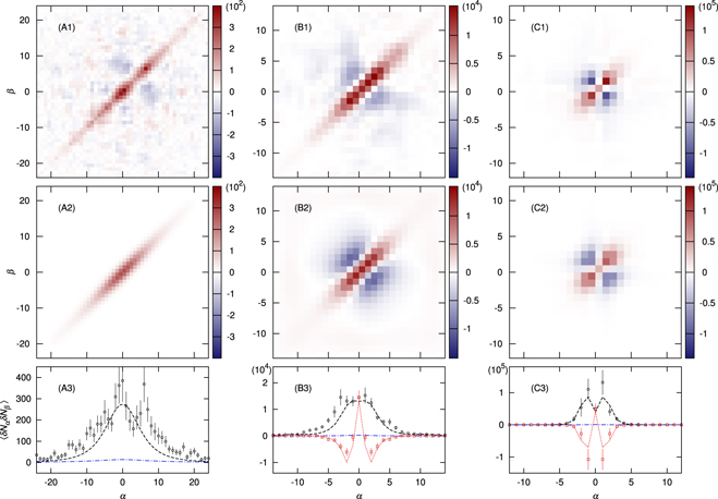
Figure 18. Correlations in momentum space. (A1), (A2), (B1), (B2), (C1) and (C2) show the correlation ⟨δnα δnβ ⟩, where α and β denote the index of the pixel in momentum space (equal to ℏ × 0.15 μm−1). Column A corresponds to a gas in the ideal Bose gas regime; column C to a gas in the quasicondensate regime; and column B to a gas at the crossover between both regimes. Experimental data (first row) are compared to Monte Carlo calculations (second row). (A3), (B3) and (C3) show cuts along the diagonal and the anti-diagonal. Reprinted figure with permission from (Fang et al 2016), Copyright 2016 by the American Physical Society.
Download figure:
Standard image High-resolution image3.2.6. Other higher-order correlation functions
The two-body correlations in momentum space presented in figure 18 are related to the four-point correlation function of the atomic creation/annihilation operator. The four-point correlation function can also be probed by investigating density fluctuations resulting from a short free evolution time. The idea is to switch off the interactions between atoms abruptly, for instance by removing the transverse confinement (subsection 3.2.4), and then to remove the longitudinal confinement and let the gas evolve freely for a short time tfree. In contrast with the time-of-flight method used to measure momentum distribution (subsection 3.2.4), here the free evolution time is assumed to be short, such that the mean density profile of the cloud barely changes. Thus, no information is gained from the mean profile. Instead, one investigates the density fluctuations, also called density ripples. They are characterized by their spectral density ⟨|ρ(q)|2⟩. For wavelengths much shorter than the size of the mean density profile, the latter is related to the four-point correlation function of the atomic field,

where expectation values are taken in the 1D gas before the expansion. For very large q, since there is no long-range order in the 1D gas, the atomic fields at positions separated by qtfree are uncorrelated and the above expression vanishes. On the other hand, for very small q one recovers the spectral density of density fluctuations that were present in the initial gas. This measurement turns out to be particularly relevant in the quasicondensate regime. There, the initial density fluctuations are negligible and ⟨|ρ(q)|2⟩ results from the transformation of phase fluctuations into density fluctuations during the free evolution. Density ripples were first investigated in (Dettmer et al 2001) in a quasi-1D setup. It was then used for thermometry in (Manz et al 2010) in a 1D gas realized in an atom chip setup. For q small enough that ℏqtfree/m is very small compared to the correlation length of the phase fluctuations, one finds from equation (110) that the power spectrum of density fluctuations after free evolution during tfree is simply proportional to the power spectrum of the initial phase fluctuations at the same wavevector. Thus, the analysis of density ripples allows one to access each Bogoliubov mode individually. This feature was used in (Schemmer et al 2018) to monitor the dynamics produced by an interaction quench. Finally, let us stress that the measurement of density ripples is clearly very different from the measurement of the momentum distribution, as the momentum distribution n(p) mixes all Bogoliubov modes.
3.2.7. Validity of the thermodynamic equilibrium
In the experiments reviewed so far, the 1D gases were shown to present behavior in very good agreement with that of a gas at thermal equilibrium. However, as discussed in section 1.6, the 1D Bose gas is integrable so there is no reason to assume that isolated 1D gases should be described by thermal equilibrium states. Instead, it is expected that the local state of the gas is a GGE characterized by its rapidity distribution. The rapidity distribution should depend on the preparation scheme of the gas. In particular, as discussed below in section 5, losses are expected to bring the system into a state that is not a thermal state. Since losses are usually present, at least in the preparation stage, one expects the state to lie in a non-thermal state.
The reason why the above data are in good agreement with thermal equilibrium predictions is unclear. It may be due to the integrability breaking produced by populated transversely excited states (Li et al 2020, Møller et al 2021). The population of transversely excited states decreases exponentially with the ratio between the mean energy per atom and ℏω⊥, the gap between the transverse ground state and the transversely excited states. This population can be totally negligible for gases deep enough into the 1D regime. However, three-body processes involving a virtual excitation of transversely excited states are still expected to lead to integrability breaking (Mazets 2011a, Mazets et al 2008, Tan et al 2010). On long time scales, the longitudinal potential is also expected to break the integrability and to bring the cloud toward a thermal state. This effect was first pointed out in (Mazets 2011b), within a semi-classical approach taking into account the Wigner time delay associated with the two-body collision. Using an improved GHD approach that includes diffusive terms, the relaxation toward a thermal equilibrium in the presence of an external potential was recently computed in (Bastianello et al 2020a), see figure 12.
In contrast with the results presented so far, there do exist experimental data that show the presence of long-lived non-thermal states. In (Langen et al 2015), a 1D gas in the quasicondensate regime is cut into two 1D gases by transverse splitting, and the evolution of the relative phase between the two clouds θ1(x, t) − θ2(x, t) is monitored. Within a Bogoliubov analysis, the anti-symmetric degrees of freedom are decoupled from the symmetric ones and their Hamiltonian is a simple integrable model which reduces to a collection of independent modes. Within Bogoliubov theory, the GGE is simply parameterized by the population of each Bogoliubov mode, or equivalently by its temperature. Only large-scale variations are probed in (Langen et al 2015), which belong to the phononic regime. For a rapid splitting process, all anti-symmetric phononic modes are expected to share the same temperature (Gring et al 2012), so one should recover a thermal ensemble. However, for another splitting procedure, the experimental results show that all Bogoliubov modes do not share a common temperature, so that one has a true GGE. The GGE realized in this experiment is a GGE relative to the Bogoliubov model; it is not a GGE of the Lieb–Liniger gas. On longer time scales, coupling between the Bogoliubov modes is expected to lead to the relaxation of this GGE toward a thermal ensemble for the phononic modes (Mazets and Schmiedmayer 2009).
In (Johnson et al 2017), a single 1D gas lying in the quasicondensate regime is investigated. Long-lived non-thermal states are reported with a mode occupation of the phononic modes corresponding to some temperature. This temperature is shown to be incompatible with the population of the short-wavelength collective modes. It is proposed that such a non-thermal state emerges from the effect of atom losses. Such non-thermal states are robust with respect to the trivial Bogoliubov dynamics, however the Bogoliubov modes are not the real infinite-lifetime quasiparticles of the Lieb–Liniger model. There is no one-to-one correspondence between the population of the Bogoliubov modes and the rapidity distribution. Yet, the short-wavelength Bogoliubov modes should correspond to high rapidities, while the phonons should be related to small deformations of the rapidity distribution near its zero-temperature edges. Thus, one expects that the non-thermal states reported in (Johnson et al 2017) are really robust against the Lieb–Liniger Hamiltonian, which means that they correspond to non-thermal rapidity distributions.
Finally, let us also mention that the most striking long-lived non-thermal state realized in a 1D Bose gas was reported as early as 2006 in the Newton cradle experiment (Kinoshita et al 2006). This work is reviewed in detail in section 4.1.
Although long-lived non-thermal states have been reported, integrability breaking mechanisms, such as the effect of transversely excited states in virtual processes (Mazets 2011b) or the effect of longitudinal potential (Bastianello et al 2020a), are expected to bring the system toward a thermal equilibrium state described by the Gibbs ensemble at very long time. Note, however that loss mechanisms, whose effects are discussed in section 5, might prevent the observation of thermalization.
3.3. Measurement of the rapidity distribution
As explained in section 1.2, rapidities are the asymptotic momenta of the atoms after a 1D expansion. This characterization can be viewed as the definition of the rapidities. It also shows that the rapidity distribution is an observable. Owing to the important role of the rapidity distribution, the experimental ability to measure it is a key development for the study of 1D gases.
The first experimental measurement of the rapidity distribution was done by Wilson et al (2020), for gases lying quite deep inside the hard-core regime. In this experiment the trapping potential is the sum of a 2D array of 1D tubes realized by a 2D optical lattice, and a slowly varying trapping potential, which provides a longitudinal confinement along the tubes. Removing the slowly varying potential, a 1D expansion is performed within each tube. After a sufficiently long expansion time, the momentum distribution converges toward the rapidity distribution. The momentum distribution is then measured using the time-of-flight technique, performed by suddenly turning off all confining potentials (including both the 1D longitudinal confinement and the 2D array of tubes). Interactions are effectively almost instantaneously turned off by the rapid transverse expansion of each tube. Thus, the cloud performs a ballistic expansion such that, at long time, the density profile reflects the momentum distribution.
The momentum distribution measured for different 1D expansion times is found to be in very good agreement with theoretical predictions, see figure 19 from (Wilson et al 2020). The calculation of the evolution during the 1D expansion assumes hard-core bosons and is done for a gas initially in the ground state. For long enough expansion times, the momentum distribution converges toward the rapidity distribution.
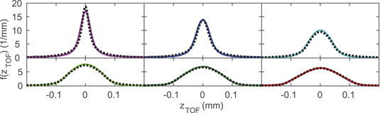
Figure 19. Measurement of the rapidity distribution. Density profiles recorded after a 1D expansion during a time texp, followed by a ballistic (free) expansion during tfree. texp is equal to (from left to right and top to bottom) 0, 1, 3, 6, 9, 12 ms and tfree = 70 ms −texp. Experimental data (solid lines) are in remarkable agreement with theoretical predictions for hard-core bosons (dashed lines). For long 1D expansion times, the momentum distribution converges toward the rapidity distribution. From (Wilson et al 2020). Reprinted with permission from AAAS.
Download figure:
Standard image High-resolution image4. Experimental tests of GHD
GHD is an effective theory which assumes separation of scales, i.e. long wavelength and slow dynamics, see figure 6. It is an approximate theory, and testing it experimentally is highly desirable to establish its relevance for the description of 1D Bose gases. The results reviewed in section 3 show that the Lieb–Liniger model is realized experimentally in cold atom experiments. On intermediate time scales, small enough that unavoidable integrability breaking mechanisms, such as the effect of transversely excited states (Mazets 2011b), have negligible effects, but long compared to the relaxation time of the Lieb–Liniger model, one expects to be able to perform experimental tests of GHD. This has been done in two cold atom experiments up to now. The first one investigates a weakly interacting 1D gas in an atom chip setup. The second one uses strongly interacting atoms and investigates arrays of 1D gases. In both cases, an out-of-equilibrium situation is produced by a quench of the longitudinal potential and the subsequent time evolution is recorded.
Before we present those experimental tests of GHD, we briefly discuss the quantum Newton cradle experiment (Kinoshita et al 2006), which was performed a decade before the advent of GHD, and served as major motivation for many theoretical developments that occurred during that time. The questions raised by that pioneering experiment have driven the research on the out-of-equilibrium dynamics of integrable quantum systems, including the development of GHD.
4.1. The quantum Newton cradle experiment
In their famous experiment on non-equilibrium dynamics in a 1D Bose gas, Kinoshita et al (2006) use an array of 1D tubes, in a blue-detuned 2D optical lattice setup, with a longitudinal confinement, approximately harmonic, realized by an additional smooth dipole trap. The interaction parameter γ (see equation (7)) at the center of the trap, averaged over the collection of 1D gases, ranges from 0.6 to 4, depending on the data set.
An out-of-equilibrium initial situation is realized by applying two Bragg pulses on the cloud, such that the zero-momentum state is mostly transferred to a superposition of the two momentum states p = ±2ℏk. (Because of the interactions between atoms, that momentum transfer is not perfect; for a theoretical study of the state generated by the Bragg pulse, see (van den Berg et al 2016).) The cloud then evolves freely inside the trap up to time t. At time t, the longitudinal potential is turned off and atoms undergo a 1D expansion during an expansion time texp., large enough so that the final size of the atomic cloud is much larger than its initial size. After the 1D expansion, an image is recorded. The image performs a column integration in a direction perpendicular to the longitudinal direction. Figure 20 shows such images, for different evolution times t that span an oscillation period of the longitudinal potential: τ = (2π)/ω∥, where ω∥ is the frequency of the longitudinal potential. At t = 0, one observes two well-separated clouds, corresponding to the two components of different momenta created by the Bragg pulses. Then, one sees a dynamics resembling that which would be found if the atoms were non-interacting. In particular, at time τ/2, one recovers a situation close to the initial one: roughly speaking, the ‘cloud’ of initial momentum 2ℏk has performed half an oscillation in the harmonic trap and its momentum is now −2ℏk.
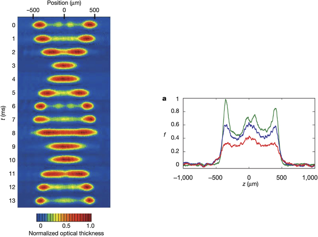
Figure 20. Quantum Newton cradle experiment. Two ‘clouds’ at different mean momenta are prepared by Bragg pulses. (Left) Absorption images of the cloud after an evolution time t in the longitudinal potential, followed by a 1D expansion during a given time texp. The period of the dipole motion in the longitudinal harmonic trap is spanned: 13 ms = τ = (2π)/ωz . (Right) Longitudinal density profiles. The green line is the profile averaged over the first oscillating period. For times t > 10τ, the longitudinal profile barely changes during an oscillation period, as expected because of dephasing induced by the spread of ωz among the 1D tubes. Blue and red lines show the profiles at t = 15τ and t = 30τ. One observes a decrease of the total atom number, due to the three-body recombination effect. The shape of the distribution, however, barely changes and does not converge toward the shape of a thermal equilibrium state. Reprinted by permission from Springer Nature Customer Service Centre GmbH: Nature (Kinoshita et al 2006).
Download figure:
Standard image High-resolution imageAfter an evolution of about 10τ the images show small variations on an oscillation period. This is consistent with the dephasing effect due to the spreading of ω∥ among the 1D tubes. A slow time evolution of the longitudinal profile is observed, see figure 20. This slow evolution is attributed to atom losses and to a small heating rate. Importantly, the measured longitudinal distribution does not evolve toward a thermal equilibrium distribution, at least not on the time scale probed in the experiment.
Theoretical modeling of this experiment is easy only in two asymptotic regimes: the ideal Bose gas regime, and the hard-core regime. In both cases, the dynamics is that of a non-interacting gas, see subsection 1.8. In those limits, one expects to observe undamped oscillations going on for ever, for a single 1D tube and a purely harmonic trap. The data of Kinoshita et al (2006) are compatible with this interpretation: at short times, the evolution is close to that of an ideal gas, and at longer times the observed damping can be attributed to dephasing between 1D gases. At very long times the evolution can be attributed to atom losses. The observed behavior is thus qualitatively similar to that expected for hard-core bosons, and this is because γ is sufficiently large so the 1D gases are quite well inside the hard-core regime. However, a quantitatively accurate modeling of those results, properly taking into account the finite value of γ, was completely out of reach at the time when (Kinoshita et al 2006) was published. In the decade that followed the experiment, no theory was capable of simulating it, taking into account the finite value of the interaction strength.
GHD is the first and, until now, only theory capable of obtaining quantitative predictions for such an experiment, valid for any initial situation (see section 2.2). This illustrates the power of that theory. The physical picture, detailed in section 2.2, is summarized below. The time evolution of the rapidity density ρ(x, θ) develops sharp structures due to the trap anharmonicity (Caux et al 2019). At some point those structures will be so narrow that the large-scale approximation of Euler-scale GHD will fail. One then expects the fine structures to disappear and the rapidity distribution to tend to a rapidity distribution that is a stationary solution of the GHD equations and that is non-thermal (Cao et al 2018, Caux et al 2019). On even longer time scales, under the combined effects of the integrability breaking produced by the longitudinal potential and diffusive terms, which are beyond Euler-scale GHD, the system will eventually drift toward a thermal equilibrium state (Bastianello et al 2020a). Relaxation toward a thermal equilibrium state has also been observed in classical field numerical simulations of the Newton cradle setup (Thomas et al 2021). The classical field, which is expected to describe weakly interacting gases with large mode population (see section 1.8.5), is not restricted to the description of long-wavelength behavior: it is beyond Euler-scale GHD, and this explains why it can lead to thermalization in the presence of an external potential.
In the quantum Newton cradle experiment, effects that are beyond pure 1D physics may also play a role. The population of transversely excited states is negligible since ℏω⊥ (i.e. the energy gap between the transverse ground state and the first excited state) greatly exceeds the typical longitudinal energy per atom. In particular, thanks to the use of blue-detuned lasers for the realization of the 2D lattice, the potential depth, limited by longitudinal trapping, is smaller than ℏω⊥, which ensures that the longitudinal energy stays smaller than ℏω⊥. However, even when they are not populated, transversely excited states can contribute as virtual states in three-body processes (Mazets et al 2008). This phenomenon introduces an effective three-body interaction that breaks the integrability of the Lieb–Liniger model, and it might contribute significantly to the relaxation toward a thermal equilibrium.
Similar quantum Newton cradle experiments have been reproduced in (Li et al 2020, Schemmer et al 2019, Tang et al 2018). Li et al (2020) studied the effect of integrability breaking due to the presence of atoms in transversely excited states, while Tang et al (2018) investigated the effects of dipolar interactions.
4.2. Test of GHD in an atom chip setup
A first experimental demonstration of the validity and relevance of GHD was carried out by Schemmer et al (2019). In this experiment, a 1D gas is realized on an atom chip. The initial cloud is at equilibrium in a regime close to the quasicondensate regime. Dynamics is initiated by a quench of the longitudinal potential, and the time evolution of the density profiles is recorded. For all situations considered, the results are in very good agreement with the predictions of the GHD theory.
The data are also compared to predictions of standard hydrodynamics, given by the Euler equations (3) of the introduction (see also subsection 2.1). In contrast with GHD, this standard hydrodynamic approach assumes that the gas is locally at thermal equilibrium. The numerical solution of the Euler equations involves the numerically tabulated pressure  which is obtained from the Yang–Yang equation at thermal equilibrium, see subsection 1.6. A clear failure of standard hydrodynamics is found when the 1D gas is prepared at equilibrium in a double-well potential, and the double well is suddenly switched off and the gas is allowed to expand freely in 1D. In that case, the predictions of standard hydrodynamics differ strongly from those of GHD. Figure 21 shows the experimental data, together with GHD calculations and standard hydrodynamics calculations. The experiment clearly discriminates between both theories, and the data are found to be in agreement with GHD but not with standard hydrodynamics.
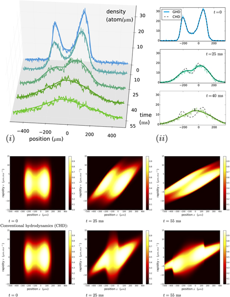
Figure 21. (Top) Experimental test of GHD theory. Shown are density profiles after a quench from a double-well potential to a flat potential. The experimental data (noisy curves) are in very good agreement with GHD predictions (smooth solid lines). The standard hydrodynamics (dashed lines on the right figures) fails to capture the physics. Reprinted figure with permission from (Schemmer et al 2019), Copyright 2019 by the American Physical Society. (Bottom) Calculations of the expected rapidity distributions after a release from a double-well potential. The figures show the evolution of the Fermi occupation ratio ν(x, θ), which is in one-to-one correspondence with the rapidity distribution ρ(x, θ) (see subsection 1.5). The top row shows the prediction from GHD theory, and the bottom row shows the prediction from standard Euler hydrodynamics. The GHD predicts the appearance of a double-peaked rapidity distribution around the center of the cloud (clearly visible on the plot at t = 55 ms). Standard Euler hydrodynamics, on the other hand, assumes that at each point x the rapidity distribution ρ(x, θ) is the one at thermal equilibrium, which is a single-peaked function. This theory is thus unable to capture the correct physics. Reprinted figure with permission from (Schemmer et al 2019), Copyright 2019 by the American Physical Society.
Download figure:
Standard image High-resolution imageThe origin of the failure of standard hydrodynamics in the above scenario is revealed by the following simple picture (figure 21, bottom). During the time evolution, the two clouds that were initially in each of the potential wells spread, the negative rapidities moving to the left and the positive ones to the right. After some expansion time, at the central position, the positive rapidities from the left cloud meet negative rapidities coming from the right cloud. The resulting rapidity distribution is then double-peaked. The standard hydrodynamic theory cannot capture this feature, because it assumes local thermal equilibrium and the rapidity distribution of thermal states are single-peaked. This striking difference between GHD and conventional Euler hydrodynamics is clearly visible in figure 21, where the calculated Fermi occupation ratio ν(x, θ) is displayed for both theories.
The Newton cradle scenario has also been reproduced in (Schemmer et al 2019), by quenching the longitudinal potential from a double-well to a harmonic potential, see figure 22. One then initiates a dynamics similar to that studied in (Kinoshita et al 2006), with two clouds that oscillate and collide in a harmonic potential. The experimental results compare well with the prediction from GHD. For this scenario, conventional Euler hydrodynamics completely fails: it predicts the formation of a very sharp structure in the density distribution, corresponding to a large gradient of the density, that eventually leads to a shock, at times as small as about 30 ms. The agreement between experimental data and GHD is less good than for the scenario of figure 21. One of the reasons for this might be the effect of three-body losses. In the Newton cradle scenario, large peak densities are attained when both clouds superpose, and the three-body recombination process occurs, leading to atom losses. We find experimentally that the total atom number decreases by about 15% on the time evolution shown in figure 22.
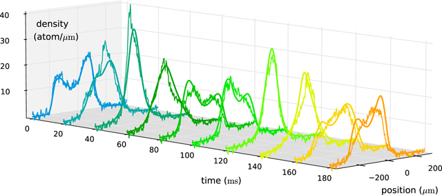
Figure 22. Dynamics induced by a quench from a double-well potential to a harmonic potential, which realizes a situation similar to the quantum Newton cradle. Experimental data (noisy lines) are compared to GHD calculations (smooth solid lines). Because of atom losses, the number of atoms drops by approximately 15% from t = 0 to t = 180 ms. This is not taken into account in the GHD theory. Reprinted figure with permission from (Schemmer et al 2019), Copyright 2019 by the American Physical Society.
Download figure:
Standard image High-resolution image4.3. Test of GHD in strongly interacting gases
In the experiment of Schemmer et al (2019), GHD is tested in a very large atom cloud that contains thousands of atoms, whose longitudinal size, of the order of 100 μm, is very large compared to microscopic scales. In these conditions, GHD is clearly expected to be valid. In a more recent experiment by Malvania et al (2021), GHD is tested in a setup that uses a 2D lattice of 1D gases. In this experiment, the typical atom number N is as low as ten to 20 per 1D gas. Moreover, the (quasi-)harmonic longitudinal potential V(x) can be quenched very dramatically: at time t = 0, the amplitude of the trap can be increased by a factor of as large as 100, so the atom cloud is very strongly compressed. The validity of GHD is severely challenged in this situation, yet the experimental data, which are averaged over all the 1D tubes, are still correctly described by GHD over the first few oscillation cycles. We now discuss the results of Malvania et al (2021) in more detail.
The 1D clouds are prepared from a 3D BEC by adiabatically increasing the depth of the 2D lattice. When the 2D lattice depth is large enough, the gas decouples into independent 1D tubes. The temperature is extremely low, so that each 1D gas is close to the ground state of the Lieb–Liniger Hamiltonian in each tube. The dynamics is generated by suddenly increasing the longitudinal potential V(x) felt by the atoms in each tube. The longitudinal potential V(x), realized using an optical beam, has a Gaussian shape and its depth is increased by a large factor, of ten or 100 depending on the experimental data set. In sharp contrast with (Schemmer et al 2019), the initial cloud lies in the hard-core regime, with mean γ, averaged over the distribution of linear densities, as large as nine. Malvania et al (2021) measure the time evolution of the rapidity distribution (figure 23), using the technique of Wilson et al (2020) reviewed in subsection 3.3. This measurement is a global measurement: the rapidity distribution is integrated over positions x within each tube, and averaged over all the tubes.
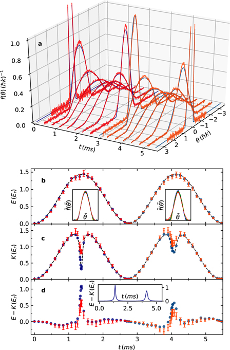
Figure 23. Test of GHD using strongly interacting gases. The dynamics is generated by a sudden increase of the depth of the Gaussian longitudinal confinement by a factor of 100. The first two compression cycles are shown. Experimental data (red curves in (a) and red dots in (b)–(d)) are compared to GHD predictions for a gas initially in the ground state (blue lines in (a)). The blue dots in (b) and (c) are the GHD calculations using the measured atom number at each time, while the dashed line in (b) and (c) is the theory using the average atom number. (a) Measured rapidity distribution f(θ), integrated over positions x and averaged over all 1D tubes, compared to the GHD prediction. (b) Rapidity energy E, i.e. ∫dθ f(θ)(θ2/(2m)), in units of the recoil energy Er. (c) Evolution of the kinetic energy, obtained from the measured momentum distribution w(p): K = ∫dp w(p)(p2/(2m)) (to prevent confusion with notations used in section 5, K is noted as EK in the main text). (d) Interaction energy E − K. From (Malvania et al 2020). Reprinted with permission from AAAS.
Download figure:
Standard image High-resolution imageThe results are shown in figure 23, for a quench of the 1D trap amplitude by a factor of 100. They are in excellent agreement with GHD predictions, which use the Lieb–Liniger ground state within the LDA as the initial state and the zero-entropy GHD equation (88) discussed in subsection 2.3 for the time evolution (figure 24). In the theoretical calculation it is found that, for an increase of the trap depth of the quasi-harmonic (Gaussian) potential by a factor of 100, the dimensionless repulsion strength γ, taken to be initially of order one in the center of the cloud, drops to a value of order 0.1 at the maximum of the compression: the variation of γ as a function of position and time over one compression cycle is very large. In this setup, the contour Γt (see discussion in subsection 2.3 and the caption of figure 24) gets deformed very quickly. Already in the first compression cycle, there are positions in the cloud where the rapidity distribution is no longer that of a thermal equilibrium state. Instead, the local state of the gas consists of a split Fermi sea. The appearance of such exotic rapidity distributions originates both from the non-trivial effect of interactions between atoms—which are stronger at the maximum of the compression, where the atom density is high and the cloud is far from the hard-core regime—and from the anharmonicity of the longitudinal potential. The presence of multiple Fermi seas rules out the possibility of describing the dynamics by standard hydrodynamic approaches (subsection 2.1).
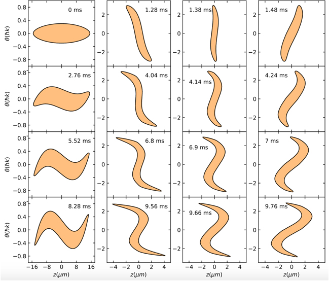
Figure 24. Zero-entropy GHD simulation of a sudden increase of the trap depth of the quasi-harmonic (Gaussian) potential V(x): at t = 0, the depth is increased by a factor of 100, corresponding to the experimental situation of figure 23. Because the gas is initially at zero temperature, the Fermi occupation ν(x, θ, t) is either one (in the orange area) or zero (white area) at any time. The contour Γt (black curve) that separates the two regions evolves according to equation (88). Here the dimensionless repulsion strength γ is initially of order one in the center of the cloud, and it drops to a value of order 0.1 at the maximum of the compression. One clearly sees that the contour Γt gets deformed, as a combined effect of the interactions and of the small trap anharmonicity. Additionally, one observes the appearance of multiple Fermi seas: when a vertical line passing through a point x can intersect the contour Γt at more than two points, the gas is locally in a state known as a ‘split Fermi sea’ (Eliëns 2017, Eliëns and Caux 2016, Fokkema et al 2014). For instance, a double Fermi sea appears near the first compression point (1.38 ms panel). At this point, the conventional hydrodynamic approaches of subsection 2.1 typically fail because of the appearance of shocks, and GHD is necessary to describe the full evolution. From (Malvania et al 2020). Reprinted with permission from AAAS.
Download figure:
Standard image High-resolution imageThe measurement of the rapidity distribution, integrated over the cloud and averaged over all tubes, allows one to monitor the evolution of the rapidity energy. This is defined as E = ∫ρ(x, θ)θ2/(2m)dx dθ for a single 1D cloud, and it is averaged over all clouds in the measurement. The rapidity energy is the total energy, which is conserved, minus the potential energy associated with the confining potential. Since the potential energy oscillates as the cloud breathes, so does the rapidity energy E, as seen in figure 23(b). Moreover, besides the rapidity distribution, Malvania et al (2021) also measure the momentum distribution using a time-of-flight technique (see subsection 3.2.4), from which the kinetic energy EK can be extracted. The time evolution of the kinetic energy is shown in figure 23(c) (notice that EK is simply noted as K in the figure). The difference between the rapidity energy E and the kinetic energy EK is the interaction energy. If the gas remained in the hard-core regime at all times, then one would always have EK = E: the atoms would never be at the same position, so the contact interaction energy would be zero and the rapidity energy would be entirely in the form of kinetic energy. The narrow dip of EK at the time when the cloud is most compressed clearly demonstrates that, at this time, the cloud leaves the hard-core regime. (Notice that it is important that it is the second moment of w(p), i.e. the kinetic energy, that is used as a diagnostic for the departure from the hard-core regime. If, instead, one studied the half-width of w(p), then its evolution would show pronounced dips at the time when the cloud is the most compressed, even if the gas stayed in the hard-core regime throughout the evolution (Atas et al 2017).)
To conclude this section, we stress that the good agreement found by Malvania et al (2021) between experimental data with small atom numbers per tube and the predictions of GHD is a topic that deserves further investigation. As discussed in the supplemental material of (Malvania et al 2021), the averaging over 1D tubes results in a smoothing of small atom number effects, which may explain the good agreement with the hydrodynamic theory to some extent. It would be interesting to investigate the question of the accuracy of GHD for single 1D clouds of a few atoms more systematically. On the theory side, this could be done by performing numerical simulations of a single 1D gas for very small atom numbers (similarly to the numerical results shown in figure 13, but for longer times).
5. Atom losses
When one describes experimental 1D Bose gases by the Lieb–Liniger Hamiltonian (6), one assumes that they are perfectly isolated. However, even the cold atom experiments that realize the best isolated quantum many-body systems are never completely decoupled from their environment. Very often, the main coupling to the environment comes from loss processes in the gas. The purpose of this section is to give an introduction to recent progress on the effect of atom losses in the 1D Bose gas.
We stress that losses break the integrability of the model, so that they may be viewed as one special case of an integrability breaking mechanism—a particularly relevant one, from an experimental viewpoint. For a review of integrability breaking mechanisms in relation to GHD, we refer the reader to the article by Bastianello et al (2021) in this volume.
5.1. Loss mechanisms in experiments
Cold atom gases always suffer from losses. Different mechanisms for losses can be present, which are distinguished by the number of atoms K (K = 1, 2, 3, …) involved in each loss event.
- One-body losses (K = 1) can occur due to collisions with hot atoms from the residual gas in the vacuum chamber. This typically imparts a kinetic energy to the (cold) atoms that is sufficiently large that they leave the trap. One-body losses can also result from de-excitation for atoms lying in a metastable state, spin-flips to an untrapped magnetic state in the case of magnetically trapped atoms (Burrows et al 2017), collisions with energetic electrons (Labouvie et al 2016), or coupling to an untrapped state (Bouchoule and Schemmer 2020, Rauer et al 2016).
- Two-body losses (K = 2) occur, for instance, when atoms are not in their internal ground state and exothermic two-body collisions that change the internal state of the atoms are present (Traverso et al 2009, Yamaguchi et al 2008). The collision residues leave the trap because their internal state is not trapped, or because their kinetic energy exceeds the trap depth. In the presence of a laser, one could also have, starting from two nearby atoms, photoassociation toward excited molecules, which, after de-excitation, produce two very energetic atoms that leave the trap (Kinoshita et al 2005).
- Importantly, cold atom experiments always suffer from three-body losses (K = 3). This is due to three-body recombination, where a deeply bound molecule is formed. The binding energy, typically very large, is released in the form of kinetic energy, and the collision residues leave the trap (Söding et al 1999, Tolra et al 2004).
- In principle, loss processes involving more than three atoms also exist. In particular, losses involving K = 4 atoms have been reported in (Ferlaino et al 2009, Gurian et al 2012).
In the following we consider a general K-body loss process, for a fixed positive integer K. We now explain why the natural theoretical framework to model such a K-body loss process is the Lindblad equation (111) below.
Because the lost atoms can be viewed as escaping toward a reservoir of particles whose state is not being monitored, the atoms remaining in the cloud no longer follow a unitary dynamics. Instead, the density matrix  of the remaining atoms in the gas (not to be confused with the rapidity distribution ρ(θ)) evolves according to a Lindblad equation (see equation (111) below). More precisely, the evolution of the gas under losses is described by a Lindblad equation if one assumes that the dynamics remains Markovian. This assumption holds if the energy width of the reservoir, Eres, which is the energy width spanned by the states of the continuum that are coupled to the trapped atoms by the loss process, is much larger than the energy width involved in the dynamics of the gas. In temporal terms, it corresponds to the fact that the intrinsic duration of the loss event, equal to ℏ/Eres, is much smaller than all other evolution time scales of the gas.
In experiments involving atoms in their internal ground state, the range of the interaction between atoms is typically much smaller than the typical distance between them. Losses can then be modeled by purely local processes: a loss event can occur only when K atoms are found at the same position.
Under these assumptions, the evolution of the density matrix  of a uniform Lieb–Liniger gas of length L under losses is

where H is the Lieb–Liniger Hamiltonian (6). Here Ψ(x)K is the operator that destroys K bosons at position x, and G is a constant characterizing the loss process, with dimensions of lengthK−1 time−1.
5.2. Theory of adiabatic losses
Calculating the evolution of the density matrix  directly from the Lindblad equation (111) for more than a few atoms is, in general, an intractable task. Numerically, the size of the matrix quickly becomes prohibitively large. Therefore, the role of equation (111) is merely to give a formal definition of the theoretical problem one would like to solve. To make progress, further assumptions are needed in order to simplify the description.
In the context of this review of hydrodynamics, where one focuses on effective hydrodynamic descriptions valid at large scales assuming local relaxation, a natural assumption is to consider the limit of adiabatic losses. When the parameter G is small enough that the dynamics induced by losses is much slower than the relaxation time τrelax of the system, the gas always remains in a relaxed state on long time scales. Its local properties are entirely described by the rapidity distribution ρ(θ), and the problem then boils down to computing the time evolution of ρ(θ). To lowest order in the small parameter τrelax GnK−1 (where n = N/L = ∫ρ(θ)dθ is the atom density), the evolution of the rapidity distribution must be of the form

where F[ρ](θ) is some functional of ρ at time t, which needs to be determined from equation (111). The functional F[ρ] has been studied in (Bouchoule et al 2020), which we briefly review now.
The idea is to consider the adiabatic evolution of the conserved local charges Q[f], parameterized by some functions f (see equation (28)). To lighten the notation we simply write ‘Q’ for such a generic charge. Under Lindblad evolution (111), the expectation value of the charge  changes as
 ![$\frac{\mathrm{d}}{\mathrm{d}t}\left\langle Q\right\rangle =G\int \left(\frac{1}{2}\left\langle {{\Psi}}^{{\dagger}K}[Q,{{\Psi}}^{K}]\right\rangle +\frac{1}{2}\left\langle \left[\right.{{\Psi}}^{{\dagger}K},Q{{\Psi}}^{K}\right\rangle \right)\mathrm{d}x$](https://content.cld.iop.org/journals/1742-5468/2022/1/014003/revision6/jstatac3659ieqn157.gif) .
.
Because Q is the integral of a local charge density, Q = ∫q(x)dx, and because ΨK
(x) and Ψ†K
(x) are local operators, the two operators between the brackets are local. Then we know that, after the relaxation time τrelax, their expectation values relax to their values in a GGE, see subsection 1.6. This GGE is a diagonal density matrix which can be characterized by its distribution of rapidities ρ(θ), see subsection 1.6. Using the fact that ![$[{\hat{\rho }}_{\text{GGE}},Q]=0$](https://content.cld.iop.org/journals/1742-5468/2022/1/014003/revision6/jstatac3659ieqn158.gif) , and writing
, and writing ![${\left\langle \mathcal{O}\right\rangle }_{[\rho ]}=\mathrm{t}\mathrm{r}\left({\hat{\rho }}_{\text{GGE}}\mathcal{O}\right)$](https://content.cld.iop.org/journals/1742-5468/2022/1/014003/revision6/jstatac3659ieqn159.gif) for the expectation value of an observable
for the expectation value of an observable  w.r.t. the GGE density matrix parameterized by the rapidity density ρ, we get the evolution equation for the expectation values of the charges

We have used translation invariance, which implies that the integrand is independent of x, to go from the first to the second line.
Equation (113) determines the time evolution of the expectation values of all charges Q under adiabatic losses. We see that the problem of modeling losses boils down to computing the rhs of (113), namely the expectation value in a GGE of an operator of the form Ψ†K (0)[Q, ΨK (0)], where Q is a generic conserved charge, and ΨK (0) is the operator that removes K bosons at the same position.
To connect this simple general result to the evolution of the rapidity distribution (112), we specialize Q to an operator which measures the rapidity distribution. To elaborate, recall that the charges Q[f] (28) are diagonal in the eigenbasis and that their expectation value in a Bethe state  is
is  . Formally, we can consider the charge Q[f] corresponding to the choice f(α) = δ(θ − α), which directly measures the distribution of rapidities ρ(θ). However, to ensure that the charge Q[f] has good locality properties, it is safer to work with a regularization of the Dirac delta function, δσ
, of typical width σ and of total weight ∫δσ
(θ)dθ = 1, which remains a smooth function of θ for any σ > 0 (for example a Gaussian of width σ). Then the choice f(α) = δσ
(α − θ) defines a charge Q[f] = Q[δσ
(. − θ)] which remains sufficiently local so that (113) applies. Thus, we see that the functional F[ρ] entering the evolution equation (112) must be given by
. Formally, we can consider the charge Q[f] corresponding to the choice f(α) = δ(θ − α), which directly measures the distribution of rapidities ρ(θ). However, to ensure that the charge Q[f] has good locality properties, it is safer to work with a regularization of the Dirac delta function, δσ
, of typical width σ and of total weight ∫δσ
(θ)dθ = 1, which remains a smooth function of θ for any σ > 0 (for example a Gaussian of width σ). Then the choice f(α) = δσ
(α − θ) defines a charge Q[f] = Q[δσ
(. − θ)] which remains sufficiently local so that (113) applies. Thus, we see that the functional F[ρ] entering the evolution equation (112) must be given by

It is essentially equivalent to calculating the rhs of (113) for arbitrary charges Q, or to computing the functional F[ρ](θ) defined by (114). Either way, the difficulty lies in computing the expectation value of a specific local operator in a GGE.
Up to now, the following results have been obtained in connection with this problem.
- The functional F[ρ] can been evaluated numerically for a given ρ by performing a Monte Carlo summation over Bethe states (Bouchoule et al 2020), using exact formulas for the matrix elements of ψK (0) between Bethe states, see (Piroli and Calabrese 2015, Pozsgay 2011). The differential equation (112) can then be integrated numerically, see the example shown in figure 25. However, this procedure is numerically heavy: it typically takes a few hours to compute F[ρ] for a given rapidity distribution ρ on a single core (but the procedure can be trivially parallelized).
- The functional F[ρ] is known analytically in the ideal Bose gas regime,and also in the hard-core regime,
 where is the Hilbert transform of the rapidity distribution.The result for the ideal Bose gas is very simple, reflecting the fact that the rapidities are the momenta of the non-interacting bosons in that regime. The combinatorial factor K K! comes from the local K-body correlation (a consequence of Wick’s theorem), and the additional factor K simply comes from the fact that there are K atoms lost in each event.In contrast, the result for the hard-core regime for K = 1 is much more complex, even though it is also related to an underlying model of non-interacting particles, see subsection 1.8. In particular, one sees that F[ρ] is both non-linear in ρ(θ), and non-local in rapidity space (because the Hilbert transform depends on ρ at all values of the rapidity, not just at θ). These properties are thus expected to hold generically for finite repulsion strength.In the hard-core regime, F[ρ](θ) vanishes for K ⩾ 2 because two atoms (or more) can never be found at the same position; thus local K-body processes with K ⩾ 2 are suppressed.
 - Instead of aiming directly at the time variation of the full rapidity distribution ρ(θ), another possibility consists of studying the variation of particular conserved charges. For instance, specifying f(θ) = 1 in (113) leads to the evolution of the density of particles,Similarly, specifying f(θ) = θ2/2 gives the evolution of the energy density,and so on. General expressions are available for the local K-body correlation g(K)(0) as a functional of the distribution of rapidities ρ(θ), so that it is possible to compute dn/dt efficiently (Bastianello and Piroli 2018, Bastianello et al 2018, Pozsgay 2011). (The topic of the evaluation of g(K)(0) in the Lieb–Liniger gas has a long history, see e.g. (Cheianov et al 2006a, 2006b, Gangardt and Shlyapnikov 2003a, Kheruntsyan et al 2003, Kormos et al 2011, 2009).) On the experimental side, the measurement of dn/dt was used by Tolra et al (2004) as a first demonstration that the inferred zero-distance correlation g(K)(0) can take a value of substantially below one in strongly interacting 1D gases. More recently, a strong dependence of the effective loss constant Keff = Kg(K)(0) on the energy of colliding clouds has been reported for strongly interacting gases in (Zundel et al 2019). Such a behavior is compatible with the expected strong dependence of g(K)(0) with the spread in rapidity space (Gangardt and Shlyapnikov 2003b). This behavior is also recovered by an analysis of the three-body problem (Mehta et al 2007).







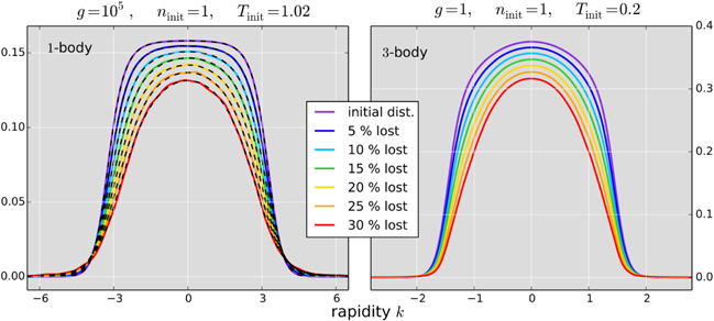
Figure 25. Rapidity distributions of the homogeneous 1D Bose gas, initially at thermal equilibrium at temperature Tinit, after a fraction of the atoms have escaped the system because of K-body loss processes. (Left) Results for one-body losses in the hard-core limit. The colored lines are obtained by evaluating the functional F[ρ](θ) (equation (112)) numerically, with a Monte Carlo summation over eigenstates. The black dashed line is the analytical result available for the hard-core limit. (Right) Numerical results for three-body losses at finite repulsion strength (γ = 1 in the initial state). Reproduced from (Bouchoule et al 2020). CC BY 4.0.
Download figure:
Standard image High-resolution imageUntil very recently not much was known about the evolution of other charge densities. Hutsalyuk and Pozsgay (2020) focused on the energy density and managed to compute the rhs of (118) as an explicit functional of the rapidity distribution ρ(θ). It is likely that their method can be generalized to some other charge densities, and this could perhaps ultimately lead to the variation of the full distribution of rapidities. At the moment, nothing is known beyond the atom density and the energy density though, and finding expressions similar to those of Bastianello et al (2018), Hutsalyuk and Pozsgay (2020), Pozsgay (2011) for the variation of other charges remains an open problem.
Again, we also refer the reader to the review of Bastianello et al (2021) in this volume for a thorough discussion of related recent results.
5.3. 1/θ4 tails in the rapidity distribution
One striking effect of losses is found when investigating the evolution of the high-rapidity tails of the rapidity distribution ρ(θ). It was shown in (Bouchoule and Dubail 2020) that, under losses, ρ(θ) develops algebraically decaying tails, ρ(θ) ∼ 1/θ4 when |θ| → ∞. This is in contrast with more standard cases of rapidity distributions, e.g. those in thermal equilibrium states, which typically decay exponentially or even as Gaussians.
The physical origin of the development of those 1/θ4 tails in the rapidity distribution lies in the cusp singularity of the wavefunction when two atoms are at the same position, see equation (9):

Consider the case of one-body losses (K = 1), for simplicity. At a time tl
, the lth atom is suddenly removed from the system. Immediately after the loss event, the wavefunction of the remaining atoms is  , where xl
is the position of the lost atom. This wavefunction, viewed as a function of xi
, still has a cusp singularity at xi
= xl
, even though there is no longer a particle at xl
. On the other hand, the eigenstates of the Lieb–Liniger Hamiltonian (6) for N − 1 atoms are smooth functions of zi
around zi
= zl
(for fixed values of xj
≠ xl
for j ≠ i). Expanding the wavefunction
, where xl
is the position of the lost atom. This wavefunction, viewed as a function of xi
, still has a cusp singularity at xi
= xl
, even though there is no longer a particle at xl
. On the other hand, the eigenstates of the Lieb–Liniger Hamiltonian (6) for N − 1 atoms are smooth functions of zi
around zi
= zl
(for fixed values of xj
≠ xl
for j ≠ i). Expanding the wavefunction  over the eigenstates for N − 1 particles, one finds that the coefficients of the Bethe states
  decay as
  . The rapidity distribution is obtained by averaging w.r.t. to the squared amplitudes of these coefficients, so it must decay as 1/θ4.
Rapidity distributions decaying as 1/|θ|4 are not very common, however, there is at least one other known physical scenario where they appear: a sudden quench of the repulsion strength g. In (De Nardis et al 2014), the rapidity distribution ρ(θ) after a quench from g = 0 at zero temperature (BEC) to g > 0 is computed exactly, and it is found that ρ(θ) ∼ 1/θ4 for large rapidities. Notice that this is consistent with the discussion above based on cusps of the wavefunction: when the repulsion strength g is suddenly changed, the wavefunction immediately after the quench violates the cusp condition (119), resulting in an expansion over Bethe states with coefficients decaying slowly at large rapidities, as in the case of losses.
One important physical consequence of the presence of the 1/θ4 rapidity tails, worked out in (Bouchoule and Dubail 2020), is the breakdown of a famous exact relation between the tails of the momentum distribution w(p) in the gas and the ‘contact’ (Minguzzi et al 2002, Olshanii and Dunjko 2003),

Here the momentum distribution w(p) is normalized such that ∫w(p)dp = n. The relation (120) has been extended to higher dimensions and to fermionic gases or general Bose–Fermi mixtures with contact interaction (Tan 2008a, 2008b, 2008c). It is known as ‘Tan’s adiabatic theorem’ or simply ‘Tan’s relation’, and it has been studied extensively over the past 15 years, both theoretically—see e.g. (Barth and Zwerger 2011, Braaten and Platter 2008, Minguzzi et al 2002, Olshanii and Dunjko 2003, Tan 2008a, 2008b, 2008c, Werner and Castin 2012a, 2012b, Yao et al 2018)—and experimentally (Kuhnle et al 2010, Stewart et al 2010, Wild et al 2012).
However, in (Bouchoule and Dubail 2020), it is argued that the relation (120) breaks down when the rapidity distribution decays as 1/θ4 at large θ. In that case, the rapidity tail adds to the one caused by the two-body contact term. More precisely, introducing Cr = limθ → ∞ ρ(θ) θ4 the amplitude of the 1/θ4 rapidity tails, the relation (120) is superseded by the relation

In most known stationary states of the gas, in particular in thermal equilibrium states, Cr = 0, so that Tan’s relation (120) holds. However, in a gas subject to losses, or after a quench of the interaction strength g, Cr > 0 and Tan’s relation is violated. Moreover, in (Bouchoule and Dubail 2020), the amplitude of the term Cr is found to be potentially much larger than 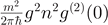 . For one-body losses (K = 1) the ratio
 ![${C}_{\text{r}}/[\frac{{m}^{2}}{2\pi \hslash }{g}^{2}{n}^{2}{g}^{(2)}(0)]$](https://content.cld.iop.org/journals/1742-5468/2022/1/014003/revision6/jstatac3659ieqn171.gif) increases exponentially in time under lossy evolution, while it grows logarithmically for K = 2 and remains bounded (but not necessarily close to one) for K ⩾ 3.
increases exponentially in time under lossy evolution, while it grows logarithmically for K = 2 and remains bounded (but not necessarily close to one) for K ⩾ 3.
5.4. Results in the quasicondensate regime
In the asymptotic regime of a quasicondensate, the effect of losses can be investigated using the Bogoliubov description of the gas. The Bogoliubov approach is an approximate description of the gas, that constitutes a trivial integrable model since it amounts to independent bosonic modes: the integrals of motion are nothing other than the population in each mode. The effect of losses within the Bogoliubov approach was first investigated in (Grišins et al 2016, Rauer et al 2016), where the emphasis was put on the long-wavelength modes, the so-called phononic modes. These studies were then extended to all Bogoliubov modes, and also to K-body processes (Bouchoule et al 2018, Johnson et al 2017). The population of the phononic modes is expected to reach a value corresponding to a temperature Tp that fulfills

where μ ≃ gn is the chemical potential of the gas and α is a numerical factor, of order one, which depends on K. This prediction is in agreement with experimental studies made for three-body (Schemmer and Bouchoule 2018) and one-body (Bouchoule and Schemmer 2020) losses. Bogoliubov modes of shorter wavelength are, on the other hand, expected to reach a higher temperature (Grišins et al 2016, Johnson et al 2017). This peculiar state, in which the temperature of the short-wavelength modes is larger than that of the phonons, might be the reason for the experimental observation of long-lived non-thermal states (Johnson et al 2017).
The integrals of motion of the Bogoliubov model are however not the real integrals of motion, which are given by the rapidity distribution. The precise link between the Bogoliubov modes and the rapidities is still an open question. For short-wavelength modes, however, one can identify the population of the Bogoliubov modes with rapidities, as done already by Lieb (1963) in a seminal contribution. When doing this identification, the results of the Bogoliubov theory for the effect of losses on short-wavelength modes coincide with the expected behavior for the tails of the rapidity distribution (Bouchoule and Dubail 2020). For the phonons, on the other hand, there is no one-to-one correspondence with rapidities. Neither the validity of equation (122) at long terms, nor its compatibility with the time evolution of the rapidity distribution, has been established yet.
5.5. Other related recent results
In (Rossini et al 2020), a lattice Bose gas with onsite repulsion (the Bose–Hubbard model) and onsite two-body losses is studied. In the limit of very fast losses, all configurations with more than one particle per site decay extremely quickly, so the slow dynamics occurs within the restricted subspace of configurations with at most one boson per site. In the effective dynamics of these emerging hard-core lattice bosons, two-body losses are still present, however, they occur on nearest-neighbor sites and they are very slow (García-Ripoll et al 2009). Thus, Rossini et al (2020) effectively work with a lattice hard-core boson model subject to adiabatic two-body losses. The corresponding (lattice) rapidity distribution is evaluated in a way that parallels the above discussion, see equation (112), and results analogous to those of Bouchoule et al (2020) are obtained.
As mentioned above, losses in the Lieb–Liniger gas are but one particular example of a mechanism that breaks the integrability of the underlying model. Other mechanisms have been studied, for instance the coupling between tubes in an array of 1D gases (Caux et al 2019), or dephasing (Bastianello et al 2020b). Let us also mention closely related works on integrable spin chains evolving under Lindblad evolution (Lange et al 2017, 2018, Lenarčič et al 2018), where an adiabatic limit analogous to the one discussed above is implemented using truncated GGEs, or the crossover from ballistic to diffusive transport induced by weak integrability breaking terms (Friedman et al 2020, Žnidarič 2020). These results, and more, are discussed in the review of Bastianello, De Luca and Vasseur in this volume.
6. Conclusion and perspectives
GHD theory has proven to be very efficient at describing non-equilibrium dynamics in 1D Bose gases. Its broad applicability domain has been confirmed by the first experimental tests. Nevertheless, investigation of non-equilibrium dynamics using the GHD theory is still in its infancy. Many situations are still to be explored. On the experimental side, it would be interesting to investigate the so-called bi-partite quench protocols where two clouds with different rapidity distributions and separated by a barrier at x = 0 are merged by a sudden removing of the barrier. This fundamental problem in the theory of gases and in hydrodynamics—where it is usually known as a Riemman problem (Riemann 1860)—seemed completely out of reach in integrable spin chains and integrable gases before 2016, and it played a major role in the discovery of Bertini et al (2016) and Castro-Alvaredo et al (2016). For an experimental study of this setup, a complete characterization of the system, and the implementation of local measurements in such non-equilibrium protocols, would constitute great progress.
At the heart of GHD there is the idea that the gas is locally described by its rapidity distribution. While the meaning of the rapidity distribution and its time evolution under GHD is quite transparent in the hard-core regime, where it simply corresponds to the momentum distribution of the equivalent ideal Fermi gas, it is less obvious in the weakly interacting case. On the other hand, in weakly interacting regimes, powerful techniques have been developed, such as the Bogoliubov techniques or the classical field approach. Making the link between those approximate techniques and GHD, including the notion of rapidity distribution, would be substantial progress. The Bogoliubov model is a trivially integrable model, although its integrals of motion are not the true integrals of motion of the underlying Lieb–Liniger model. Some open questions are: what are the Bogoliubov distributions which are stationary with respect to the Lieb–Liniger dynamics? What is the Bogoliubov distribution of a given rapidity distribution? Vice versa, what is the rapidity distribution of a given Bogoliubov distribution? At sufficiently high temperatures such that quantum fluctuations become negligible, one can describe the gas within the classical field framework. The link between GHD and classical field predictions also deserves more investigation.
Many-body dynamics in 1D Bose gases is a wide research area, and the effects that can be described within the GHD framework are, presumably, only a small part of it. It is of great interest to study phenomena that are beyond the original GHD theory. Many questions have still to be elucidated, and we propose here a non-exhaustive list of research directions.
- Beyond the 1D regime. In experiments, physics lies in the 3D space, and the 1D model is only an approximated description. Effects that are beyond the 1D physics still need investigation. In the case of a harmonic transverse trap, the effect of transversely excited states is not completely established yet. In (Møller et al 2021), a first theoretical framework was proposed to take into account atoms populating a higher transversely excited state. On the experimental side, the thermalization observed by Li et al (2020) in the quantum Newton cradle setup is attributed to the presence of atoms in transversely excited states. In this experiment, relaxation occurs for a gas lying in the ideal Bose gas regime. Exploring other regimes would be highly desirable. Even if the transverse degree of freedom is energetically frozen, transversely excited states may play a role as intermediate states in virtual three-body processes (Mazets et al 2008). Such an effect, which is of course beyond the GHD theory, is expected to lead to thermalization of the gas. How this thermalization occurs is an open question.
Another situation that goes beyond the 1D model is the case of an array of 1D tubes coupled by a small tunnel effect. Again, the effect of such a coupling on the evolution of the rapidity distribution is not known. One expects that this coupling will permit thermalization. This situation allows the study of the dimensional crossover between 1D and 2D or 3D physics.
- Diffusion effect. GHD, which was initially formulated in the Euler limit, has been extended by the addition of a Navier–Stokes diffusive term. The experimental test of such a diffusive term would be an important achievement.
- Breakdown of integrability due to a potential. The combined effect of the diffusive term in GHD and of a spatially varying external potential is expected to lead to a relaxation toward a thermal state, as shown in numerical simulations reproducing the Newton cradle setup. From the theoretical viewpoint, different situations could be considered. On the experimental side, such an effect has not been observed, probably because the potentials are usually varying over distances that are too large. The experimental investigation of such an effect would certainly increase understanding of the phenomenon.
We would like to finish this conclusion with some considerations on the effects of losses. As seen in the recent studies presented above, the effect of losses is highly non-trivial. Even one-body losses, whose effect is trivial for a non-correlated gas, have a non-trivial effect in the presence of interactions between atoms. This is also true in higher dimensions. Higher-dimensional gases, when they are interacting, are not integrable, such that the effect of adiabatic losses can be characterized by the time evolution of only two quantities: the particle density and the energy density. However, the computation of the latter still needs to be done. Thus, amazingly, the effect of losses is now better understood in 1D gases, where it is a priori more complicated since one has to keep track of the whole rapidity distribution, than in higher dimensions.
Acknowledgments
We have greatly benefited from discussions with many colleagues. Among them, we would like to thank especially our co-authors on the topics reviewed in this article: Julien Armijo, Maxim Arzamasov, Yasar Yilmaz Atas, Alvise Bastianello, Pasquale Calabrese, Jean-Sébastien Caux, Benjamin Doyon, Bess Fang, Dimitri Gangardt, Thibaut Jacqmin, Aisling Johnson, Karen Kheruntsyan, Robert Konik, Yuan Le, Neel Malvania, Marcos Rigol, Tommaso Roscilde, Paola Ruggiero, Max Schemmer, Gora Shlyapnikov, Jean-Marie Stéphan, Stuart S Szigeti, David Weiss, Takato Yoshimura and Yicheng Zhang. We are also grateful to David Weiss, Frederik Møller and Jörg Schmiedmayer for comments on the manuscript. This work was supported by the ANR Project QUADY-ANR-20-CE30-0017-01.