ABSTRACT
Direct detection of thermal emission from nearby hot Jupiters has greatly advanced our knowledge of extrasolar planets in recent years. Since hot Jupiter systems can be regarded as analogs of high-contrast binaries, ground-based infrared long-baseline interferometers have the potential to resolve them and detect their thermal emission with precision closure phase—a method that is immune to the systematic errors induced by the Earth’s atmosphere. In this work, we present closure-phase studies toward direct detection of nearby hot Jupiters using the CHARA interferometer array outfitted with the MIRC instrument. We carry out closure-phase simulations and conduct a large number of observations for the best candidate υ And. Our experiments suggest that the method is feasible with highly stable and precise closure phases. However, we also find much larger systematic errors than expected in the observations, most likely caused by dispersion across different wavelengths. We find that using higher spectral resolution modes (e.g., R = 150) can significantly reduce the systematics. By combining all calibrators in an observing run together, we are able to roughly recalibrate the lower spectral resolution data, allowing us to obtain upper limits of the star-planet contrast ratios of υ And b across the H band. The data also allow us to get a refined stellar radius of 1.625 ± 0.011 R⊙. Our best upper limit corresponds to a contrast ratio of 2.1 × 10³ : 1 with 90% confidence level at 1.52 μm, suggesting that we are starting to have the capability of constraining atmospheric models of hot Jupiters with interferometry. With recent and upcoming improvements of CHARA/MIRC, the prospect of detecting emission from hot Jupiters with closure phases is promising.
1. INTRODUCTION
The discovery of a planet around a nearby star 51 Peg in 1995 opened a window into new worlds outside the solar system (Mayor & Queloz 1995). Since then, more than 500 so-called exoplanets7 have been discovered, revolutionizing our knowledge of their nature and origin. Among those discoveries, about 24 planets had their thermal emission directly detected by photometric and/or spectroscopic measurements from space or ground, most of which are known as “hot Jupiters” or “hot Neptunes” (e.g., Deming et al. 2005; Charbonneau et al. 2005; Harrington et al. 2006; Alonso et al. 2009; Sing & López-Morales 2009; Machalek et al. 2010; Stevenson et al. 2010; Croll et al. 2010; etc.). So far, direct detection of thermal emission and characterization of planetary atmospheres is generally only possible for these hot planets, as they are very close to their host stars (< 0.1 AU) and are thus heated enough to have temperatures above 1000 K, providing as high as 10-3 of their host stars’ flux in the infrared (e.g., J, H, K, and mid-infrared).
The atmospheres of hot Jupiters have many interesting properties. For instance, transmission spectra at primary eclipses have shown the presence of sodium, water, and methane (e.g., Redfield et al. 2008; Swain et al. 2009), while thermal emission at secondary eclipses has shown the presence of water, carbon dioxide, and carbon monoxide (e.g., Knutson 2007a; Barman 2008; Swain et al. 2008). Due to their close-in orbits, hot Jupiters are tidally locked to their host stars, leading to a constant day side that experiences intense stellar irradiation and a cold night side that remains in perpetual shadow (Guillot et al. 1996). The temperature difference between the day and night sides thus induces atmospheric circulation and strong zonal winds to redistribute the heat (Knutson 2007b). Studies have also suggested the existence of a hot stratosphere on the day side of some hot Jupiters (e.g., HD 209458b and HD 149026b), which inverts the temperature profile of higher atmospheric layers and flips water absorptions into emissions (Knutson et al. 2008; Burrows et al. 2008; Madhusudhan & Seager 2010). However, some other planets such as HD 189733b seem to lack such thermal inversion (Charbonneau et al. 2008; Grillmair et al. 2008), implying fundamental atmospheric differences between these planets and leading to subclassification of hot Jupiters (Burrows et al. 2008). Studies of hot Jupiters’ atmospheres will not only reveal their composition, structure, and dynamics, but will also shed light on our understanding of the planet formation processes. More importantly, characterizing hot Jupiters allows us to pave the path toward characterizations of Super-Earth planets and, eventually, Earth-like planets.
Among the ∼22 detected hot Jupiters, however, a majority of them are transiting planets whose orbits are aligned with the line of sight from the Earth, and only two of them are nontransiting planets (i.e., υ And b and HD 179949b; Harrington et al. 2006; Cowan et al. 2007). The lack of studies of nontransiting hot Jupiters leaves a great opportunity for long-baseline optical/infrared interferometry, in that long-baseline interferometers can see hot Jupiter systems as extremely high-contrast binaries and thus can directly determine their orbital elements and provide accurate mass estimates. Interferometric measurements can also provide absolute planet/star flux ratios (or star/planet contrasts) of nontransiting planets that cannot be disentangled by combined-light techniques (i.e., through transits). In fact, interferometric measurements also provide an independent way of characterizing transiting planets in addition to the combined-light technique. Since the bulk of energy from hot Jupiters emerges from the near-IR between 1–3 μm (Burrows et al. 2008), interferometry can provide a better understanding of their spectra and global energy budget with measurements at near-IR bands.
However, detecting the weak emission from a hot Jupiter from the ground is a difficult task. To date, only a few hot Jupiters’ thermal emissions have been detected from the ground, while the rest were all achieved from space. To reach this goal, we require very stable and high-precision measurements and, most importantly, require a method that can eliminate or calibrate the effects of Earth’s atmospheric turbulence. One possible approach is to use high-precision and high-resolution closure-phase measurements obtained with ground-based interferometers. Closure phase is measured by combining the phases of three baselines in a closed triangle. It is immune to any phase shifts induced by the atmospheric turbulence, including the differential chromatic dispersion that affects the differential phase. The major biases or systematic errors of closure phase come from nonclosed triangles introduced in the measurement process and, in principle, can be precisely calibrated. Therefore, it is a good observable for stable and precise measurements. More descriptions of the closure-phase technique can be found in Monnier (2003, 2007).
Studies have already been carried out to explore the possibilities of using closure phases for exoplanet detection (e.g., Joergens & Quirrenbach 2004; Zhao et al. 2008a, etc.). Particularly, Chelli et al. (2009) studied in detail the characteristics of closure phases and the corresponding signal-to-noise ratio (S/N) when the primary star of a binary is getting resolved and approaching the visibility null (i.e., phase closure nulling). Using this method, Duvert et al. (2010) detected the faint close companion of HD 59717 at a contrast of ∼100∶1 using VLTI/AMBER. Recently, Absil et al. (2010) also excluded the presence of a brown-dwarf companion in the innermost region of the β Pic planetary system at a upper contrast limit of ∼200∶1 using closure phases obtained by VLTI/AMBER.
In this article, we report our closure-phase studies toward the ultimate goal of directly detecting emission from hot Jupiters using the Center for High Angular Resolution Astronomy (CHARA)/MIRC. The paper is organized as follows. We first briefly introduce our candidate υ And b and our observations in § 2. In § 3 we simulate the closure-phase signals and the required precision for the candidate. We then discuss the calibration issues we encountered in test observations and present our solutions. Based on our calibrations, we present a preliminary upper limit for υ And b in § 4. Finally, we conclude our studies and give future prospects in § 5.
2. CANDIDATES AND OBSERVATIONS
2.1. Candidates
Among all the known nontransiting hot Jupiters, several of them are within the sensitivity limit of CHARA/MIRC. Currently, υ And b is the most favorable candidate due to its relatively high temperature and the high brightness of its host star. Therefore, in this study we focus only on this best candidate.
The F8V star υ And is located 13.5 pc away from the Sun. Butler et al. (1997) first discovered its hot Jupiter υ And b in 1997, which has a period of 4.6 days and is orbiting at 0.06 AU. The follow-up observations of Butler et al. (1999) found two more companions in the system, υ And c and υ And d. The second planet υ And c is orbiting at 0.83 AU from the host star with a period of 241 days, while υ And d is orbiting at 2.5 AU with a period of 1267 days (Butler et al. 1999). Most recently, Curiel et al. (2011) found a fourth planet υ And e with a period of 3848.9 days at 5.25 AU. The system is noncoplanar. The inclination of the closest planet υ And b is found to be likely ≥28° (Crossfield et al. 2010), while the second and the third planets (υ And c and υ And d) have a relative inclination of 15°–20°. In 2006, Harrington et al. (2006) directly detected thermal emission from the hot Jupiter υ And b using the Spitzer multiband imaging photometer (MIPS) at 24 μm, in which they detected the relative day-night flux variations of the planet over five epochs of the whole 4.6 day orbital period and provided a lower limit to the planet/star flux ratio. Later, Crossfield et al. (2010) further refined the flux variation curve with more MIPS 24 μm data and found an unusually large phase shift of the flux maximum (∼80°). Atmospheric models have also been applied to interpret these Spitzer data. However, as Burrows et al. (2008) pointed out, due to the lack of absolute flux level and information in other wavelengths, there are too many degrees of freedom to draw strong conclusions about the planetary and atmospheric properties. Thus, detection of its absolute planet/star flux ratios and at other wavelengths such as near-IR is required to break model degeneracies. Furthermore, high-S/N detections will even allow us to obtain the absolute phase curve of the planet (Barman et al. 2005), providing constraints to the circulation and heat redistribution patterns of its atmosphere.
2.2. Observations
Closure-phase measurements require at least three telescopes to be combined in a closed triangle. Currently, the Michigan Infra-Red Combiner (MIRC; Monnier et al. 2004) and Classic Infrared Multi-Beam combiner (CLIMB; Sturmann et al. 2010) instruments at the CHARA array and the Astronomical Multi-Beam combiner (AMBER; Petrov et al. 2007) and Precision Integrated Optics Near-infrared Imaging Experiment (PIONIER)8 instruments at the Very Large Telescope Interferometer (VLTI) have this capability in the near-IR. In this study, we employ CHARA/MIRC for our measurements.
The CHARA array, located on Mount Wilson, consists of six 1 m telescopes (ten Brummelaar et al. 2005). The array is arranged in a Y-shaped configuration to provide good position angle coverage. The six telescopes form 15 baselines ranging from 34 m to 331 m, making CHARA the longest-baseline optical/IR interferometer array in the world and providing a resolution of ∼0.5 mas in the H band. MIRC is an imaging combiner that currently combines four CHARA telescopes, providing six visibilities, four closure phases, and four triple amplitudes simultaneously. MIRC works at both H and K bands, and has three spectral modes: R = 40 (with prism), 150, and 500 (with grism). The lowest-resolution mode (R = 40) disperses light into eight spectral channels on the detector, while the R = 150 and R = 500 modes disperse light into 24 channels and 80 channels, respectively (see Monnier et al. 2004, 2006 for details). The compact design of MIRC allows for stable calibration and precise closure-phase measurements; thus,x it is best suited for the purpose of this study.
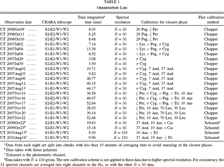
We conducted observations of υ And on 23 nights from 2006 to 2010 with a total integration time of 8.2 hr, following the standard observing procedures (Monnier et al. 2007; Zhao et al. 2009). The observation log is listed in Table 1. Several combinations of four CHARA telescopes are used in the observations, while in most cases we adopt the combination S1-E1-W1-W2 and S2-E2-W1-W2 for good baseline coverage. The observations were mostly conducted in the H band (λ = 1.5–1.8 μm) with the lowest-resolution mode of R = 40, except for two nights in 2010 when we employed the higher-resolution mode of R = 150. Each observation of the target was bracketed with calibrators for visibility and closure-phase calibration. For the purposes of bias subtraction and flux calibration, each set of fringe data is bracketed with measurements of background (i.e., data taken with all beams closed), shutter sequences (i.e., data taken with only one beam open at a time to estimate the amount of light coming from each beam), and foreground (i.e., data taken with all beams open, but without fringes) (Pedretti et al. 2009). Each object is observed for multiple sets. During the period of taking fringe data, a group-delay fringe tracker is used to track the fringes (Thureau et al. 2006). In order to track the flux coupled into each beam in real time to improve the visibility measurements, we used spinning choppers to temporally modulate the light going into each fiber simultaneously with fringe measurements. In 2009, photometric channels were commissioned for MIRC (Che et al. 2010), and the choppers were made obsolete because of the much better real-time flux calibration provided by the photometric channels. The data reduction process also follows the pipeline outlined in Monnier et al. (2007), where the closure phases are extracted from the phase term of the complex triple amplitudes after the subtraction of background, foreground, and correction of fiber coupling efficiencies.
 |
3. CLOSURE-PHASE SIMULATIONS AND CALIBRATION STUDIES
3.1. Simulations
Because exoplanet-host stars and their hot Jupiters are similar to high-contrast close binaries, we simulate the closure-phase signals using binary models for υ And b. We choose to use the longest telescope triangle of the CHARA array (i.e., S1-E1-W1) in our study to obtain the highest closure-phase levels (Chelli et al. 2009). The latest orbital properties of υ And b and the size of its host star are listed in Table 2. The infrared planet/star flux ratios are adopted from the models of Sudarsky et al. (2003).
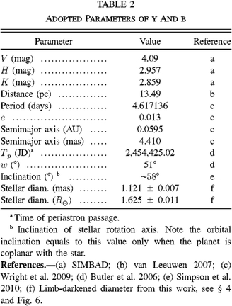 |
Figure 1 shows the closure-phase simulations for υ And b at four wavelength channels. Since the value of the ascending node (Ω) is unknown for υ And b, we assume four different values in our simulations: Ω = 0°, 45°, 90°, and 135°. The inclination is fixed to the most probable values, assuming that the planet is coplanar with the star’s rotation (see Table 2). Figure 1 shows that the closure-phase signal varies rapidly as the baseline projection varies during the Earth’s rotation. Shorter-wavelength channels generally have higher signal amplitudes and peak at ∼ ± 0.08°, due to the fact that the host star is more resolved at those wavelengths. The overall closure-phase level of υ And b is insensitive to the values of Ω in the simulation because of CHARA’s even baseline layout (i.e., the Y shape), which covers all position angles more or less equally well. We note here that because the visibility of the star υ And only goes to null at certain wavelength channels, the closure-phase signal in the simulation is very sensitive to the value of adopted stellar diameter. Figure 1 also indicates that in order to detect the closure-phase signal from υ And b, the required 1-σ precision has to be better than roughly ± 0.05°.
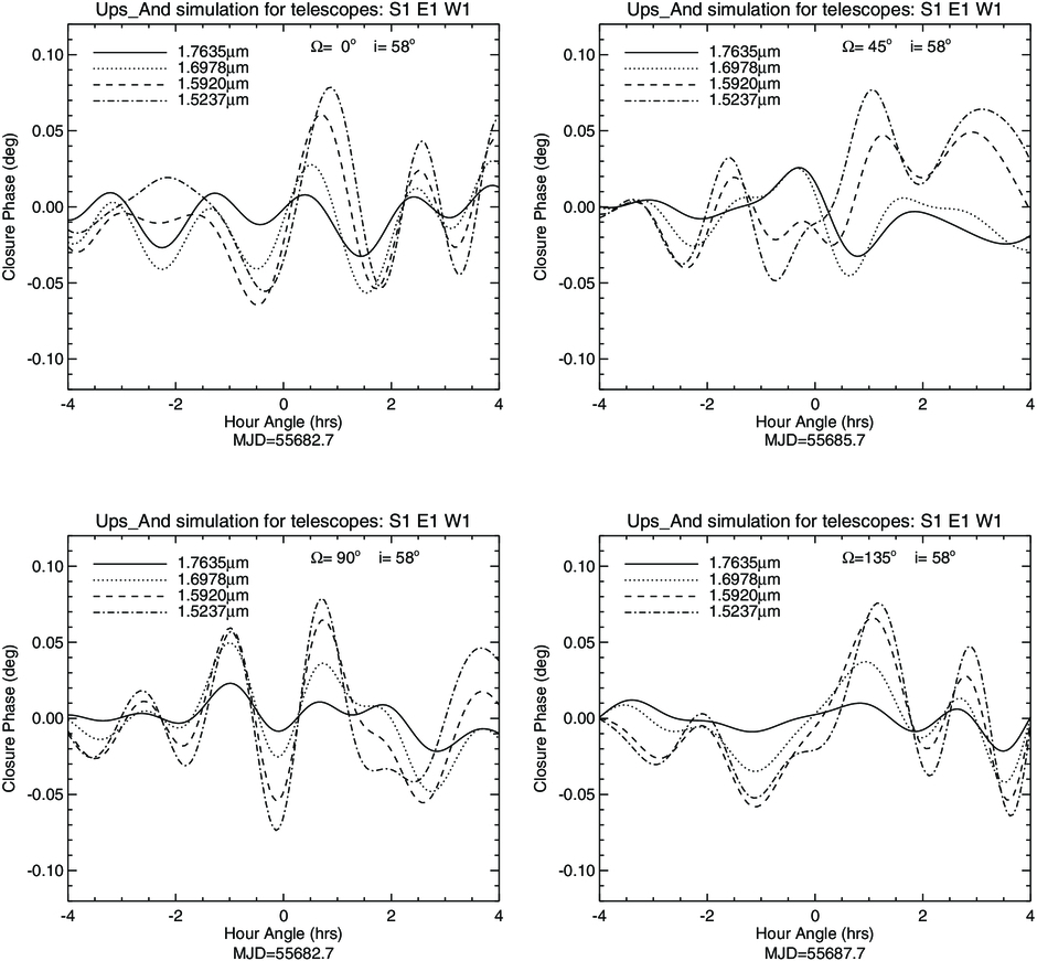
Fig. 1.— Closure-phase simulation of υ And b, using the largest triangle of CHARA, S1-E1-W1, and corresponding to an angular resolution of 0.5 mas in the H band. Four out of eight wavelength channels of MIRC in the H band are shown. The planet/star flux ratios of the four channels (1.52 μm, 1.59 μm, 1.70 μm, and 1.76 μm) are 0.27 × 10⁻⁴, 0.47 × 10⁻⁴, 0.6 × 10⁻⁴, and 0.35 × 10⁻⁴, respectively (Sudarsky et al. 2003). The orbital parameters used in the simulation are listed in Table 2. The four panels assume Ω = 0°, 45°, 90°, and 135°, respectively. The dates of the simulation are chosen arbitrarily. Due to the even baseline layout of CHARA, the signal level of the closure phase is insensitive to the values of Ω, although the maximum signal may occur at different times.
3.2. Calibration Studies
To compare the precision of our measurements with the simulations, we first examine the quality and stability of our data. The left panels of Figure 2 show a good night of closure-phase measurements for the middle wavelength channel of MIRC, obtained with the largest triangle of CHARA (S1-E1-W1). The closure phases are stable over the 1.5 hr of observation, and the error averages down roughly as  (the bottom left panel), suggesting that the measurements are immune from systematic errors like changes in the seeing. The nominal measurement error is 0.3° when averaging the whole 1.5 hr of observation together. The performance at a similar channel with a shorter triangle of CHARA (E2-W1-W2) is demonstrated to be about 3 times better in Zhao et al. (2008b).
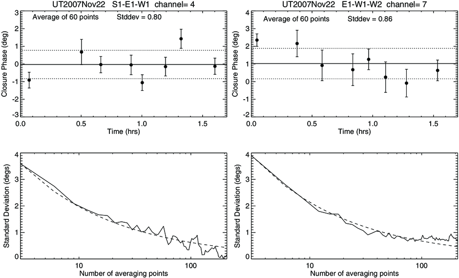
Fig. 2.— Test observation of υ And using the outer array (S1-E1-W1-W2) of CHARA from 2007 November 22. The top panels show the 60-point averaged data, corresponding to 320 s of integration time. The solid lines in the top panels indicate the average closure-phase levels, while the dashed lines indicate 1-σ deviation from the average. The bottom panels compare the averaged closure phases with the standard  law for normally distributed errors, i.e., without systematics. The bottom right panel shows that the errors of that channel cannot be averaged down beyond 60 averaging points, due to the systematic drift.
Although these measurements are promising and stable, we have also encountered large unexpected systematic errors in other wavelength channels. As indicated in the right panels of Figure 2, the closure phases show a systematic drift and the associated errors cannot be averaged down as  . In fact, the closure phases not only change with time, but also vary as a function of wavelength. More interestingly, the closure-phase drifts are highly correlated for all calibrators within a whole observing run of many nights. Figure 3 plots closure phases of six calibrators obtained in six nights in 2008 August (Algenib, 38 Tau, γ Lyr, γ Tri, ζ Peg, and ζ Per) versus azimuth angles. There is a clear trend of closure-phase change as a function of azimuth in the figure. Figure 4 shows the similar correlation of closure phase with altitude. The closure-phase drift reaches about 8° between the top and the bottom panels. In addition, we can also see an obvious slope change centered at the middle wavelength channels in both Figures 3 and 4. Although only three wavelength channels are shown here, the slope actually changes gradually from the first to the last channels of MIRC, and similar effects are also seen in other observing runs. Although the data shown in these figures were obtained in six nights, the correlations with altitude and azimuth are strong and consistent, suggesting that the major cause of the closure-phase drifts may stem from the changing positions of the targets on the sky.
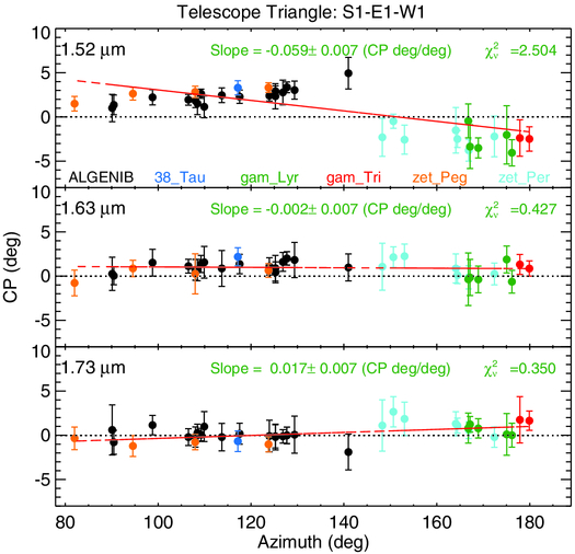
Fig. 3.— Closure phase vs. azimuth for six calibrators in 2008 August. The first, middle, and last wavelength channels of MIRC are shown from top to bottom. The data were taken with telescope S1-E1-W1. The red line shows the linear fit of closure phase as a function of azimuth. Different colors indicate different targets. The slope of the linear fit and the reduced χ2 are also labeled in each panel.
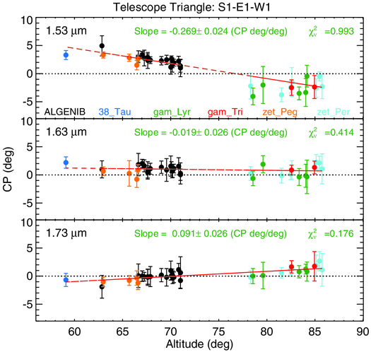
Fig. 4.— Closure phase vs. altitude for six calibrators in 2008 August. The red line shows the linear fit of closure phase as a function of altitude. Different colors indicate different targets. The parameters of the fits are also shown in each panel. The best fits are good and within the scatter and error bars of the data.
Possible causes of the closure-phase drifts may include 1) polarization effects caused by the nonidentical beam trains of CHARA and 2) extra dispersions in the delay lines that are not compensated in vacuum, which can contaminate closure phases across wavelength channels and change with target position. To investigate the individual causes and find the best solution, we carried out a series of experiments with 1) using a linear polarizer to reduce the effect of polarization, 2) using a linear polarizer and a 40 μm slit to reduce the effect of polarization and partially reduce dispersion, and 3) using a grism of R ∼ 150 to reduce dispersion only. We determine the slopes of the closure-phase change as a function of only altitude, for simplicity. Since the slopes of the closure phases also drift across wavelength channels (see Fig. 4), we use the magnitude of the slope change (i.e., slope of channel 8 minus slope of channel 1) to characterize the closure-phase changes. The magnitudes of slope change are averaged over four closure-phase triangles of each observing run, and the errors are determined from the scatter of the four triangles. The results of the experiments are shown and compared in Table 3.
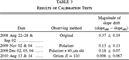 |
Table 3 shows that the original observations have the largest magnitude of closure-phase change. Observations with polarizer and polarizer +40 μm slit have slightly smaller magnitudes of closure-phase change. However, we have also seen some nights without polarizers that have similar or even lower drifts than those with the polarizer, indicating that the effect of using a polarizer is small and the major cause of the drifts may not be polarization effects. When using the grism of R = 150, however, the correlated closure-phase drifts and slope change become nearly zero. Although we only had a very small amount of data for the experiments, this preliminary result indicates that the extra air dispersion from the delay lines is most likely the major cause of the closure-phase drifts, which contaminates closure phases with nonclosed triangles from other wavelengths, especially at the edges of the bandpass. The dispersion effect also explains the slope change centered at the middle wavelength channels seen in Figures 3 and 4.
Since the closure-phase changes shown in Figures 3 and 4 are highly correlated for all nights within an observing run with consistent system and optical settings. We can use all calibrators from a run to look for a solution to calibrate the drifts. We have experimented with several function forms to characterize the slopes, including linear function, linear surface, quadratic surface, etc. A linear surface fit can estimate the closure-phase drifts well, while a quadratic surface fit works the best. Figure 5 shows an example of our best approach of fitting the closure phases with quadratic surface functions of both target altitude and azimuth. The quadratic surface function characterizes the drifts very well for nearly all wavelength channels, as indicated by the improved χ2 values in the plot. Therefore, it can be employed as a new empirical model to calibrate our data within the same observing run.
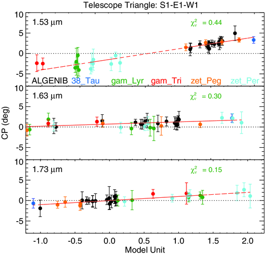
Fig. 5.— Closure phase as a function of azimuth and altitude using quadratic fit. The arrangement and notations are similar to those of Figs. 3 and 4, except that the red line is a fit to the quadratic plane function: a0 + a1·Az + a2·Az2 + a3·Az·alt + a4·Alt + a5·alt2. The reduced χ2 shown in each panel indicate significant improvement than those of Figs. 3 and 4.
There is also a caveat, however, that this calibration scheme requires a wide span of calibrator positions on the sky for a good coverage of altitude and azimuth to bracket the target, so that the quadratic fit can reliably estimate the closure-phase change. However, most of our observations have a limited number of calibrators and calibrator visits and thus do not have a wide range of position coverage. Therefore, we adopt the results from a linear surface fit for those cases instead, in order to avoid unreliable or erroneous quadratic extrapolation, with a tradeoff of slightly less accurate closure-phase calibration. Further validations of these schemes and their robustness are required in a future work.
4. DIAMETER AND UPPER LIMITS FOR υ AND b
4.1. Refined Diameter
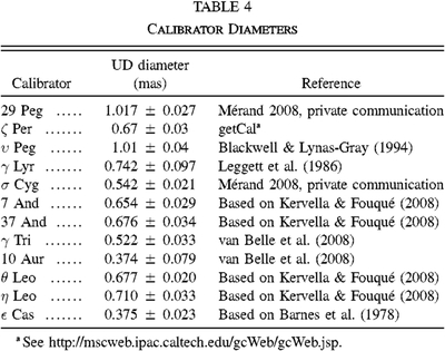
We first determine the angular diameter of υ And with a uniform disk (UD) model and a limb-darkened disk (LD) model. The squared visibilities (V2) of the data are calibrated in the regular way, as described in Monnier et al. (2007). UD diameters of the calibrators are listed in Table 4. We apply a power-law limb darkening, I(μ) = μα, for the LD model (Hestroffer 1997). Since the limb-darkening coefficient α is similar for stars with the same spectral type, we adopt a fixed α and only vary the diameter in our LD fit. The value of α is interpolated and converted from the square root law coefficients of van Hamme (1993). A value of α ≃ 0.18 is estimated for υ And, assuming [Fe/H] = 0.15 (Butler et al. 2006). We bootstrap9 the V2 data from different nights to simulate the statistics. Each bootstrapped data set is then fit with a UD model and a LD model separately with χ2 minimization. A number of 150 bootstrap iterations are carried out, and the median of the 150 best-fit diameters is taken as the global best fit, while the 1-σ error is determined from the scatter. Figure 6 shows the best-fit models of υ And, together with the binned data. Our final best-fit UD of υ And is 1.097 ± 0.009 mas, consistent with the Fiber Linked Unit for Optical Recombination (FLUOR; Coudé du Foresto et al. 2003) measurement of 1.098 ± 0.007 mas (Mérand 2008, private communication) and the results of Baines et al. (2008), 1.091 ± 0.009 mas. The best-fit LD size is 1.121 ± 0.007 mas, also consistent with the result of Baines et al. (2008) and corresponding to a radius of 1.625 ± 0.011 R⊙ for the parallax of 74.12 ± 0.19 mas (van Leeuwen 2007) (with error propagated).
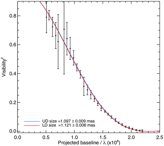
Fig. 6.— Best-fit V2 of υ And with a UD model and a LD model. The V2 data are binned into 30 points for better visualization and are shown as filled dots with error bars. The blue curve shows the best-fit UD model with a reduced-χ2 of 0.37, obtained from the bootstrap process. The best-fit UD diameter from bootstrap is 1.097 ± 0.009 mas. The red line slightly below is the LD model with a reduced-χ2 of 0.36. A power-law limb darkening (Hestroffer 1997) is assumed for the model. The best-fit LD diameter from bootstrap is 1.121 ± 0.007 mas, corresponding to a radius of 1.625 ± 0.011 R⊙ at 13.49 pc.
 |
4.2. Upper Limits
Since we do not have enough S/N to detect the planet from a single night of observation, we can take advantage of the well-known orbital parameters of υ And b and combine all observations in Table 1 to increase the total S/N for higher precision. Due to the quickly varying closure phases caused by the Earth’s rotation, as shown in Figure 1, we split the data into small chunks with an averaging time of less than 10 minutes to avoid smearing the signal.
To calibrate the large closure-phase systematics described in the last section, we apply the new calibration scheme by fitting a quadratic surface function to all calibrators within each observing run and subtracting the predicted zero closure phases from the raw values. For observing runs with inadequate calibrator coverages, we use the results from the linear surface fit instead of the quadratic fit. The total uncertainty of each data point is estimated by bootstrapping the data used in the quadratic or linear surface fit and combining the additional uncertainty with the original values. Figure 7 compares the results before and after applying the new calibration scheme for the 23 nights of data. As we can see in Figure 7, the nonzero closure phases are calibrated out and the large scatters are reduced in the newly calibrated data.
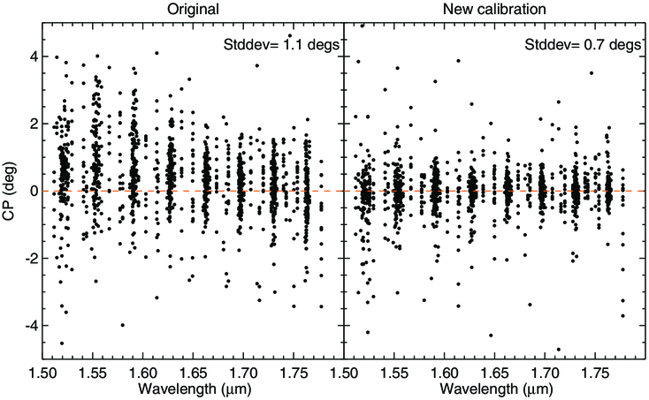
Fig. 7.— Closure phases of υ And before (left) and after (right) the new calibration scheme. Data from all observing nights are overplotted as a function of closure phase vs. wavelength. Due to the variation of wavelength calibration from night to night, the data are scattered around each of the eight wavelength channels of MIRC. The dashed lines represent the reference level for zero closure phases. The scatters of the data are shown in the top right corners.
We then fit the new closure-phase data with binary models to search for the closure-phase signal from the planet. Because the closure phases are different for each channel, we determine planet/star flux ratios for each of the eight wavelength channels simultaneously at the same orbital position and search for the best position with a joint χ2 minimization. The orbital positions of the system are calculated by fixing the well-known parameters from radial velocity observations, i.e., P, T0, e, and ω, and only varying the semimajor axis, Ω, and inclination. The method and the corresponding codes are validated with data of the well-known binary 24 Peg (ι Peg) from Monnier (2007).
Although we have searched the parameter space extensively, we do not clearly detect υ And b in our fits, suggesting that our current signal-to-noise ratio is still inadequate. We thus decided to report our results in terms of an upper limit to the planet/star flux ratio. To do this, we simulate the statistics of the best-fit planet/star flux ratios by bootstrapping different nights of data. This approach treats each night of data equally, ensuring the robustness of the bootstrap by preventing data of certain nights from dominating the statistics. Because noise is dominant in the data, we use a fine grid search to ensure robust results. For each bootstrapped data set, we searched an extensive range of semimajor axis, Ω, inclination, and the planet/star flux ratios at each of the eight spectral channels. The set of parameters that yields the minimum χ2 is then chosen as the best fit. A total of 150 bootstrap iterations are carried out, and the corresponding distributions of the best-fit planet/star flux ratios are shown in Figure 8.
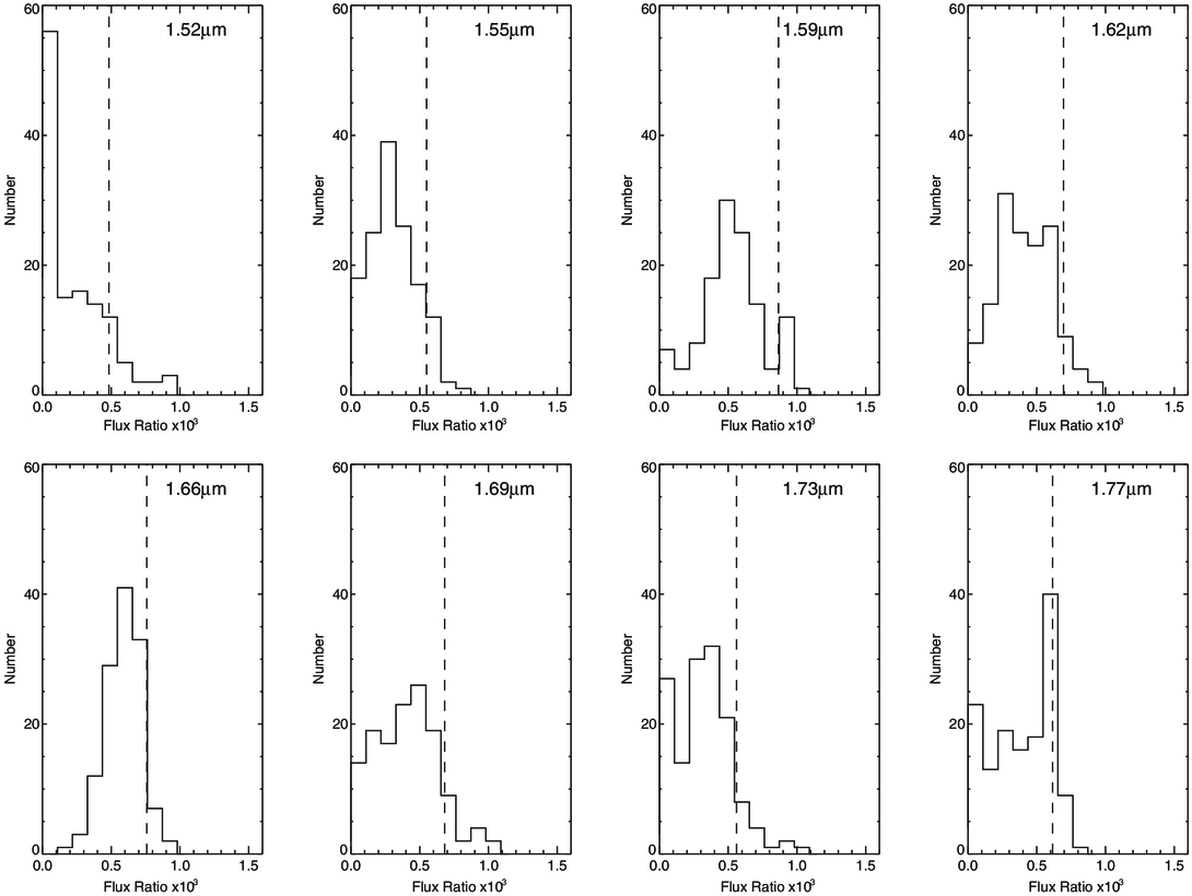
Fig. 8.— Simulated distribution of the best-fit planet/star flux ratios of υ And b in the H band, generated from ∼150 bootstraps of different nights of data. The dashed lines indicate the 90% confidence levels for the upper limits.
The dashed lines in Figure 8 indicate the upper limits of 90% confidence level, i.e., with a 90% chance that these upper limits are higher than the actual planet/star flux ratios. Figure 9 shows the upper limits together as a “spectrum” and compares it with planet atmospheric models based on Barman et al. (2005), Barman (2011, private communication), and Sudarsky et al. (2003). Our upper limits are at the 6 × 10⁻⁴ level, on average. The first channel gives the best limit and reaches a level of 4.7 × 10⁻⁴, corresponding to a star/planet contrast ratio of 2.1 × 10³∶1. This result stands as one of the highest contrast limits achieved by closure-phase measurements to date.
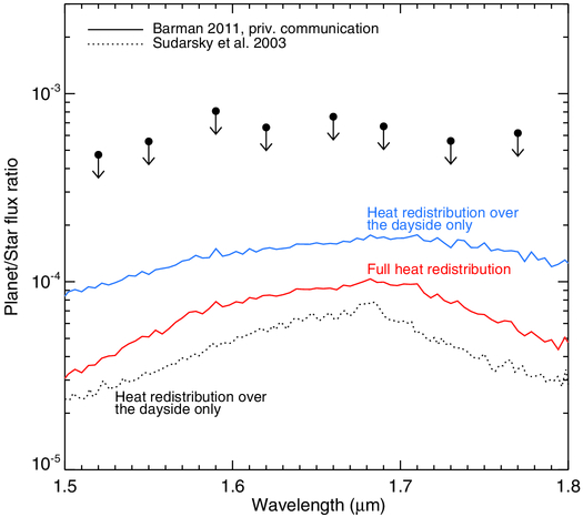
Fig. 9.— Upper limits with 90% confidence levels for the planet/star flux ratios of υ And b in the H band, using the newly calibrated CHARA/MIRC data from multiple nights. The average upper limit level is 6 × 10⁻⁴. The best channel at 1.52 μm shows an upper limit flux ratio of 4.7 × 10⁻⁴. The solid lines show the latest model based on Barman et al. (2005) and Barman (2011, private communication), assuming a typical radius of 1.3 Rj for the planet. The blue line shows the model with incident flux uniformly distributed over the day side of the planet only, while the red line shows the model with full heat redistribution over the entire sphere. The dotted line shows the model prediction from Sudarsky et al. (2003), assuming a radius of 1 Rj with heat redistribution over the day side only.
Our 90% upper limits for the middle channels are about a factor of 5–8 from the predicted value of υ And b, suggesting that with further improvement in precision, we will be able to start constraining atmospheric models for hot Jupiters with interferometry. In fact, the precision of the new calibration for these data is not perfect, due to their lack of wide calibrator coverages on the sky. In addition, although the new calibration can correct for the closure-phase drifts caused by dispersion, the use of calibrators from multiple nights makes the night-to-night variation hard to calibrate, leaving uncorrected systematic errors in the data. To reduce these effects and further improve our calibration precision, the new observing scheme using higher spectral resolution (using the grism of R = 150 for MIRC in this case) and more calibrators is necessary. Benefitting from this experiment and analysis, better precision is expected in future observations.
5. CONCLUSIONS AND FUTURE PROSPECTS
We have simulated the closure phases for the best hot Jupiter candidate υ And b and investigated the precision and stability of our measurements obtained with CHARA/MIRC. Although our closure-phase precisions can reach 0.3° 1.5 hr-1 for the middle wavelength channel of MIRC with good conditions, we have also encountered unexpected closure-phase drifts as large as 8° in other channels. The closure-phase drifts are highly correlated with altitude and azimuth angles of the targets. The slopes of the drifts also vary across spectral channels, centering at the middle channels of MIRC. Because the drifts are correlated for all calibrators within an observing run, we are able to model the trend to calibrate the drifts. This new calibration model, however, is highly dependent on the altitude and azimuth coverage of the calibrators and may not be accurate for sparse coverage. With a set of diagnostics, we find that the closure-phase drifts are most likely caused by extra dispersion in the delay lines, which contaminates closure phases with nonclosed triangles from other wavelengths, especially at the edges of the bandpass. Using higher spectral resolution can effectively reduce this effect. We therefore advocate future observations of CHARA/MIRC to use the grism mode of R = 150 for better calibration precision.
Taking advantage of the well-known orbital parameters of υ And b, we have combined multiple nights of observations for a joint solution of upper limits for the planet/star flux ratios across the H band. Our best upper limit indicates a contrast ratio of about 2.1 × 10³∶1 at 90% confidence level, standing as one of the highest upper limits yet achieved by closure-phase measurements. Future observations with reduced dispersion contaminations using the grism mode are expected to have better performance.
Recently, photometric channels for real-time flux calibration have been implemented for MIRC (Che et al. 2010). The photometric channels have not only improved the visibility calibration, but also improved the data-taking efficiency for MIRC by a factor of ∼2 by reducing the time spent on repositioning fibers of each MIRC beam. The CHAMP fringe tracker for MIRC (Berger et al. 2008) has been commissioned in 2009 and is expected to be fully functional soon. CHAMP will help track and stabilize the fringes to increase their coherence time, allowing longer integration for MIRC, and therefore can increase the S/N to the photon-limited regime and significantly improve the precision. In addition, CHARA is seeking an adaptive optics upgrade (Ridgway et al. 2008) that could increase the throughput of MIRC by at least a factor of 2, which could greatly improve the sensitivity and data-taking efficiency. With these implemented and upcoming improvements and the new observing scheme, we are expecting much better closure-phase performance and are optimistic of achieving the goal of detecting emission from hot Jupiters in the near future.
The CHARA Array is funded by the Georgia State University, by the National Science Foundation through grant AST-0908253, by the W. M. Keck Foundation, and by the NASA Exoplanet Science Institute. Part of this research was carried out at the Jet Propulsion Laboratory, California Institute of Technology, under a contract with the National Aeronautics and Space Administration. This research was supported by the former Michelson Graduate Student Fellowship at the University of Michigan and the NASA Postdoctoral Program at the Jet Propulsion Laboratory (M. Z.). J. D. M acknowledges the NSF grants AST-0352723 and AST-0807577 and the NASA grant NNG04GI33G. E. P. was formally supported by the Michelson Postdoctoral Fellowship and is currently supported by a Scottish Universities Physics Association (SUPA) advanced fellowship. S. T. R. acknowledges partial support from NASA grant NNH09AK731. This research has made use of the SIMBAD database, operated at CDS, Strasbourg, France; the Exoplanets Encyclopedia, maintained by Jean Schneider at Paris Observatory; and the Exoplanet Orbit Database at exoplanets.org.
Footnotes
- 7
Data from The Extrasolar Planets Encyclopaedia: http://exoplanet.eu/catalog.php.
- 8
See http://www-laog.obs.ujf-grenoble.fr/twiki/bin/view/Ipag/Projets/Pionier/WebHome.
- 9
Bootstrapping is a technique that can provide robust simulations of the distribution of a data set. It is very useful for data sets with complicated or unknown distributions and is widely used to derive estimates of standard errors and confidence intervals (Press et al. 1992; Efron & Tibshirani 1993). Since we use multiple nights of data with various baselines and different systematics (within each night) for joint solutions, the distributions of our parameters of interest are unknown. Thus, bootstrapping is a suitable technique for our data. Bootstrapping requires the assumption that the data are independent and identically distributed. This assumption holds for our data, because we treat each night of data equally: each night’s are independent and are acquired in the same way.