ABSTRACT
We investigate the Fermi Large Area Telescope γ-ray and 15 GHz Very Long Baseline Array radio properties of a joint γ-ray and radio-selected sample of active galactic nuclei (AGNs) obtained during the first 11 months of the Fermi mission (2008 August 4–2009 July 5). Our sample contains the brightest 173 AGNs in these bands above declination −30° during this period, and thus probes the full range of γ-ray loudness (γ-ray to radio band luminosity ratio) in the bright blazar population. The latter quantity spans at least 4 orders of magnitude, reflecting a wide range of spectral energy distribution (SED) parameters in the bright blazar population. The BL Lac objects, however, display a linear correlation of increasing γ-ray loudness with synchrotron SED peak frequency, suggesting a universal SED shape for objects of this class. The synchrotron self-Compton model is favored for the γ-ray emission in these BL Lac objects over external seed photon models, since the latter predict a dependence of Compton dominance on Doppler factor that would destroy any observed synchrotron SED-peak–γ-ray-loudness correlation. The high-synchrotron peaked (HSP) BL Lac objects are distinguished by lower than average radio core brightness temperatures, and none display large radio modulation indices or high linear core polarization levels. No equivalent trends are seen for the flat-spectrum radio quasars (FSRQs) in our sample. Given the association of such properties with relativistic beaming, we suggest that the HSP BL Lac objects have generally lower Doppler factors than the lower-synchrotron peaked BL Lac objects or FSRQs in our sample.
1. INTRODUCTION
The successful launch of the Fermi Gamma-Ray Space Telescope in 2008 has brought about a new era in our understanding of blazars, which dominate the extragalactic sky at high energies. Because of their highly variable fluxes and spectral energy distributions (SEDs), blazar samples are typically subject to large biases, making it difficult to study their demographics. With the nearly continuous all-sky monitoring capabilities of Fermi's Large Area Telescope (LAT), however, it is now possible to construct well-defined samples that can be used to investigate the wide range of jet properties in these powerful active galactic nuclei (AGNs; e.g., Abdo et al. 2010d; Kovalev 2009).
One of these properties that has been of considerable interest since the era of the Compton Gamma Ray Observatory (CGRO) in the 1990s is γ-ray loudness, or in other words, why only a particular small subset of known AGNs (∼100; Hartman et al. 1999) were detected by the CGRO's EGRET telescope. Considerable evidence has been presented by many researchers (e.g., Dondi & Ghisellini 1995; Kellermann et al. 2004; Kovalev et al. 2005; Jorstad et al. 2001; Taylor et al. 2007) supporting the idea that relativistic Doppler boosting has a large impact on AGN γ-ray emission, but lingering questions regarding the roles of the flaring duty cycle and the AGN SED remain. The superior sensitivity and full-time survey operation mode of Fermi have now provided substantial insight into these issues. With the release of the 1FGL catalog (Abdo et al. 2010a), the strong impact of SED characteristics on the fainter γ-ray AGN population was realized, as the sky at these levels becomes dominated by high-synchrotron peaked (HSP) BL Lac objects. At the same time, the predominant association of Fermi LAT sources with flat-spectrum radio quasars (FSRQs) and BL Lac objects (blazars) has established Doppler boosting as the primary factor in determining γ-ray loudness in the brightest AGNs.
In this paper, we follow up on previous analyses of bright blazars that were based on the initial three month LAT data set presented by Abdo et al. (2009). These studies established several important AGN radio/γ-ray connections using quasi-simultaneous Very Long Baseline Array (VLBA) observations, namely that the γ-ray photon flux correlates with the parsec-scale radio flux density (Kovalev et al. 2009; Arshakian et al. 2011), and that the jets of the LAT-detected blazars have higher-than-average apparent speeds (Lister et al. 2009c), larger apparent opening angles (Pushkarev et al. 2009), more compact radio cores (Kovalev et al. 2009), strong polarization near the base of the jet (Linford et al. 2011), and higher variability Doppler factors (Savolainen et al. 2010). In addition, AGN jets have been found to be in a more active radio state within several months of the LAT-detection of their strong γ-ray emission (Kovalev et al. 2009), which was subsequently confirmed by Pushkarev et al. (2010).
With the release of the First LAT AGN catalog (1LAC; Abdo et al. 2010d) based on the initial 11 months of Fermi data, it is now possible to investigate the impact of Doppler beaming and SED characteristics on AGN γ-ray loudness using larger, more complete samples and better statistics. Here we present a joint analysis of Fermi and VLBA 15 GHz radio properties of the brightest radio and γ-ray AGNs in the northern sky, based on data from the LAT instrument, flux density measurements from the OVRO and UMRAO radio observatories, and the MOJAVE VLBA program (Lister et al. 2009a). In particular, we examine the differences in the SED and γ-ray properties of BL Lac objects with respect to FSRQs, and the relative role of relativistic beaming on their γ-ray loudness. Several complementary studies will examine the connection between γ-ray emission and superluminal speeds (M. Kadler et al. 2011, in preparation), detailed SED parameters (C. S. Chang et al. 2011, in preparation), and radio jet activity level (M. L. Lister et al. 2011, in preparation).
Throughout this paper, we use a ΛCDM cosmological model with H0 = 71 km s−1 Mpc−1, Ωm = 0.27, and  (Komatsu et al. 2009).
2. SAMPLE SELECTION
2.1. The MOJAVE Survey
Beginning in 2002, we undertook in anticipation of the Fermi mission a program (MOJAVE: Lister & Homan 2005; Lister et al. 2009b) to assemble the most complete sample possible of bright AGNs that could be observed relatively easily on a regular basis with the VLBA. This meant choosing radio sources located in the northern sky that were bright enough for direct fringe detection on short integration times. Many of these had been observed regularly for up to seven years by the preceding VLBA 2 cm Survey program (Kellermann et al. 1998). Because of its lack of short interferometric baselines, the VLBA effectively filters out diffuse radio lobe emission, guaranteeing that this sample would be dominated by AGNs with bright, compact radio cores. As a further discriminator against steep-spectrum diffuse radio emission, we carried out the selection at a relatively high radio frequency (15 GHz).
Unlike blazar surveys in the optical or soft X-ray regimes, the radio emission from the brightest radio-loud blazars is not substantially obscured by or blended with emission from the host galaxy. Our VLBA-selected sample thus provides a relatively “clean” blazar sample, namely, one selected solely on the basis of beamed synchrotron emission from the relativistic jets.
In order to ensure a high overlap with Fermi and other blazar samples, we included in our MOJAVE monitoring program all blazars down to a specified radio flux density limit. The use of a lower flux-density cutoff in astronomical surveys is often dictated by practical concerns such as detector sensitivity or available observing time, but it is also an important parameter in luminosity function and source population studies. A well-known downside is the introduction of a luminosity (Malmquist) bias, in which the average luminosity of sources in the flux-limited sample increases with redshift. Well-defined flux density limits are essential in blazar population studies, where the same objects are typically sampled in a variety of surveys at different wavelengths. With blazars also comes the difficulty of substantial flux and spectral variability. Considerable challenges arise when attempting to compare data from different wavelength surveys that are not contemporaneous, especially when each individual survey may contain or omit certain objects depending on their activity state at the time the survey was made.
We addressed the issue of flux variability in MOJAVE by considering a wide time window during which any source that exceeded the flux limit was included in the sample. Although this can potentially introduce a different kind of bias toward highly flaring sources, it has been effectively used in the 1FGL catalog (Abdo et al. 2010a) and in previous radio blazar surveys (e.g., Wehrle et al. 1992; Valtaoja et al. 1992). It generally requires a large set of well-sampled flux density monitoring data. Fortunately we had a large archive of VLBA (from the 2 cm Survey) and single-dish (from UMRAO and RATAN) radio flux density measurements of bright AGNs ranging from 1994.0 to 2004.0, from which we constructed the original MOJAVE sample. Any AGN with declination above −20° with measured or inferred 15 GHz VLBA density that exceeded 1.5 Jy (2 Jy for declinations < 0°) during this period was included (see Lister et al. 2009a and the MOJAVE Web site67). In order to obtain an even larger overlap with Fermi, we have since extended the MOJAVE sample to include all sources above 1.5 Jy north of declination −30° for all epochs from 1994.0 to the present. It is from this extended survey that we draw the radio-matching sample used in this paper (Section 2.3).
2.2. The 1FM γ-Ray-selected Sample
In assembling our γ-ray AGN sample for this paper, our main considerations were that the sources needed to be suitably bright at γ-ray energies and have sufficiently strong compact radio emission for imaging with the VLBA. We also required the sample to be of reasonable size (∼100 sources) to ensure good statistics, yet small enough so that it could still be fully monitored by the MOJAVE VLBA program. We began by eliminating from the LAT 1FGL catalog (Abdo et al. 2010a) all of the γ-ray sources known to be associated with non-extragalactic objects, as well as one gravitationally lensed AGN (MG J0221+3555 = 1FGL J0221.0+3555). We also excluded 5 ms γ-ray pulsars recognized after the publication of the 1LAC (Abdo et al. 2010d) and 1FGL (Abdo et al. 2010a) papers: 1FGL J1231.1−1410 & 1FGL J2214.8+3002 (Ransom et al. 2011), 1FGL J2017.3+0603 & 1FGL J2302.8+4443 (Cognard et al. 2011), and 1FGL J2043.2+1709 (Abdo et al. 2011).
The specific selection criteria for our initial candidate γ-ray-limited sample were
- 1.average integrated >0.1 GeV energy flux ⩾3 × 10⁻¹¹ erg cm−2 s−1 between 2008 August 4 and 2009 July 5;
- 2.J2000 declination >−30°;
- 3.Galactic latitude |b| > 10°;
- 4.not associated with a Galactic source or gravitational lens.
These criteria yielded a total of 118 candidate AGNs. We note that the subsequently published 1st LAT AGN Catalog (1LAC; Abdo et al. 2010d) listed some additional AGN associations for some 1FGL sources that were not given in the Abdo et al. (2010a) 1FGL catalog. We used these new associations to construct our 1FGL–MOJAVE (hereafter 1FM) candidate list. In the case of three bright γ-ray sources that had more than one unique AGN association: 1FGL J0339.2−0143, 1FGL J0442.7−0019, and 1FGL J1130.2−1447, we assumed that they were associated with the very bright, compact FSRQs J0339−0146, J0442−0017, and J1130−1449, respectively.
For the sky region criteria, we used the position of the radio source in cases where an AGN association existed, and the LAT position otherwise. Of the 1FGL sources that met our criteria, only two had no clear radio source association. On 2009 December 30 and 2009 December 31 we obtained 15 GHz radio telescope pointings at OVRO at the LAT coordinates of these sources, which yielded 0.11 Jy for 1FGL J1653.6−0158, and an upper limit of 0.01 Jy for 1FGL J2339.7−0531. Since there were numerous possible faint radio counterparts in the LAT error circle (as seen in NVSS images; Condon et al. 1998), we dropped these two LAT sources from the 1FM sample. We subsequently found that all of the remaining 116 candidate AGNs were bright enough for direct imaging by the VLBA at 15 GHz (see Section 3.2). These formed our 1FM γ-ray limited sample (Table 1).
Table 1. AGN Samples
| Sample | Ntot | NFSRQ | NBLL |
|---|---|---|---|
| Combined sample | 173 | 123 | 45 (17) |
| γ-ray-selected (1FM) | 116 | 74 | 41 (17) |
| Radio-selected | 105 | 86 | 14 (0) |
| Common to both samples | 48 | 37 | 10 (0) |
Note. Ntot: total number of AGNs, NFSRQ: total number of flat-spectrum radio quasars, and NBLL: total number of BL Lac objects (a number of which are known to be high-spectral peaked).
Download table as: ASCIITypeset image
2.3. The 1FM-matching Radio-selected Sample
For the purposes of constructing a matching radio-selected sample, we used the same sky region criteria as the 1FM, this time choosing all AGNs known to have exceeded SVLBA = 1.5 Jy at 15 GHz during the initial Fermi 11 month period, without regards to γ-ray flux. To carry out this selection, we relied on MOJAVE VLBA measurements, as well as OVRO and UMRAO single-dish data, from which compact (VLBA) flux densities could be estimated (Section 3.1). There are 105 AGNs in our final 1FM matching radio-selected sample, 48 of which are also in the 1FM γ-ray-selected sample. In Figure 1, we plot the 11 month > 0.1 GeV average γ-ray energy flux versus 15 GHz VLBA flux density, which shows the region of the flux–flux density plane covered by our survey. We note that the radio flux density data plotted in Figure 1 correspond to either a median or “reference” epoch coincident with our VLBA observations (see Section 3.1), and do not necessarily coincide with the epoch of maximum radio flux density during the 11 month LAT period. Thus, some AGNs in the radio-selected sample have plotted flux densities below 1.5 Jy.
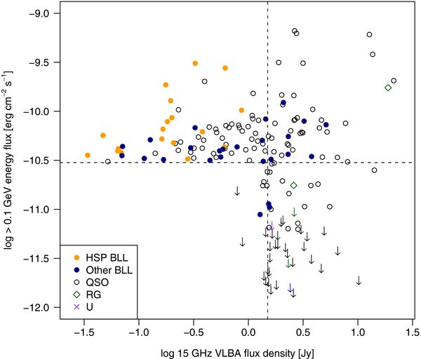
Figure 1. Plot of 11 month Fermi average >0.1 GeV energy flux vs. 15 GHz VLBA flux density for our joint AGN sample. The filled circles represent BL Lac objects, with the high-synchrotron peaked ones in orange and others in blue. The open circles represent quasars, the green diamonds radio galaxies, and the purple crosses optically unidentified objects. Upper limits on the γ-ray fluxes are indicated by arrows. All of the BL Lac objects are detected by the LAT, with the exception of J0006−0623. The vertical dashed line indicates the sample radio limit of 1.5 Jy, and the horizontal dashed line indicates the γ-ray limit of 3 × 10⁻¹¹ erg cm−2 s−1. Note that the radio flux density data correspond to either a median or “reference” epoch coincident with our VLBA observations (see Section 3.1), and do not necessarily coincide with the epoch of maximum radio flux density during the 11 month LAT period. Some AGNs in the bottom left quadrant thus have plotted flux densities below 1.5 Jy.
Download figure:
Standard image High-resolution image2.4. Selection Biases
We have assembled two complete samples of the brightest AGNs in the northern γ-ray and radio sky, as seen during the first 11 months of the Fermi mission. We list their general properties in Table 2. The optical redshifts and classifications are from the compilations of Lister et al. (2009a) and NED (see the Appendix for notes on individual sources). Note that we classify J0238+1636 as a quasar because of its occasional broad emission lines (Raiteri et al. 2007), and the presence of a break in its γ-ray spectrum that is characteristic of FSRQs (Abdo et al. 2010c). For the purposes of this paper, we have grouped two narrow-line Seyfert 1 galaxies J0948+0022 and J1504+1029 (Foschini 2011) with the quasar class.
Table 2. General Properties of AGNs in the Combined γ-Ray and Radio Samples
| J2000 | B1950 | 1FGL Name | Alias | z | Ref. | Opt. | SED | Ref. | Sample |
|---|---|---|---|---|---|---|---|---|---|
| (1) | (2) | (3) | (4) | (5) | (6) | (7) | (8) | (9) | (10) |
| J0006−0623 | 0003−066 | … | NRAO 005 | 0.3467 | Jones et al. (2009) | B | LSP | 1 | R |
| J0017−0512 | 0015−054 | J0017.4−0510 | PMN J0017−0512 | 0.226 | M. S. Shaw et al. (2011, in preparation) | Q | LSP | 2 | G |
| J0050−0929 | 0048−097 | J0050.6−0928 | PKS 0048−09 | … | … | B | ISP | 2 | B |
| J0108+0135 | 0106+013 | J0108.6+0135 | 4C +01.02 | 2.099 | Hewett et al. (1995) | Q | ISP | 1 | B |
| J0112+2244 | 0109+224 | J0112.0+2247 | S2 0109+22 | 0.265 | Healey et al. (2008) | B | ISP | 1 | G |
| J0112+3208 | 0110+318 | J0112.9+3207 | 4C +31.03 | 0.603 | Wills & Wills (1976) | Q | LSP | 11 | G |
| J0118−2141 | 0116−219 | J0118.7−2137 | OC −228 | 1.165 | Wright et al. (1983) | Q | LSP | 2 | G |
| J0120−2701 | 0118−272 | J0120.5−2700 | OC −230.4 | … | … | B | LSP | 2 | G |
| J0121+1149 | 0119+115 | … | PKS 0119+11 | 0.570 | Stickel et al. (1994) | Q | LSP | 1 | R |
| J0132−1654 | 0130−171 | J0132.6−1655 | OC −150 | 1.020 | Wright et al. (1983) | Q | LSP | 11 | B |
| J0136+3905 | 0133+388 | J0136.5+3905 | B3 0133+388 | … | … | B | HSP | 5 | G |
| J0136+4751 | 0133+476 | J0137.0+4751 | DA 55 | 0.859 | Lawrence et al. (1996) | Q | LSP | 1 | B |
| J0145−2733 | 0142−278 | J0144.9−2732 | OC −270 | 1.148 | Baker et al. (1999) | Q | LSP | 2 | G |
| J0205+3212 | 0202+319 | J0205.3+3217 | B2 0202+31 | 1.466 | Burbidge (1970) | Q | LSP | 1 | R |
| J0204−1701 | 0202−172 | J0205.0−1702 | PKS 0202−17 | 1.739 | Jones et al. (2009) | Q | LSP | 2 | R |
| J0217+7349 | 0212+735 | J0217.8+7353 | S5 0212+73 | 2.367 | Lawrence et al. (1996) | Q | LSP | 1 | R |
| J0217+0144 | 0215+015 | J0217.9+0144 | OD 026 | 1.715 | Boisse & Bergeron (1988) | Q | LSP | 1 | B |
| J0222+4302 | 0219+428 | J0222.6+4302 | 3C 66A | … | … | B | HSP | 5 | G |
| J0231+1322 | 0229+131 | … | 4C +13.14 | 2.059 | Osmer et al. (1994) | Q | LSP | 6 | R |
| J0237+2848 | 0234+285 | J0237.9+2848 | 4C 28.07 | 1.206 | M. S. Shaw et al. (2011, in preparation) | Q | LSP | 1 | B |
| J0238+1636 | 0235+164 | J0238.6+1637 | AO 0235+164 | 0.940 | Cohen et al. (1987) | Q | LSP | 1 | B |
| J0252−2219 | 0250−225 | J0252.8−2219 | OD −283 | 1.419 | M. S. Shaw et al. (2011, in preparation) | Q | LSP | 11 | G |
| J0303−2407 | 0301−243 | J0303.5−2406 | PKS 0301−243 | 0.260 | Falomo & Ulrich (2000) | B | HSP | 2 | G |
| J0316+0904 | 0313+085 | J0316.1+0904 | BZB J0316+0904 | … | … | B | HSP | 5 | G |
| J0319+4130 | 0316+413 | J0319.7+4130 | 3C 84 | 0.0176 | Strauss et al. (1992) | G | LSP | 4 | B |
| J0339−0146 | 0336−019 | J0339.2−0143 | CTA 26 | 0.852 | Wills & Lynds (1978) | Q | LSP | 1 | R |
| J0349−2102 | 0347−211 | J0349.9−2104 | OE −280 | 2.944 | Ellison et al. (2001) | Q | LSP | 2 | G |
| J0403+2600 | 0400+258 | … | CTD 026 | 2.109 | Schmidt (1977) | Q | … | … | R |
| J0423−0120 | 0420−014 | J0423.2−0118 | PKS 0420−01 | 0.9161 | Jones et al. (2009) | Q | LSP | 1 | B |
| J0433+0521 | 0430+052 | … | 3C 120 | 0.033 | Michel & Huchra (1988) | G | LSP | 1 | R |
| J0433+2905 | 0430+289 | J0433.5+2905 | BZB J0433+2905 | … | … | B | ISP | 5 | G |
| J0442−0017 | 0440−003 | J0442.7−0019 | NRAO 190 | 0.844 | Schmidt (1977) | Q | LSP | 6 | G |
| J0453−2807 | 0451−282 | J0453.2−2805 | OF −285 | 2.559 | Wright et al. (1983) | Q | LSP | 4 | B |
| J0457−2324 | 0454−234 | J0457.0−2325 | PKS 0454−234 | 1.003 | Stickel et al. (1989) | Q | LSP | 2 | B |
| J0507+6737 | 0502+675 | J0507.9+6738 | 1ES 0502+675 | 0.416 | Landt et al. (2002) | B | HSP | 2 | G |
| J0509+0541 | 0506+056 | J0509.3+0540 | TXS 0506+056 | … | … | B | HSP | 5 | G |
| J0530+1331 | 0528+134 | J0531.0+1331 | PKS 0528+134 | 2.070 | Hunter et al. (1993) | Q | LSP | 1 | B |
| J0532+0732 | 0529+075 | J0532.9+0733 | OG 050 | 1.254 | Sowards-Emmerd et al. (2005) | Q | LSP | 1 | B |
| J0608−1520 | 0605−153 | J0608.0−1521 | PMN J0608−1520 | 1.094 | M. S. Shaw et al. (2011, in preparation) | Q | LSP | 11 | G |
| J0609−1542 | 0607−157 | … | PKS 0607−15 | 0.3226 | Jones et al. (2009) | Q | LSP | 1 | R |
| J0612+4122 | 0609+413 | J0612.7+4120 | B3 0609+413 | … | … | B | … | … | G |
| J0630−2406 | 0628−240 | J0630.9−2406 | TXS 0628−240 | … | … | B | ISP | 4 | G |
| J0646+4451 | 0642+449 | … | OH 471 | 3.396 | Osmer et al. (1994) | Q | LSP | 1 | R |
| J0654+4514 | 0650+453 | J0654.3+4514 | B3 0650+453 | 0.928 | M. S. Shaw et al. (2011, in preparation) | Q | LSP | 2 | G |
| J0654+5042 | 0650+507 | J0654.4+5042 | GB6 J0654+5042 | 1.253 | M. S. Shaw et al. (2011, in preparation) | Q | LSP | 11 | G |
| J0713+1935 | 0710+196 | J0714.0+1935 | WB92 0711+1940 | 0.540 | M. S. Shaw et al. (2011, in preparation) | Q | LSP | 11 | G |
| J0719+3307 | 0716+332 | J0719.3+3306 | B2 0716+33 | 0.779 | White et al. (2000) | Q | LSP | 2 | G |
| J0721+7120 | 0716+714 | J0721.9+7120 | S5 0716+71 | 0.310 | Nilsson et al. (2008) | B | ISP | 5 | B |
| J0738+1742 | 0735+178 | J0738.2+1741 | O i 158 | … | … | B | LSP | 1 | G |
| J0739+0137 | 0736+017 | J0739.1+0138 | O i 061 | 0.1894 | Ho & Kim (2009) | Q | ISP | 1 | B |
| J0748+2400 | 0745+241 | … | PKS 0745+241 | 0.4092 | Abazajian et al. (2005) | Q | LSP | 4 | R |
| J0750+1231 | 0748+126 | J0750.6+1235 | O i 280 | 0.889 | Peterson et al. (1979) | Q | LSP | 1 | R |
| J0808−0751 | 0805−077 | J0808.2−0750 | PKS 0805−07 | 1.837 | White et al. (1988) | Q | LSP | 4 | B |
| J0818+4222 | 0814+425 | J0818.2+4222 | OJ 425 | … | … | B | LSP | 1 | B |
| J0825+0309 | 0823+033 | J0825.9+0309 | PKS 0823+033 | 0.506 | Stickel et al. (1993a) | B | LSP | 1 | R |
| J0830+2410 | 0827+243 | J0830.5+2407 | OJ 248 | 0.942 | M. S. Shaw et al. (2011, in preparation) | Q | LSP | 1 | R |
| J0836−2016 | 0834−201 | … | PKS 0834−20 | 2.752 | Fricke et al. (1983) | Q | … | … | R |
| J0841+7053 | 0836+710 | J0842.2+7054 | 4C +71.07 | 2.218 | McIntosh et al. (1999) | Q | LSP | 1 | R |
| J0854+2006 | 0851+202 | J0854.8+2006 | OJ 287 | 0.306 | Stickel et al. (1989) | B | LSP | 1 | B |
| J0909+0121 | 0906+015 | J0909.0+0126 | 4C +01.24 | 1.0256 | M. S. Shaw et al. (2011, in preparation) | Q | ISP | 1 | B |
| J0920+4441 | 0917+449 | J0920.9+4441 | S4 0917+44 | 2.189 | Abazajian et al. (2004) | Q | LSP | 6 | B |
| J0927+3902 | 0923+392 | … | 4C +39.25 | 0.695 | Abazajian et al. (2005) | Q | LSP | 1 | R |
| J0948+4039 | 0945+408 | … | 4C +40.24 | 1.249 | Abazajian et al. (2005) | Q | LSP | 1 | R |
| J0948+0022 | 0946+006 | J0949.0+0021 | PMN J0948+0022 | 0.585 | Abazajian et al. (2004) | Q | LSP | 2 | G |
| J0957+5522 | 0954+556 | J0957.7+5523 | 4C +55.17 | 0.8993 | M. S. Shaw et al. (2011, in preparation) | Q | LSP | 6 | G |
| J0958+6533 | 0954+658 | J1000.1+6539 | S4 0954+65 | 0.367 | Rector & Stocke (2001) | B | LSP | 5 | R |
| J1012+2439 | 1009+245 | J1012.7+2440 | GB6 J1012+2439 | 1.805 | M. S. Shaw et al. (2011, in preparation) | Q | … | … | G |
| J1015+4926 | 1011+496 | J1015.1+4927 | 7C 1011+4941 | 0.212 | Albert et al. (2007) | B | HSP | 2 | G |
| J1016+0513 | 1013+054 | J1016.1+0514 | TXS 1013+054 | 1.713 | Abazajian et al. (2004) | Q | … | … | G |
| J1037+5711 | 1034+574 | J1037.7+5711 | GB6 J1037+5711 | … | … | B | ISP | 5 | G |
| J1037−2934 | 1034−293 | … | PKS 1034−293 | 0.312 | Scarpa & Falomo (1997) | Q | LSP | 10 | R |
| J1038+0512 | 1036+054 | … | PKS 1036+054 | 0.473 | Healey et al. (2008) | Q | LSP | 1 | R |
| J1058+0133 | 1055+018 | J1058.4+0134 | 4C +01.28 | 0.888 | M. S. Shaw et al. (2011, in preparation) | Q | LSP | 1 | B |
| J1058+5628 | 1055+567 | J1058.6+5628 | 7C 1055+5644 | 0.143 | Abazajian et al. (2004) | B | HSP | 5 | G |
| J1104+3812 | 1101+384 | J1104.4+3812 | Mrk 421 | 0.0308 | Ulrich et al. (1975) | B | HSP | 2 | G |
| J1121−0553 | 1118−056 | J1121.5−0554 | PKS 1118−05 | 1.297 | Drinkwater et al. (1997) | Q | LSP | 11 | G |
| J1127−1857 | 1124−186 | J1126.8−1854 | PKS 1124−186 | 1.048 | Drinkwater et al. (1997) | Q | ISP | 1 | R |
| J1130−1449 | 1127−145 | J1130.2−1447 | PKS 1127−14 | 1.184 | Wilkes (1986) | Q | LSP | 2 | B |
| J1159+2914 | 1156+295 | J1159.4+2914 | 4C +29.45 | 0.7246 | M. S. Shaw et al. (2011, in preparation) | Q | ISP | 1 | B |
| J1215−1731 | 1213−172 | … | PKS 1213−17 | … | … | U | LSP | 1 | R |
| J1217+3007 | 1215+303 | J1217.7+3007 | ON 325 | 0.130 | Akiyama et al. (2003) | B | HSP | 5 | G |
| J1221+3010 | 1218+304 | J1221.3+3008 | B2 1218+30 | 0.1836 | Adelman-McCarthy et al. (2008) | B | HSP | 9 | G |
| J1221+2813 | 1219+285 | J1221.5+2814 | W Comae | … | … | B | ISP | 5 | G |
| J1224+2122 | 1222+216 | J1224.7+2121 | 4C +21.35 | 0.434 | Schneider et al. (2010) | Q | LSP | 6 | G |
| J1229+0203 | 1226+023 | J1229.1+0203 | 3C 273 | 0.1583 | Strauss et al. (1992) | Q | LSP | 1 | B |
| J1230+1223 | 1228+126 | J1230.8+1223 | M87 | 0.00436 | Smith et al. (2000) | G | LSP | 7 | R |
| J1239+0443 | 1236+049 | J1239.5+0443 | BZQ J1239+0443 | 1.761 | M. S. Shaw et al. (2011, in preparation) | Q | LSP | 11 | G |
| J1246−2547 | 1244−255 | J1246.7−2545 | PKS 1244−255 | 0.633 | Savage et al. (1976) | Q | LSP | 2 | G |
| J1248+5820 | 1246+586 | J1248.2+5820 | PG 1246+586 | … | … | B | HSP | 5 | G |
| J1256−0547 | 1253−055 | J1256.2−0547 | 3C 279 | 0.536 | Marziani et al. (1996) | Q | LSP | 1 | B |
| J1303+2433 | 1300+248 | J1303.0+2433 | VIPS 0623 | … | … | B | … | … | G |
| J1310+3220 | 1308+326 | J1310.6+3222 | OP 313 | 0.9973 | M. S. Shaw et al. (2011, in preparation) | Q | ISP | 1 | B |
| J1332−0509 | 1329−049 | J1331.9−0506 | OP −050 | 2.150 | Thompson et al. (1990) | Q | LSP | 2 | G |
| J1332−1256 | 1329−126 | J1332.6−1255 | PMN J1332−1256 | 1.492 | M. S. Shaw et al. (2011, in preparation) | Q | … | … | G |
| J1337−1257 | 1334−127 | J1337.7−1255 | PKS 1335−127 | 0.539 | Stickel et al. (1993b) | Q | LSP | 1 | B |
| J1344−1723 | 1341−171 | J1344.2−1723 | PMN J1344−1723 | 2.506 | M. S. Shaw et al. (2011, in preparation) | Q | … | … | G |
| J1427+2348 | 1424+240 | J1426.9+2347 | OQ +240 | … | … | B | HSP | 5 | G |
| J1436+6336 | 1435+638 | … | VIPS 0792 | 2.066 | McIntosh et al. (1999) | Q | LSP | 4 | R |
| J1504+1029 | 1502+106 | J1504.4+1029 | OR 103 | 1.8385 | Adelman-McCarthy et al. (2008) | Q | LSP | 1 | B |
| J1512−0905 | 1510−089 | J1512.8−0906 | PKS 1510−08 | 0.360 | Thompson et al. (1990) | Q | LSP | 1 | B |
| J1516+1932 | 1514+197 | J1516.9+1928 | PKS 1514+197 | … | … | B | LSP | 5 | R |
| J1517−2422 | 1514−241 | J1517.8−2423 | AP Librae | 0.049 | Jones et al. (2009) | B | LSP | 2 | B |
| J1522+3144 | 1520+319 | J1522.1+3143 | B2 1520+31 | 1.484 | M. S. Shaw et al. (2011, in preparation) | Q | LSP | 2 | G |
| J1542+6129 | 1542+616 | J1542.9+6129 | GB6 J1542+6129 | … | … | B | ISP | 5 | G |
| J1549+0237 | 1546+027 | J1549.3+0235 | PKS 1546+027 | 0.414 | Abazajian et al. (2004) | Q | LSP | 1 | R |
| J1550+0527 | 1548+056 | J1550.7+0527 | 4C +05.64 | 1.417 | M. S. Shaw et al. (2011, in preparation) | Q | LSP | 1 | R |
| J1553+1256 | 1551+130 | J1553.4+1255 | OR +186 | 1.308 | Schneider et al. (2010) | Q | … | … | G |
| J1555+1111 | 1553+113 | J1555.7+1111 | PG 1553+113 | … | … | B | HSP | 5 | G |
| J1613+3412 | 1611+343 | J1613.5+3411 | DA 406 | 1.40 | M. S. Shaw et al. (2011, in preparation) | Q | LSP | 1 | R |
| J1625−2527 | 1622−253 | J1625.7−2524 | PKS 1622−253 | 0.786 | di Serego-Alighieri et al. (1994) | Q | LSP | 2 | B |
| J1635+3808 | 1633+382 | J1635.0+3808 | 4C +38.41 | 1.813 | M. S. Shaw et al. (2011, in preparation) | Q | LSP | 1 | B |
| J1638+5720 | 1637+574 | … | OS 562 | 0.751 | Marziani et al. (1996) | Q | ISP | 1 | R |
| J1640+3946 | 1638+398 | … | NRAO 512 | 1.666 | Stickel et al. (1989) | Q | LSP | 1 | R |
| J1642+3948 | 1641+399 | J1642.5+3947 | 3C 345 | 0.593 | Marziani et al. (1996) | Q | ISP | 1 | B |
| J1642+6856 | 1642+690 | … | 4C +69.21 | 0.751 | Lawrence et al. (1996) | Q | LSP | 6 | R |
| J1653+3945 | 1652+398 | J1653.9+3945 | Mrk 501 | 0.0337 | Stickel et al. (1993a) | B | HSP | 2 | G |
| J1658+0741 | 1655+077 | … | PKS 1655+077 | 0.621 | Wilkes (1986) | Q | LSP | 1 | R |
| J1700+6830 | 1700+685 | J1700.1+6830 | TXS 1700+685 | 0.301 | Henstock et al. (1997) | Q | LSP | 4 | G |
| J1719+1745 | 1717+178 | J1719.2+1745 | OT 129 | 0.137 | Sowards-Emmerd et al. (2005) | B | LSP | 5 | G |
| J1725+1152 | 1722+119 | J1725.0+1151 | 1H 1720+117 | … | … | B | HSP | 5 | G |
| J1727+4530 | 1726+455 | J1727.3+4525 | S4 1726+45 | 0.717 | Henstock et al. (1997) | Q | LSP | 1 | R |
| J1733−1304 | 1730−130 | J1733.0−1308 | NRAO 530 | 0.902 | Junkkarinen (1984) | Q | LSP | 1 | B |
| J1734+3857 | 1732+389 | J1734.4+3859 | OT 355 | 0.975 | M. S. Shaw et al. (2011, in preparation) | Q | LSP | 11 | G |
| J1740+5211 | 1739+522 | J1740.0+5209 | 4C +51.37 | 1.379 | Walsh et al. (1984) | Q | LSP | 1 | G |
| J1743−0350 | 1741−038 | … | PKS 1741−03 | 1.054 | White et al. (1988) | Q | LSP | 1 | R |
| J1751+0939 | 1749+096 | J1751.5+0937 | 4C +09.57 | 0.322 | Stickel et al. (1988) | B | LSP | 1 | B |
| J1753+2848 | 1751+288 | … | B2 1751+28 | 1.118 | Healey et al. (2008) | Q | LSP | 1 | R |
| J1801+4404 | 1800+440 | … | S4 1800+44 | 0.663 | Walsh & Carswell (1982) | Q | ISP | 1 | R |
| J1800+7828 | 1803+784 | J1800.4+7827 | S5 1803+784 | 0.6797 | Lawrence et al. (1996) | B | LSP | 1 | B |
| J1806+6949 | 1807+698 | J1807.0+6945 | 3C 371 | 0.051 | de Grijp et al. (1992) | B | ISP | 1 | B |
| J1824+5651 | 1823+568 | J1824.0+5651 | 4C +56.27 | 0.664 | M. S. Shaw et al. (2011, in preparation) | B | LSP | 1 | B |
| J1829+4844 | 1828+487 | J1829.8+4845 | 3C 380 | 0.692 | Lawrence et al. (1996) | Q | LSP | 4 | R |
| J1842+6809 | 1842+681 | … | GB6 J1842+6809 | 0.472 | Xu et al. (1994) | Q | … | … | R |
| J1848+3219 | 1846+322 | J1848.5+3224 | B2 1846+32A | 0.798 | Sowards-Emmerd et al. (2005) | Q | LSP | 2 | G |
| J1849+6705 | 1849+670 | J1849.3+6705 | S4 1849+67 | 0.657 | Stickel & Kuehr (1993) | Q | LSP | 1 | B |
| J1903+5540 | 1902+556 | J1903.0+5539 | TXS 1902+556 | … | … | B | ISP | 5 | G |
| J1911−2006 | 1908−201 | J1911.2−2007 | PKS B1908−201 | 1.119 | Halpern et al. (2003) | Q | LSP | 2 | B |
| J1923−2104 | 1920−211 | J1923.5−2104 | OV −235 | 0.874 | Halpern et al. (2003) | Q | LSP | 2 | B |
| J1924−2914 | 1921−293 | J1925.2−2919 | PKS B1921−293 | 0.3526 | Jones et al. (2009) | Q | LSP | 10 | R |
| J1927+7358 | 1928+738 | … | 4C +73.18 | 0.302 | Marziani et al. (1996) | Q | ISP | 1 | R |
| J1954−1123 | 1951−115 | J1954.8−1124 | TXS 1951−115 | 0.683 | M. S. Shaw et al. (2011, in preparation) | Q | LSP | 11 | G |
| J1955+5131 | 1954+513 | … | … | 1.223 | Lawrence et al. (1996) | Q | LSP | 7 | R |
| J2000−1748 | 1958−179 | J2000.9−1749 | PKS 1958−179 | 0.652 | Abdo et al. (2010d) | Q | LSP | 1 | B |
| J1959+6508 | 1959+650 | J2000.0+6508 | 1ES 1959+650 | 0.047 | Schachter et al. (1993) | B | HSP | 2 | G |
| J2011−1546 | 2008−159 | … | PKS 2008−159 | 1.180 | Peterson et al. (1979) | Q | ISP | 1 | R |
| J2022+6136 | 2021+614 | … | OW 637 | 0.227 | Hewitt & Burbidge (1991) | G | LSP | 1 | R |
| J2025−0735 | 2022−077 | J2025.6−0735 | PKS 2023−07 | 1.388 | Drinkwater et al. (1997) | Q | LSP | 2 | G |
| J2031+1219 | 2029+121 | J2031.5+1219 | PKS 2029+121 | 1.213 | M. S. Shaw et al. (2011, in preparation) | Q | LSP | 11 | R |
| J2123+0535 | 2121+053 | … | PKS 2121+053 | 1.941 | Steidel & Sargent (1991) | Q | ISP | 1 | R |
| J2131−1207 | 2128−123 | … | PKS 2128−12 | 0.501 | Searle & Bolton (1968) | Q | ISP | 1 | R |
| J2134−0153 | 2131−021 | J2134.0−0203 | 4C−02.81 | 1.284 | Abdo et al. (2010d) | Q | LSP | 1 | R |
| J2136+0041 | 2134+004 | … | PKS 2134+004 | 1.932 | Osmer et al. (1994) | Q | LSP | 1 | R |
| J2139+1423 | 2136+141 | … | OX 161 | 2.427 | Wills & Wills (1974) | Q | LSP | 7 | R |
| J2143+1743 | 2141+175 | J2143.4+1742 | OX 169 | 0.2107 | Ho & Kim (2009) | Q | ISP | 2 | G |
| J2147+0929 | 2144+092 | J2147.2+0929 | PKS 2144+092 | 1.113 | White et al. (1988) | Q | LSP | 2 | G |
| J2148+0657 | 2145+067 | J2148.5+0654 | 4C +06.69 | 0.999 | Steidel & Sargent (1991) | Q | LSP | 1 | R |
| J2158−1501 | 2155−152 | J2157.9−1503 | PKS 2155−152 | 0.672 | White et al. (1988) | Q | LSP | 1 | R |
| J2202+4216 | 2200+420 | J2202.8+4216 | BL Lac | 0.0686 | Vermeulen et al. (1995) | B | LSP | 1 | B |
| J2203+1725 | 2201+171 | J2203.5+1726 | PKS 2201+171 | 1.076 | Smith et al. (1977) | Q | ISP | 1 | G |
| J2203+3145 | 2201+315 | … | 4C +31.63 | 0.2947 | Marziani et al. (1996) | Q | ISP | 1 | R |
| J2218−0335 | 2216−038 | … | PKS 2216−03 | 0.901 | Lynds (1967) | Q | ISP | 1 | R |
| J2225−0457 | 2223−052 | J2225.8−0457 | 3C 446 | 1.404 | Wright et al. (1983) | Q | LSP | 4 | B |
| J2229−0832 | 2227−088 | J2229.7−0832 | PHL 5225 | 1.5595 | Abazajian et al. (2004) | Q | LSP | 1 | B |
| J2232+1143 | 2230+114 | J2232.5+1144 | CTA 102 | 1.037 | Falomo et al. (1994) | Q | ISP | 1 | B |
| J2236−1433 | 2233−148 | J2236.4−1432 | OY −156 | … | … | B | LSP | 11 | G |
| J2236+2828 | 2234+282 | J2236.2+2828 | CTD 135 | 0.795 | Jackson & Browne (1991) | Q | LSP | 7 | G |
| J2243+2021 | 2241+200 | J2244.0+2021 | RGB J2243+203 | … | … | B | ISP | 5 | G |
| J2246−1206 | 2243−123 | … | PKS 2243−123 | 0.632 | Browne et al. (1975) | Q | ISP | 1 | R |
| J2250−2806 | 2247−283 | J2250.8−2809 | PMN J2250−2806 | 0.525 | M. S. Shaw et al. (2011, in preparation) | Q | LSP | 11 | G |
| J2253+1608 | 2251+158 | J2253.9+1608 | 3C 454.3 | 0.859 | Jackson & Browne (1991) | Q | ISP | 1 | B |
| J2327+0940 | 2325+093 | J2327.7+0943 | OZ 042 | 1.841 | M. S. Shaw et al. (2011, in preparation) | Q | LSP | 2 | B |
| J2331−2148 | 2328−221 | J2331.0−2145 | PMN J2331−2148 | 0.563 | M. S. Shaw et al. (2011, in preparation) | Q | … | … | G |
| J2348−1631 | 2345−167 | J2348.0−1629 | PKS 2345−16 | 0.576 | Tadhunter et al. (1993) | Q | LSP | 1 | R |
Notes. Column 1: IAU name (J2000), Column 2: IAU name (B1950), Column 3: 1FGL catalog name, Column 4: other name, Column 5: redshift, Column 6: literature reference for redshift, Column 7: optical classification, where B, BL Lac; Q, quasar; G, radio galaxy; and U, unidentified, Column 8: spectral energy distribution class, where HSP, high spectral peaked; ISP, intermediate spectral peaked; and LSP, low spectral peaked. Column 9: literature reference for SED data, where (1) Chang 2010; (2) Abdo et al. 2010e; (3) Abdo et al. 2010a; (4) Meyer et al. 2011; (5) Nieppola et al. 2006; (6) Nieppola et al. (2008); (7) Aatrokoski 2011; (8) Tavecchio et al. 2010; (9) Rüger et al. 2010; (10) Impey & Neugebauer 1988; (11) 2LAC catalog, Ackermann et al. 2011; Column 10: sample membership, where G, 1FM γ-ray selected sample; R, 1FM-matching radio sample; B, in both samples.
The SED data are taken mainly from Chang (2010), Abdo et al. (2010e), and other papers in the literature as indicated in Column 8. We use the following nomenclature for high-, intermediate-, and low-synchrotron peaked blazars: LSP <1014, 1014 < ISP <1015, and HSP >1015, where the values refer to the synchrotron SED peak frequency νs in Hertz.
Although our γ-ray and radio selections are both made on the basis of compact beamed jet emission, there is only a 28% overlap in the two samples. This is perhaps lower than might be expected, given the strong correlations previously seen between the 1LAC catalog and flat-spectrum radio sources (Abdo et al. 2010d). As we will discuss in Section 3.3, however, this is mainly a consequence of the wide range of γ-ray loudness in the bright blazar population. There is also some likelihood that any particular AGN will not have a LAT association because it happens to lie in a confused region that contains several bright γ-ray sources, or has a high diffuse γ-ray background. The latter case is less likely to occur however for the bright non-Galactic-plane sources we are considering. We have carefully examined our candidate list and found only one possible case of a missed association: 1FGL J1642.5+3947. Recent analysis by the LAT team (Schinzel et al. 2010) has led us to associate this source with the FSRQ J1642+3948 (3C 345).
The nature of our γ-ray sample selection differs from that of our radio sample, since it uses average fluxes instead of maximum measured flux densities, and it spans a wide energy band compared to the radio. It is thus more sensitive to the shapes of the AGN SEDs, which can have curvature and breaks within the LAT detector band. The spectral response function of the LAT detector and its favoritism toward harder sources causes some selection bias toward faint HSP AGNs (Abdo et al. 2010a). We note, however, that the sources in our 1FM sample are selected well above the instrument sensitivity level of the LAT detector and should be devoid of biases related to threshold effects.
The above selection biases do not have a large impact on the analysis presented in this paper, since our primary goal is to identify broad statistical trends between the γ-ray emission and radio jet properties. For this purpose a representative blazar sample that spans a wide range of SED peak frequency and γ-ray loudness is appropriate. Future studies using more extensive Fermi data will address these issues in considerably more detail, with better statistics. These will be needed for accurate determination of the blazar γ-ray luminosity function for different redshift ranges and optical sub-classes.
3. OBSERVATIONAL DATA
3.1. Radio Flux Density Data
We list the radio flux density data for our sample in Table 3. For each AGN we selected a VLBA “reference” epoch, which was chosen to be the closest MOJAVE VLBA observation to the end of the initial 11 month Fermi period. In the case of 41 sources, no VLBA data were available within this period, so we used the first available MOJAVE VLBA epoch following this period. The latter epoch dates ranged from 2009 July 23 to 2010 November 29. We list the reference epoch dates and total 15 GHz VLBA flux densities in Columns 3 and 4, respectively. In Column 5, we list the median single dish flux density from OVRO at 15 GHz (or 14.5 GHz at UMRAO as indicated) during the same 11 month period (Richards et al. 2011; Aller et al. 2003).
Table 3. Flux Data
| J2000 | B1950 | VLBA | VLBA | Single Dish | Arcsecond | Gr |
|---|---|---|---|---|---|---|
| Name | Name | Epoch | Total | Median | Emission | |
| (Jy) | (Jy) | (Jy) | ||||
| (1) | (2) | (3) | (4) | (5) | (6) | (7) |
| J0006−0623 | 0003−066 | 2009 May 2 | 2.50 | 2.41 | … | <6.7 |
| J0017−0512 | 0015−054 | 2009 Jul 5 | 0.29 | 0.32 | … | 972 |
| J0050−0929 | 0048−097 | 2008 Oct 3 | 1.09 | 1.34 | … | 344 |
| J0108+0135 | 0106+013 | 2009 Jun 25 | 2.77 | 2.66 | … | 1174 |
| J0112+2244 | 0109+224 | 2009 Jul 5 | 0.48 | 0.79 | … | 489 |
| J0112+3208 | 0110+318 | 2009 Jun 3 | 0.70 | … | … | 1332 |
| J0118−2141 | 0116−219 | 2009 Jul 23 | 0.70 | … | … | 1047 |
| J0120−2701 | 0118−272 | 2009 Dec 26 | 0.56 | … | … | 529 |
| J0121+1149 | 0119+115 | 2009 Jun 15 | 3.57 | 3.76 | … | <9.9 |
| J0132−1654 | 0130−171 | 2009 Oct 27 | 2.02 | 2.02 | … | 352 |
| J0136+3906 | 0133+388 | 2010 Nov 29 | 0.05 | … | … | 9763 |
| J0136+4751 | 0133+476 | 2009 Jun 25 | 4.44 | 3.87 | … | 415 |
| J0145−2733 | 0142−278 | 2009 Dec 26 | 0.95 | … | … | 972 |
| J0205+3212 | 0202+319 | 2008 Aug 25 | 3.17 | 3.26 | … | 106 |
| J0204−1701 | 0202−172 | 2009 Jul 5 | 1.45 | 1.47 | … | 370 |
| J0217+7349 | 0212+735 | 2008 Sep 12 | 3.78 | 3.72 | … | 296 |
| J0217+0144 | 0215+015 | 2008 Nov 19 | 2.00 | 1.53 | … | 788 |
| J0222+4302 | 0219+428 | 2009 Jun 15 | 0.60 | 0.86 | 0.25 | 3827 |
| J0231+1322 | 0229+131 | 2010 Oct 25 | 1.90 | 1.57 | … | <51 |
| J0237+2848 | 0234+285 | 2009 Jun 25 | 2.54 | 3.14 | … | 427 |
| J0238+1636 | 0235+164 | 2009 Mar 25 | 3.08 | 3.15 | … | 1396 |
| J0252−2219 | 0250−225 | 2009 Mar 25 | 0.51 | … | … | 2677 |
| J0303−2407 | 0301−243 | 2010 Mar 1 | 0.21 | … | … | 1933 |
| J0316+0904 | 0313+085 | 2010 Nov 20 | 0.06 | … | … | 4960 |
| J0319+4130 | 0316+413 | 2009 May 28 | 19.40 | 18.91 | … | 63 |
| J0339−0146 | 0336−019 | 2009 May 2 | 2.36 | 2.35 | … | 104 |
| J0349−2102 | 0347−211 | 2009 Jul 5 | 0.62 | … | … | 3981 |
| J0403+2600 | 0400+258 | 2010 Oct 15 | 1.85 | 1.85 | … | <75 |
| J0423−0120 | 0420−014 | 2009 Jul 5 | 6.29 | 4.45 | … | 254 |
| J0433+0521 | 0430+052 | 2009 Jul 5 | 2.69 | 3.18 | 0.56 | <27 |
| J0433+2905 | 0430+289 | 2009 Jul 23 | 0.31 | 0.30 | … | 1280 |
| J0442−0017 | 0440−003 | 2009 May 28 | 1.26 | 1.24 | … | 1050 |
| J0453−2807 | 0451−282 | 2009 Aug 19 | 1.71 | … | … | 1201 |
| J0457−2324 | 0454−234 | 2009 Jun 25 | 1.99 | 1.89a | … | 2566 |
| J0507+6737 | 0502+675 | 2010 Nov 20 | 0.05 | 0.03 | … | 9048 |
| J0509+0541 | 0506+056 | 2009 Jun 3 | 0.59 | 0.60 | … | 646 |
| J0530+1331 | 0528+134 | 2009 Mar 25 | 2.86 | 2.98 | … | 838 |
| J0532+0732 | 0529+075 | 2009 May 2 | 1.47 | 1.42 | … | 608 |
| J0608−1520 | 0605−153 | 2010 Mar 1 | 0.20 | 0.21 | … | 4471 |
| J0609−1542 | 0607−157 | 2009 Jun 25 | 5.17 | 4.92 | … | <12 |
| J0612+4122 | 0609+413 | 2009 Dec 26 | 0.22 | 0.28 | … | 1022 |
| J0630−2406 | 0628−240 | 2010 Nov 29 | 0.07 | … | … | 4221 |
| J0646+4451 | 0642+449 | 2009 May 28 | 3.62 | 3.43 | … | <57 |
| J0654+4514 | 0650+453 | 2009 Jun 25 | 0.38 | 0.50 | … | 2063 |
| J0654+5042 | 0650+507 | 2009 Jul 5 | 0.20 | 0.23 | … | 2805 |
| J0713+1935 | 0710+196 | 2009 Aug 19 | 0.44 | … | … | 1885 |
| J0719+3307 | 0716+332 | 2009 Feb 25 | 0.57 | 0.58 | … | 1193 |
| J0721+7120 | 0716+714 | 2009 Jun 15 | 1.20 | 2.09 | … | 534 |
| J0738+1742 | 0735+178 | 2009 Jun 25 | 0.62 | 0.74 | 0.19 | 629 |
| J0739+0137 | 0736+017 | 2009 Jul 5 | 1.20 | 1.33 | 0.20 | 328 |
| J0748+2400 | 0745+241 | 2010 Oct 25 | 1.15 | 1.54 | … | <16 |
| J0750+1231 | 0748+126 | 2009 Feb 25 | 4.30 | 4.33 | … | 70 |
| J0808−0751 | 0805−077 | 2009 Jun 25 | 1.91 | 1.08 | … | 1835 |
| J0818+4222 | 0814+425 | 2009 May 28 | 1.68 | 1.44 | … | 523 |
| J0825+0309 | 0823+033 | 2009 Jul 5 | 0.98 | 1.53 | … | 70 |
| J0830+2410 | 0827+243 | 2008 Nov 19 | 1.53 | 1.49 | … | 353 |
| J0836−2016 | 0834−201 | 2009 Mar 25 | 2.07 | … | 0.65 | <118 |
| J0841+7053 | 0836+710 | 2009 May 2 | 1.58 | 1.57 | … | 1028 |
| J0854+2006 | 0851+202 | 2009 May 28 | 4.67 | 3.78 | … | 88 |
| J0909+0121 | 0906+015 | 2009 May 28 | 1.54 | 1.35 | … | 781 |
| J0920+4441 | 0917+449 | 2009 Jun 25 | 2.12 | 2.02 | … | 2154 |
| J0927+3902 | 0923+392 | 2009 Jul 5 | 10.86 | 10.18 | … | <2.4 |
| J0948+4039 | 0945+408 | 2009 Jun 3 | 1.69 | 1.76 | … | <44 |
| J0948+0022 | 0946+006 | 2009 May 28 | 0.44 | 0.24 | … | 2901 |
| J0957+5522 | 0954+556 | 2009 Mar 25 | 0.15 | 1.19 | 0.96 | 5909 |
| J0958+6533 | 0954+658 | 2009 Jul 5 | 1.34 | 1.28 | … | 74 |
| J1012+2439 | 1009+245 | 2010 Nov 29 | 0.05 | 0.05 | … | 14584 |
| J1015+4926 | 1011+496 | 2009 May 2 | 0.20 | 0.28 | 0.08 | 3431 |
| J1016+0513 | 1013+054 | 2009 Jun 15 | 0.66 | 0.62 | … | 2730 |
| J1037+5711 | 1034+574 | 2010 Mar 1 | 0.11 | 0.17 | … | 1649 |
| J1037−2934 | 1034−293 | 2010 Oct 15 | 1.44 | … | … | <13 |
| J1038+0512 | 1036+054 | 2008 Oct 3 | 1.49 | 1.38 | … | <17 |
| J1058+0133 | 1055+018 | 2008 Aug 25 | 4.32 | 4.65 | … | 265 |
| J1058+5628 | 1055+567 | 2009 Aug 19 | 0.18 | 0.17 | … | 3011 |
| J1104+3812 | 1101+384 | 2009 Jun 25 | 0.33 | 0.44 | 0.11 | 6456 |
| J1121−0553 | 1118−056 | 2009 Jun 15 | 0.48 | … | … | 1495 |
| J1127−1857 | 1124−186 | 2009 May 2 | 1.74 | 1.64 | … | 334 |
| J1130−1449 | 1127−145 | 2009 Jul 5 | 2.33 | 2.27 | … | 528 |
| J1159+2914 | 1156+295 | 2009 Jun 3 | 2.18 | 3.07 | … | 280 |
| J1215−1731 | 1213−172 | 2008 Sep 12 | 1.75 | 1.80 | 0.16 | <41 |
| J1217+3007 | 1215+303 | 2009 Jun 15 | 0.36 | 0.38 | … | 1223 |
| J1221+3010 | 1218+304 | 2010 Nov 20 | 0.07 | … | … | 4114 |
| J1221+2813 | 1219+285 | 2009 May 28 | 0.33 | 0.40 | 0.07 | 1837 |
| J1224+2122 | 1222+216 | 2009 May 28 | 1.01 | 1.15 | 0.13 | 359 |
| J1229+0203 | 1226+023 | 2009 Jun 25 | 24.38 | 27.84 | 6.58 | 83 |
| J1230+1223 | 1228+126 | 2009 Jul 5 | 2.51 | 26.30 | 23.71 | 45 |
| J1239+0443 | 1236+049 | 2009 Jun 3 | 0.36 | 0.38 | … | 2926 |
| J1246−2547 | 1244−255 | 2009 Jun 15 | 1.10 | … | … | 970 |
| J1248+5820 | 1246+586 | 2009 Oct 27 | 0.12 | 0.16 | … | 2929 |
| J1256−0547 | 1253−055 | 2009 Jun 25 | 12.01 | 13.65 | … | 328 |
| J1303+2433 | 1300+248 | 2010 Nov 13 | 0.11 | 0.28 | … | 1049 |
| J1310+3220 | 1308+326 | 2009 Jun 3 | 2.22 | 1.75 | … | 705 |
| J1332−0509 | 1329−049 | 2009 Jul 5 | 1.12 | 0.99 | … | 3117 |
| J1332−1256 | 1329−126 | 2010 Mar 1 | 0.35 | … | … | 3917 |
| J1337−1257 | 1334−127 | 2009 Jun 25 | 6.59 | 6.51 | … | 66 |
| J1344−1723 | 1341−171 | 2009 Jun 25 | 0.33 | 0.39 | … | 3486 |
| J1427+2348 | 1424+240 | 2009 Jun 25 | 0.18 | 0.26 | 0.06 | 5450 |
| J1436+6336 | 1435+638 | 2010 Jul 12 | 1.54 | 1.50 | … | <41 |
| J1504+1029 | 1502+106 | 2009 Mar 25 | 3.15 | 2.65 | … | 5965 |
| J1512−0905 | 1510−089 | 2009 Jul 5 | 3.98 | 2.75 | … | 2335 |
| J1516+1932 | 1514+197 | 2010 Sep 27 | 0.90 | 1.56 | … | 64 |
| J1517−2422 | 1514−241 | 2009 Jun 3 | 2.32 | … | … | 168 |
| J1522+3144 | 1520+319 | 2009 Jun 15 | 0.42 | 0.40 | … | 12312 |
| J1542+6129 | 1542+616 | 2010 Nov 29 | 0.14 | 0.13 | … | 3628 |
| J1549+0237 | 1546+027 | 2009 Jun 25 | 1.79 | 1.72 | … | 191 |
| J1550+0527 | 1548+056 | 2009 Jan 30 | 2.64 | 2.83 | … | 56 |
| J1553+1256 | 1551+130 | 2009 Jun 3 | 0.67 | 0.67 | … | 2032 |
| J1555+1111 | 1553+113 | 2009 Jun 15 | 0.15 | 0.18 | … | 8397 |
| J1613+3412 | 1611+343 | 2009 May 2 | 2.81 | 2.83 | … | 46 |
| J1625−2527 | 1622−253 | 2009 Oct 27 | 2.32 | … | … | 286 |
| J1635+3808 | 1633+382 | 2009 May 2 | 2.88 | 2.80 | … | 933 |
| J1638+5720 | 1637+574 | 2009 Mar 25 | 1.81 | 1.80 | … | <13 |
| J1640+3946 | 1638+398 | 2009 May 28 | 0.78 | 0.79 | … | <418 |
| J1642+3948 | 1641+399 | 2009 Jul 5 | 9.14 | 7.72 | … | 130 |
| J1642+6856 | 1642+690 | 2008 Nov 26 | 3.84 | 4.62 | … | <7.3 |
| J1653+3945 | 1652+398 | 2009 Jun 15 | 0.87 | 1.17 | 0.30 | 812 |
| J1658+0741 | 1655+077 | 2009 Jul 5 | 1.85 | … | … | <29 |
| J1700+6830 | 1700+685 | 2009 Jul 5 | 0.25 | 0.30 | … | 1201 |
| J1719+1745 | 1717+178 | 2009 Jul 5 | 0.58 | 0.58 | … | 533 |
| J1725+1152 | 1722+119 | 2010 Nov 20 | 0.07 | 0.07 | … | 5390 |
| J1727+4530 | 1726+455 | 2008 Aug 25 | 1.02 | 1.39 | … | 215 |
| J1733−1304 | 1730−130 | 2009 Jun 25 | 4.00 | 4.74 | … | 113 |
| J1734+3857 | 1732+389 | 2009 Dec 26 | 0.97 | 0.88 | … | 1097 |
| J1740+5211 | 1739+522 | 2008 Aug 25 | 0.94 | 1.16 | … | 1504 |
| J1743−0350 | 1741−038 | 2008 Nov 19 | 3.26 | 3.02 | … | <33 |
| J1751+0939 | 1749+096 | 2009 Jun 3 | 4.20 | 5.13 | … | 136 |
| J1753+2848 | 1751+288 | 2009 Jun 25 | 1.48 | 1.57 | … | <44 |
| J1801+4404 | 1800+440 | 2008 Aug 25 | 1.32 | 1.44 | … | <52 |
| J1800+7828 | 1803+784 | 2009 Mar 25 | 2.40 | 2.31 | … | 212 |
| J1806+6949 | 1807+698 | 2009 Jul 5 | 1.37 | 1.60 | 0.23 | 163 |
| J1824+5651 | 1823+568 | 2009 May 28 | 1.59 | 1.61 | … | 266 |
| J1829+4844 | 1828+487 | 2009 Mar 25 | 1.80 | 2.81a | 1.27 | 56 |
| J1842+6809 | 1842+681 | 2010 Oct 25 | 0.50 | 0.88 | … | <59 |
| J1848+3219 | 1846+322 | 2009 Jun 3 | 0.62 | 0.61 | … | 1036 |
| J1849+6705 | 1849+670 | 2008 Oct 3 | 1.88 | 2.60 | … | 700 |
| J1903+5540 | 1902+556 | 2010 Nov 20 | 0.18 | 0.11 | … | 2464 |
| J1911−2006 | 1908−201 | 2009 Jun 25 | 1.64 | … | … | 633 |
| J1923−2104 | 1920−211 | 2009 Jun 15 | 2.06 | … | … | 786 |
| J1924−2914 | 1921−293 | 2010 Mar 1 | 15.54 | 14.16a | … | 18 |
| J1927+7358 | 1928+738 | 2009 May 28 | 3.71 | 3.21 | … | <13 |
| J1954−1123 | 1951−115 | 2009 Dec 26 | 0.42 | 0.32 | … | 1705 |
| J1955+5131 | 1954+513 | 2010 Oct 15 | 1.26 | 1.52 | … | <21 |
| J2000−1748 | 1958−179 | 2009 Jul 5 | 2.85 | 2.54 | … | 221 |
| J1959+6508 | 1959+650 | 2009 Jun 3 | 0.22 | 0.21 | 0.03 | 3021 |
| J2011−1546 | 2008−159 | 2008 Aug 25 | 2.04 | 1.99 | … | <64 |
| J2022+6136 | 2021+614 | 2009 Jan 30 | 2.26 | 2.31 | … | <11 |
| J2025−0735 | 2022−077 | 2009 Jun 15 | 0.95 | 1.11 | … | 2978 |
| J2031+1219 | 2029+121 | 2010 Oct 15 | 1.26 | 1.36 | … | 262 |
| J2123+0535 | 2121+053 | 2009 May 28 | 1.92 | 1.65 | … | <81 |
| J2131−1207 | 2128−123 | 2009 Jan 7 | 2.23 | 2.27 | … | <18 |
| J2134−0153 | 2131−021 | 2009 Feb 25 | 2.41 | 2.31 | … | 54 |
| J2136+0041 | 2134+004 | 2008 Nov 19 | 6.67 | 6.53 | … | <14 |
| J2139+1423 | 2136+141 | 2009 Jul 5 | 2.71 | 2.53 | … | <32 |
| J2143+1743 | 2141+175 | 2009 Jun 3 | 1.09 | 0.81 | … | 816 |
| J2147+0929 | 2144+092 | 2009 Jun 25 | 1.30 | 0.83 | … | 1878 |
| J2148+0657 | 2145+067 | 2009 Mar 25 | 5.57 | 5.54 | … | 38 |
| J2158−1501 | 2155−152 | 2009 May 2 | 1.69 | 1.61 | … | 90 |
| J2202+4216 | 2200+420 | 2009 Jun 15 | 4.52 | 3.23 | … | 180 |
| J2203+1725 | 2201+171 | 2009 Jul 5 | 1.16 | 1.07 | … | 889 |
| J2203+3145 | 2201+315 | 2009 Feb 25 | 2.60 | 2.57 | … | <5.3 |
| J2218−0335 | 2216−038 | 2009 Mar 25 | 1.50 | 1.60 | … | <14 |
| J2225−0457 | 2223−052 | 2009 May 2 | 7.51 | 8.05 | … | 96 |
| J2229−0832 | 2227−088 | 2009 Jun 3 | 2.75 | 2.62 | … | 973 |
| J2232+1143 | 2230+114 | 2009 Mar 25 | 3.87 | 5.23 | … | 238 |
| J2236−1433 | 2233−148 | 2009 Dec 26 | 0.52 | 0.45 | … | 672 |
| J2236+2828 | 2234+282 | 2009 Dec 26 | 1.21 | 1.22 | … | 607 |
| J2243+2021 | 2241+200 | 2010 Nov 29 | 0.07 | 0.07 | … | 5133 |
| J2246−1206 | 2243−123 | 2009 Jun 15 | 2.19 | 2.18 | … | <23 |
| J2250−2806 | 2247−283 | 2009 Jun 3 | 0.51 | … | … | 781 |
| J2253+1608 | 2251+158 | 2009 Jun 25 | 6.83 | 12.74 | … | 788 |
| J2327+0940 | 2325+093 | 2009 Jun 15 | 2.01 | 2.44 | … | 1092 |
| J2331−2148 | 2328−221 | 2010 Nov 29 | 0.14 | … | … | 3278 |
| J2348−1631 | 2345−167 | 2009 May 2 | 2.23 | 2.04 | … | 120 |
Notes. Column 1: IAU name (J2000), Column 2: IAU name (B1950), Column 3: VLBA observation date, Column 4: total 15 GHz VLBA flux density in Jy, Column 5: single dish OVRO 15 GHz median flux density in Jansky during the 11 month Fermi era. The a flag indicates UMRAO 14.5 GHz data, Column 6: arcsecond scale 15 GHz flux density in Jy, and Column 7: ratio of average >100 MeV γ-ray energy luminosity to 15 GHz radio luminosity.
The vast majority of the radio sources in our sample are strongly core dominated at 15 GHz (Lister et al. 2009a), and therefore there is typically very little flux density that is missed by the VLBA. In order to estimate this amount for each source, we compared our historical MOJAVE flux density measurements with contemporaneous 14.5 GHz UMRAO measurements (within 7 days), and 15 GHz OVRO measurements that were interpolated to the VLBA epoch date. By taking the mean of these single dish-minus-VLBA flux density measurements, we obtained the extended flux density values that are tabulated in Column 6. For the sources with no value listed, the amount of extended flux density was smaller than three times the associated measurement error. The errors in our VLBA flux density measurements are on the order of 5%, while the single-dish errors are smaller (Richards et al. 2011; Aller et al. 2003).
For the purposes of determining an average γ-ray loudness parameter Gr for each source during the first 11 months of LAT science operations (Section 3.3), we required an estimate of the median 15 GHz VLBA radio flux density during the initial 11 month Fermi period. Since the single dish radio monitoring data were much more densely sampled than the VLBA data, we estimated the latter by using the single dish median in Column 5 of Table 3 and subtracting the source's extended flux density (assuming zero extended flux density for those sources with no value listed in Column 6). For 28 sources that lacked a single dish median value, we used the VLBA flux density at the reference epoch (Column 4).
We also collected radio variability statistics for 84% of our AGN sample using 15 GHz OVRO observatory data taken during the first 11 months of the Fermi mission. The modulation index data are described and tabulated by Richards et al. (2011). This index is defined as the standard deviation of the flux density measurements in units of the mean measured flux density (e.g., Quirrenbach et al. 2000) and is less sensitive to outlier data points than other variability measures.
3.2. VLBA Data
The 15 GHz radio VLBA data were obtained as part of the MOJAVE observing program (Lister et al. 2009a), and consist of linear polarization and total intensity images with a typical image FWHM restoring beam of approximately 1 mas. This corresponds to a scale of a few parsecs at the typical redshifts (z ≃ 1) of our sample AGNs. We obtained fractional linear polarization and electric vector position angle measurements for the reference epoch image using the methods described by Lister & Homan (2005). We calculated the mean position angle of each jet on the sky by taking a flux density-weighted average of the position angles of all Gaussian jet components fit to all available 15 GHz VLBA epochs up to the end of 2010 in the MOJAVE archive. A description of the Gaussian model fitting method is given by Lister et al. (2009b). We used the Gaussian fit to the flat-spectrum core component of each jet at the VLBA reference epoch to determine a rest-frame core brightness temperature Tb (Column 5 of Table 4) for each jet according to
where Score is the fitted core flux density in Janskys at ν = 15 GHz, and θmaj and θmin are the FWHM dimensions of the fitted elliptical Gaussian core components along the major and minor axes, respectively, in milliarcseconds. In cases where the best fit to the core was a zero-size (point) component, we used the signal-to-noise ratio formula of Kovalev et al. (2005) to determine a lower limit on Tb. For the 26 sources without a redshift we assumed z = 0.3 in calculating Tb (and Gr in Section 3.3), since most of these are BL Lac objects, and this corresponds to the median BL Lac redshift in our sample.
Table 4. Jet Data
| J2000 | B1950 | Opening | Jet | Core | m | Core |
|---|---|---|---|---|---|---|
| Name | Name | Angle | P.A. | Tb | (%) | EVPA |
| (deg) | (deg) | (K) | (deg) | |||
| (1) | (2) | (3) | (4) | (5) | (6) | (7) |
| J0006−0623 | 0003−066 | 22 | −95 | >12.8 | 7.8 | 15 |
| J0017−0512 | 0015−054 | 39 | −123 | 11.4 | <0.3 | … |
| J0050−0929 | 0048−097 | 15 | −8 | >13.2 | 3.7 | 150 |
| J0108+0135 | 0106+013 | 28 | −127 | 12.6 | 0.9 | 113 |
| J0112+2244 | 0109+224 | 22 | 86 | 11.3 | 1.5 | 68 |
| J0112+3208 | 0110+318 | 18 | −66 | 12.2 | 2.2 | 115 |
| J0118−2141 | 0116−219 | 32 | −69 | 11.2 | 1.1 | 122 |
| J0120−2701 | 0118−272 | 13 | −26 | 11.1 | 5.5 | 136 |
| J0121+1149 | 0119+115 | 15 | 3 | 12.9 | 5.1 | 156 |
| J0132−1654 | 0130−171 | 21 | −109 | 12.1 | 2.5 | 0 |
| J0136+3906 | 0133+388 | … | … | >10.6 | ⋅⋅⋅ | … |
| J0136+4751 | 0133+476 | 21 | −38 | 12.7 | 2.0 | 95 |
| J0145−2733 | 0142−278 | 25 | 54 | 11.4 | 1.3 | 96 |
| J0205+3212 | 0202+319 | 12 | −11 | 12.3 | 3.5 | 108 |
| J0204−1701 | 0202−172 | 15 | 7 | 12.5 | 3.7 | 93 |
| J0217+7349 | 0212+735 | 12 | 113 | >13.9 | 1.3 | 42 |
| J0217+0144 | 0215+015 | 47 | 108 | 12.6 | 3.2 | 4 |
| J0222+4302 | 0219+428 | 20 | 171 | 12.0 | 2.9 | 25 |
| J0231+1322 | 0229+131 | 27 | 64 | >13.5 | 4.1 | 179 |
| J0237+2848 | 0234+285 | 23 | −13 | 12.1 | 3.9 | 135 |
| J0238+1636 | 0235+164 | 19 | −34 | 12.0 | 0.5 | 8 |
| J0252−2219 | 0250−225 | 68 | −155 | >12.8 | 2.4 | 16 |
| J0303−2407 | 0301−243 | 25 | −125 | 10.7 | 1.0 | 50 |
| J0316+0904 | 0313+085 | 21 | 24 | 10.5 | ⋅⋅⋅ | … |
| J0319+4130 | 0316+413 | 30 | −176 | 11.1 | 0.04 | 123 |
| J0339−0146 | 0336−019 | 33 | 61 | 11.8 | 3.6 | 100 |
| J0349−2102 | 0347−211 | 15 | −147 | 12.7 | 1.8 | 31 |
| J0403+2600 | 0400+258 | 13 | 77 | 11.2 | 4.0 | 130 |
| J0423−0120 | 0420−014 | 24 | −161 | 12.2 | 2.2 | 131 |
| J0433+0521 | 0430+052 | 13 | −115 | >12.0 | <0.2 | … |
| J0433+2905 | 0430+289 | 54 | 56 | 11.3 | 2.6 | 41 |
| J0442−0017 | 0440−003 | 42 | −130 | 11.3 | 2.3 | 172 |
| J0453−2807 | 0451−282 | 9 | 8 | 12.7 | 1.3 | 48 |
| J0457−2324 | 0454−234 | 31 | 134 | >13.3 | 1.0 | 160 |
| J0507+6737 | 0502+675 | … | … | 10.7 | ⋅⋅⋅ | … |
| J0509+0541 | 0506+056 | 26 | −173 | 11.1 | 1.1 | 139 |
| J0530+1331 | 0528+134 | 20 | 52 | 12.1 | 2.7 | 166 |
| J0532+0732 | 0529+075 | 50 | −25 | 10.4 | 3.8 | 165 |
| J0608−1520 | 0605−153 | 56 | 100 | 11.0 | <0.5 | … |
| J0609−1542 | 0607−157 | 35 | 68 | 11.2 | 4.8 | 82 |
| J0612+4122 | 0609+413 | 20 | 119 | 11.5 | 0.5 | 178 |
| J0630−2406 | 0628−240 | 30 | −151 | 10.5 | ⋅⋅⋅ | … |
| J0646+4451 | 0642+449 | 21 | 83 | 12.5 | 1.6 | 164 |
| J0654+4514 | 0650+453 | 46 | 97 | 11.9 | 0.5 | 42 |
| J0654+5042 | 0650+507 | 20 | 93 | 10.8 | 5.0 | 101 |
| J0713+1935 | 0710+196 | 42 | 87 | 11.9 | 1.4 | 108 |
| J0719+3307 | 0716+332 | 22 | 76 | 12.1 | 1.8 | 99 |
| J0721+7120 | 0716+714 | 18 | 18 | 12.7 | 2.3 | 154 |
| J0738+1742 | 0735+178 | 23 | 63 | 11.3 | 1.6 | 129 |
| J0739+0137 | 0736+017 | 21 | −79 | 11.7 | 1.1 | 168 |
| J0748+2400 | 0745+241 | 15 | −59 | 11.9 | 2.0 | 85 |
| J0750+1231 | 0748+126 | 23 | 89 | 12.1 | 2.6 | 35 |
| J0808−0751 | 0805−077 | 20 | −30 | 13.1 | 1.9 | 154 |
| J0818+4222 | 0814+425 | 41 | 100 | 12.2 | 1.6 | 2 |
| J0825+0309 | 0823+033 | 24 | 26 | 12.6 | 5.3 | 41 |
| J0830+2410 | 0827+243 | 21 | 124 | 11.9 | 2.3 | 25 |
| J0836−2016 | 0834−201 | 34 | −100 | 10.4 | 1.6 | 136 |
| J0841+7053 | 0836+710 | 10 | −145 | 12.6 | 0.1 | 93 |
| J0854+2006 | 0851+202 | 29 | −115 | 12.4 | 5.9 | 156 |
| J0909+0121 | 0906+015 | 19 | 43 | 12.2 | 2.5 | 130 |
| J0920+4441 | 0917+449 | 17 | 178 | 12.7 | 3.7 | 119 |
| J0927+3902 | 0923+392 | 16 | 101 | 10.6 | <0.7 | … |
| J0948+4039 | 0945+408 | 17 | 116 | 12.1 | 2.1 | 3 |
| J0948+0022 | 0946+006 | 21 | 24 | >12.8 | 0.8 | 142 |
| J0957+5522 | 0954+556 | … | … | 8.5 | 6.9 | 9 |
| J0958+6533 | 0954+658 | 30 | −38 | 11.9 | 2.4 | 51 |
| J1012+2439 | 1009+245 | 23 | 38 | 10.7 | ⋅⋅⋅ | … |
| J1015+4926 | 1011+496 | 20 | −105 | 11.3 | 1.1 | 134 |
| J1016+0513 | 1013+054 | 28 | 140 | 12.2 | 2.5 | 97 |
| J1037+5711 | 1034+574 | … | −167 | 10.7 | <0.8 | … |
| J1037−2934 | 1034−293 | 32 | 123 | 11.6 | 3.4 | 23 |
| J1038+0512 | 1036+054 | 12 | −5 | 12.6 | 6.8 | 154 |
| J1058+0133 | 1055+018 | 28 | −55 | 12.2 | 6.4 | 127 |
| J1058+5628 | 1055+567 | 36 | −85 | 10.7 | <0.5 | … |
| J1104+3812 | 1101+384 | 27 | −34 | >12.4 | 1.3 | 94 |
| J1121−0553 | 1118−056 | 11 | 31 | 12.0 | 2.0 | 139 |
| J1127−1857 | 1124−186 | 15 | 169 | 12.5 | 2.0 | 106 |
| J1130−1449 | 1127−145 | 18 | 81 | 11.9 | 0.5 | 38 |
| J1159+2914 | 1156+295 | 20 | 9 | 12.1 | 1.8 | 16 |
| J1215−1731 | 1213−172 | 23 | 112 | 11.3 | 3.2 | 83 |
| J1217+3007 | 1215+303 | 13 | 144 | 11.4 | <0.2 | … |
| J1221+3010 | 1218+304 | 22 | 94 | 10.5 | ⋅⋅⋅ | … |
| J1221+2813 | 1219+285 | 16 | 112 | 11.6 | 1.3 | 2 |
| J1224+2122 | 1222+216 | 13 | −2 | 11.8 | 6.4 | 8 |
| J1229+0203 | 1226+023 | 12 | −125 | 12.1 | 0.2 | 10 |
| J1230+1223 | 1228+126 | 13 | −73 | 10.9 | 0.1 | 0 |
| J1239+0443 | 1236+049 | 29 | −60 | 12.3 | 1.1 | 100 |
| J1246−2547 | 1244−255 | 22 | 140 | >13.1 | 1.3 | 50 |
| J1248+5820 | 1246+586 | 47 | 4 | 11.1 | <0.7 | … |
| J1256−0547 | 1253−055 | 16 | −124 | 12.9 | 2.0 | 65 |
| J1303+2433 | 1300+248 | … | −41 | 11.7 | <0.5 | … |
| J1310+3220 | 1308+326 | 38 | −59 | 12.2 | 1.4 | 77 |
| J1332−0509 | 1329−049 | 14 | 18 | 12.7 | <0.07 | … |
| J1332−1256 | 1329−126 | 25 | 112 | >12.5 | 0.7 | 87 |
| J1337−1257 | 1334−127 | 19 | 149 | 12.6 | 4.3 | 169 |
| J1344−1723 | 1341−171 | 53 | −56 | >12.7 | 1.6 | 21 |
| J1427+2348 | 1424+240 | 56 | 145 | 11.0 | 2.1 | 153 |
| J1436+6336 | 1435+638 | 5 | −127 | 10.7 | <0.5 | … |
| J1504+1029 | 1502+106 | 43 | 116 | 13.1 | 1.3 | 164 |
| J1512−0905 | 1510−089 | 19 | −32 | 12.7 | 2.3 | 151 |
| J1516+1932 | 1514+197 | 19 | −24 | 12.6 | 2.3 | 168 |
| J1517−2422 | 1514−241 | 10 | 161 | 11.1 | 0.6 | 91 |
| J1522+3144 | 1520+319 | 63 | 14 | 11.4 | 1.4 | 59 |
| J1542+6129 | 1542+616 | 14 | 109 | 11.4 | 1.8 | 139 |
| J1549+0237 | 1546+027 | 16 | 175 | >13.3 | 2.8 | 46 |
| J1550+0527 | 1548+056 | 14 | −6 | 12.1 | 4.4 | 141 |
| J1553+1256 | 1551+130 | 14 | 11 | 12.2 | 1.8 | 70 |
| J1555+1111 | 1553+113 | 45 | 48 | 10.7 | <0.5 | … |
| J1613+3412 | 1611+343 | 28 | 168 | 11.6 | 2.2 | 85 |
| J1625−2527 | 1622−253 | 23 | 14 | 11.7 | 1.2 | 111 |
| J1635+3808 | 1633+382 | 21 | −79 | 12.8 | 0.5 | 101 |
| J1638+5720 | 1637+574 | 14 | −156 | 13.4 | 0.3 | 146 |
| J1640+3946 | 1638+398 | 66 | −77 | 11.5 | 0.8 | 141 |
| J1642+3948 | 1641+399 | 16 | −89 | 12.6 | 0.7 | 122 |
| J1642+6856 | 1642+690 | 15 | −167 | 12.7 | 4.9 | 104 |
| J1653+3945 | 1652+398 | 28 | 128 | 11.0 | 0.5 | 105 |
| J1658+0741 | 1655+077 | 15 | −42 | 12.9 | 5.6 | 103 |
| J1700+6830 | 1700+685 | 17 | 142 | >12.2 | 0.5 | 38 |
| J1719+1745 | 1717+178 | 10 | −157 | 11.8 | 9.4 | 31 |
| J1725+1152 | 1722+119 | … | … | >10.7 | ⋅⋅⋅ | … |
| J1727+4530 | 1726+455 | 26 | −110 | 12.6 | 1.2 | 100 |
| J1733−1304 | 1730−130 | 12 | 8 | 12.6 | 3.0 | 58 |
| J1734+3857 | 1732+389 | 25 | 117 | 12.3 | 2.1 | 169 |
| J1740+5211 | 1739+522 | 62 | 15 | 12.3 | 0.7 | 77 |
| J1743−0350 | 1741−038 | 22 | −161 | 11.7 | 2.6 | 149 |
| J1751+0939 | 1749+096 | 28 | 17 | 12.7 | 4.1 | 7 |
| J1753+2848 | 1751+288 | 22 | 9 | >13.1 | 0.9 | 18 |
| J1801+4404 | 1800+440 | 22 | −156 | 11.7 | 1.5 | 46 |
| J1800+7828 | 1803+784 | 22 | −90 | 12.1 | 2.5 | 77 |
| J1806+6949 | 1807+698 | 10 | −101 | 11.3 | <0.09 | … |
| J1824+5651 | 1823+568 | 8 | −160 | 12.5 | 6.8 | 14 |
| J1829+4844 | 1828+487 | 15 | −40 | 12.1 | 1.3 | 90 |
| J1842+6809 | 1842+681 | 12 | 138 | 11.9 | 2.2 | 129 |
| J1848+3219 | 1846+322 | 24 | −41 | >13.2 | 1.7 | 144 |
| J1849+6705 | 1849+670 | 18 | −45 | 12.7 | 2.1 | 84 |
| J1903+5540 | 1902+556 | 32 | 41 | 11.8 | 5.4 | 22 |
| J1911−2006 | 1908−201 | 25 | 19 | 13.0 | 0.7 | 67 |
| J1923−2104 | 1920−211 | 30 | −8 | 13.4 | 1.0 | 134 |
| J1924−2914 | 1921−293 | 36 | 17 | 12.2 | 3.0 | 131 |
| J1927+7358 | 1928+738 | 9 | 162 | 12.0 | 0.10 | 178 |
| J1954−1123 | 1951−115 | 27 | 10 | 11.8 | 6.4 | 123 |
| J1955+5131 | 1954+513 | 19 | −59 | 11.9 | 3.0 | 43 |
| J2000−1748 | 1958−179 | 24 | 105 | 12.5 | 1.3 | 11 |
| J1959+6508 | 1959+650 | 37 | 139 | 11.0 | 2.3 | 149 |
| J2011−1546 | 2008−159 | 14 | 12 | 11.8 | 1.3 | 14 |
| J2022+6136 | 2021+614 | 6 | 32 | 10.6 | 0.1 | 137 |
| J2025−0735 | 2022−077 | 19 | −13 | 12.2 | 2.3 | 128 |
| J2031+1219 | 2029+121 | 19 | −154 | 12.3 | 0.8 | 101 |
| J2123+0535 | 2121+053 | 18 | −97 | 11.9 | 8.1 | 25 |
| J2131−1207 | 2128−123 | 11 | −150 | 11.3 | 0.6 | 54 |
| J2134−0153 | 2131−021 | 35 | 104 | 12.1 | 7.0 | 89 |
| J2136+0041 | 2134+004 | 22 | −84 | 12.4 | 1.9 | 22 |
| J2139+1423 | 2136+141 | 31 | −76 | 12.0 | 4.1 | 139 |
| J2143+1743 | 2141+175 | 31 | −52 | 11.7 | 1.0 | 90 |
| J2147+0929 | 2144+092 | 37 | 78 | 12.7 | 2.0 | 11 |
| J2148+0657 | 2145+067 | 27 | 118 | 11.8 | 0.5 | 40 |
| J2158−1501 | 2155−152 | 18 | −148 | 11.9 | 3.0 | 18 |
| J2202+4216 | 2200+420 | 27 | −171 | 12.1 | 8.1 | 13 |
| J2203+1725 | 2201+171 | 21 | 49 | 12.5 | 0.9 | 135 |
| J2203+3145 | 2201+315 | 15 | −144 | 12.0 | 0.9 | 122 |
| J2218−0335 | 2216−038 | 14 | −172 | 11.2 | 1.2 | 157 |
| J2225−0457 | 2223−052 | 24 | 98 | 12.5 | 2.5 | 33 |
| J2229−0832 | 2227−088 | 15 | −10 | 12.8 | 1.5 | 172 |
| J2232+1143 | 2230+114 | 15 | 152 | 12.8 | 1.7 | 80 |
| J2236−1433 | 2233−148 | 42 | 105 | 11.3 | 7.4 | 84 |
| J2236+2828 | 2234+282 | 25 | −135 | 10.8 | 4.8 | 36 |
| J2243+2021 | 2241+200 | 7 | 9 | 10.7 | ⋅⋅⋅ | … |
| J2246−1206 | 2243−123 | 14 | 8 | 12.0 | 2.3 | 124 |
| J2250−2806 | 2247−283 | 20 | 159 | >12.6 | 2.0 | 23 |
| J2253+1608 | 2251+158 | 48 | −76 | 12.3 | 2.2 | 151 |
| J2327+0940 | 2325+093 | 32 | −96 | 12.6 | 1.6 | 91 |
| J2331−2148 | 2328−221 | 13 | 153 | 11.4 | <0.4 | … |
| J2348−1631 | 2345−167 | 28 | 124 | 12.5 | 2.5 | 41 |
Notes. Column 1: IAU name (J2000), Column 2: IAU name (B1950), Column 3: opening angle of the jet (degrees), Column 4: position angle of the parsec-scale jet (degrees), Column 5: log brightness temperature of the core (K), Column 6: fractional linear polarization of the core in percent, and Column 7: linear polarization electric vector position angle at the location of the core (degrees).
We obtained parsec-scale jet opening angle measurements (as projected on the sky) using the method described by Pushkarev et al. (2009). We used a stacked image of all available 15 GHz epochs in the MOJAVE archive for this purpose. The median opening angle value for each jet is listed in Table 4. Five γ-ray-selected sources with weak radio flux densities (<200 mJy) did not possess sufficiently bright jet emission to estimate their opening angles. These were J0136+3906, J0507+6737, J1037+5711, J1303+2433, and J1725+1152. Additionally, the FSRQ J0957+5522 (4C + 55.17) is largely resolved by the long baselines of the VLBA at 15 GHz and thus has a low brightness temperature and very little measurable jet structure (McConville et al. 2011; Rossetti et al. 2005). Our opening angle measurements based on the stacked-epoch images are in generally good agreement with the single-epoch measurements of the same sources by Pushkarev et al. (2009). In some sources our measured opening angle was much wider, because of the presence of low-brightness jet emission that was below the noise level in the single-epoch image. In a few other cases, the ejections of new moving jet features along different position angles over time resulted in a wider apparent opening angle than seen in the single-epoch image.
3.3. γ-Ray Loudness
Our chosen statistic for describing γ-ray loudness is the ratio of average γ-ray luminosity during the first 11 months of the Fermi mission to the median 15 GHz VLBA radio luminosity. We have compiled this ratio Gr for all the AGNs in our sample using the 1FGL > 0.1 GeV γ-ray energy flux measurements of Abdo et al. (2010a) and the radio data described in Section 3.1. These ratios are listed in Table 3.
In the 1FGL catalog, the γ-ray source significance is measured in terms of the test statistic (TS), where TS is defined as two times the difference in the log(likelihood) measure with and without the source included (Mattox et al. 1996). All sources in the 1FGL and 1LAC catalogs have TS > 25. For the 1FM radio-matching sources that had no associations in the 1LAC catalog, we determined an upper limit on the >0.1 GeV photon flux directly from the 11 month Fermi LAT data, assuming a point source with a power-law spectrum. We analyzed photons of the “diffuse” class with a zenith angle smaller than 105° in the energy range 0.1–100 GeV within a circular region of interest (RoI) with a radius of 12° centered around the radio position of the source. We modeled the γ-ray emission from the RoI using extended Galactic and isotropic templates and all sources from the 1FGL catalog. We let the model parameters of sources in the RoI vary and froze those of the outer sources to the catalog values. We used the standard Fermi-LAT ScienceTools software package (version v9r16p1) with the instrument response functions “P6_V3_DIFFUSE” to obtain a flux value for each source. To obtain the upper limits we increased the flux from the maximum-likelihood value until 2Δlog (likelihood) = 4 (Rolke et al. 2005). Our final upper limits thus correspond to ∼2σ. For sources with TS < 1 we calculated a 95% upper limit using a Bayesian approach (Helene 1983). We converted these to energy fluxes according to
where F0.1 is the upper limit on the photon flux above E1 = 0.1 GeV in photons cm−2 s−1, E2 = 100 GeV, and C1 = 1.602 × 10⁻³ erg GeV−1. In calculating these upper limits, we fixed the photon spectral index to Γ = 2.1.
We converted the measured energy fluxes and upper limits to γ-ray luminosities according to

where DL is the luminosity distance in cm, Γ is the 11 month average γ-ray photon spectral index for sources with 1LAC associations and Γ = 2.1 otherwise, z is the redshift, and S0.1 is the 11 month average energy flux (or upper limit) above 0.1 GeV in erg cm−2 s−1.
As discussed by Abdo et al. (2010a), the lower-energy LAT band photon fluxes are poorly determined; therefore, the energy flux over the full band is better defined than the 0.1–100 GeV photon flux. The average 11 month energy fluxes tabulated by Abdo et al. (2010a) were found by summing the energy fluxes in five individual bands over this energy range.
We calculated the radio luminosities over a 15 GHz wide bandwidth according to
where Sν is the median VLBA flux density at ν = 15 GHz as defined in Section 3.1. We assumed a flat radio spectral index (α = 0) for the purposes of the k-correction and luminosity calculations.
4. DATA ANALYSIS AND DISCUSSION
4.1. Redshift Distributions
The redshift data on our AGNs are incomplete (see the Appendix), with missing values for four sources in the radio-selected sample, and 22 sources in the γ-ray-selected sample (the sources J0050−0929 and J0818+4222 are common to both samples). In Figure 2, we plot the redshift distributions for our samples. The redshifts range from z = 0.00436 to z = 3.396, and the distributions are generally peaked between z = 0.5 and z = 1. Kolmogorov–Smirnov (K-S) tests do not reject the null hypothesis that the γ-ray-selected and radio-selected samples are drawn from the same parent redshift distribution, even when the sources in common to both samples are excluded (D = 0.20, probability = 0.27). We find no statistical differences in the redshift distributions of the non-LAT detected versus LAT-detected AGNs in the combined samples (D = 0.16, probability = 0.49).
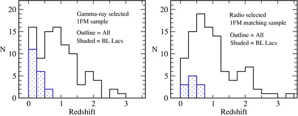
Figure 2. Left panel: redshift distribution of the γ-ray-selected 1FM sample. The full sample is represented by the solid line, and the BL Lac objects are shaded. There is one radio galaxy (J0319+4130 = 3C 84) at z = 0.0176. Right panel: redshift distribution for the radio-selected 1FM matching sample. There are four radio galaxies in the sample, all in the first (z < 0.25) bin.
Download figure:
Standard image High-resolution imageWith respect to the redshifts of the quasars in the two samples, the K-S test suggests a marginal statistical difference in their distributions (D = 0.079, probability = 0.96). There are an insufficient number of radio galaxies to perform any statistical tests on them (there are four in the radio-selected sample; one of these is also in the γ-ray-selected sample). The overall redshift distribution of the γ-ray-selected sample has an additional peak at low redshift, due to the presence of at least nine HSP BL Lac objects that are not in the radio-selected sample (eight additional HSP BL Lac objects lack redshift information). These objects also bring the overall fraction of BL Lac objects up to 35% in the γ-ray-selected sample, as compared to only 13% for the radio-selected sample.
Because of the similarities in the properties and redshift distributions of the γ-ray- and radio-selected samples, for the remainder of this paper we will no longer distinguish between them, referring instead to the joint sample of 173 AGNs.
4.2. γ-Ray Loudness and Synchrotron Peak Frequency
A primary goal of our study is to examine the range of γ-ray loudness (Gr) present in the bright blazar population, and its dependence on other AGN jet properties. Since we have obtained data in several complete regions of the γ-ray–radio plane (i.e., γ-ray-bright/radio-faint; γ-ray-faint/radio-bright; γ-ray-bright/radio-bright) we can be assured of sampling the largest possible range of Gr in the brightest northern-sky blazars. Future studies of the γ-ray-weak/radio-weak region will be important for verifying whether the trends we identify here extend to the fainter blazar population.
In Figure 3, we plot γ-ray luminosity against 15 GHz VLBA luminosity. Despite our use of an average γ-ray luminosity over an 11 month period, the linear relationship for the non-censored data has only moderate scatter (0.6 dex). A linear regression fit to the non-censored data yields log Lγ = (0.92 ± 0.05)log LR + 6.4 ± 2. The Gr values, which reflect the perpendicular distance of the data points from the dashed 1:1 line, span nearly 4 orders of magnitude, from below 3 to ∼15, 000. A clear division between the HSP and lower-synchrotron-peaked BL Lac objects is evident, with the former having higher γ-ray loudness ratios.
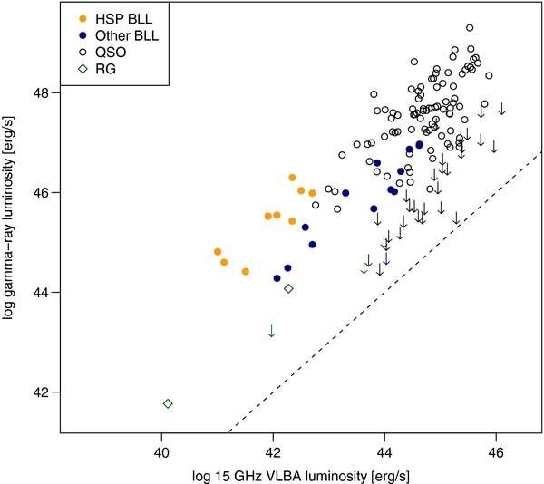
Figure 3. Plot of average γ-ray luminosity vs. median VLBA 15 GHz radio luminosity. The filled circles represent BL Lac objects, with the high-synchrotron peaked ones in orange and others in blue. The open circles represent quasars and the green diamonds radio galaxies. The arrows represent upper limits based on the 11 month LAT data. The dashed line represents the 1:1 luminosity ratio line.
Download figure:
Standard image High-resolution imageNone of the radio galaxies are significantly γ-ray-loud, with ratios all below 65. The quasars and BL Lac objects have significantly different Gr distributions (Figure 4), with the former peaking at Gr ≃ 103 and the latter peaking above 103.5. There is a substantial population of quasars with Gr values below 100, while all of the BL Lac objects (with the exception of J0006−0623) have Fermi associations and Gr > 60. The Peto and Peto modification of Gehan's Wilcoxon two-sample test for censored data rejects the null hypothesis that the quasar and BL Lac Gr values come from the same parent population at the 99.99% confidence level.
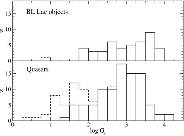
Figure 4. Distribution of γ-ray to radio luminosity ratio for BL Lac objects (top panel) and quasars (bottom panel). Upper limit values for AGNs with no Fermi 1LAC catalog associations are indicated by the dashed lines.
Download figure:
Standard image High-resolution imageThese differences are reflected in Figure 5, which shows γ-ray loudness plotted against the synchrotron SED peak frequency. The BL Lac objects show a roughly linear correlation of the form log Gr = (0.40 ± 0.06)log νs − 2.9 ± 0.9, with a scatter of 0.5 dex, while the quasars show no trend. It is apparent that the BL Lac objects have a higher mean γ-ray loudness value because many of them have synchrotron peaks above ∼1015 Hz. Since the fixed radio bandpass is always located below the synchrotron peak, if we compare two BL Lac objects with identical SED shapes but different synchrotron peak locations, the HSP BL Lac object will have a lower radio flux density, and thus a higher γ-ray loudness value. Figure 6 shows this broad trend for the BL Lac objects, with the HSP jets having generally lower radio flux densities than the LSPs.
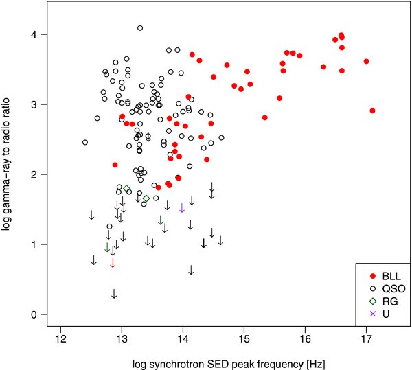
Figure 5. γ-ray to radio luminosity ratio Gr vs. synchrotron SED peak frequency. The red filled circles represent BL Lac objects, the open circles quasars, the green diamonds radio galaxies, and the purple crosses optically unidentified objects. The arrows denote upper limits. The BL Lac objects show a linear trend of increasing γ-ray loudness with SED peak frequency, while no trend exists for the quasars.
Download figure:
Standard image High-resolution image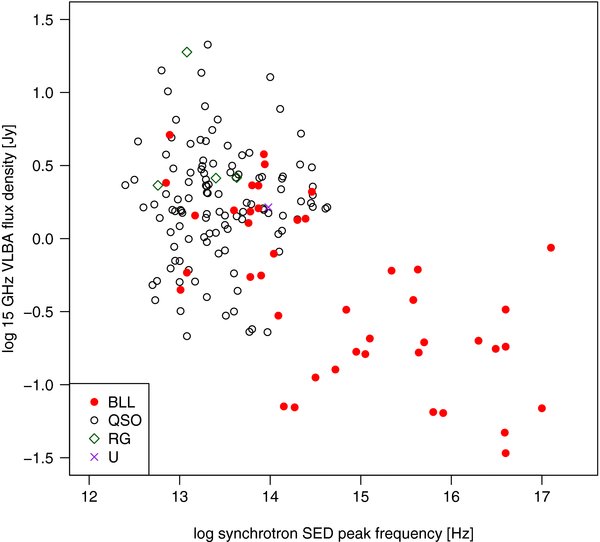
Figure 6. 15 GHz VLBA flux density vs. synchrotron SED peak frequency. The red filled circles represent BL Lac objects, the open circles quasars, the green diamonds radio galaxies, and the purple crosses optically unidentified objects.
Download figure:
Standard image High-resolution imageA similar spectral index effect also occurs as the high-energy SED peak moves in tandem through the Fermi LAT band as the synchrotron peak frequency increases. This is manifested in the strong correlation seen between the γ-ray photon spectral index αG and synchrotron peak frequency for the 1FGL blazars, as described by Abdo et al. (2010d). In Figure 7, we plot γ-ray loudness against photon spectral index. Again we see a good (even tighter) linear correlation for the BL Lac objects and no trend for the quasars. A regression fit to the BL Lac objects, omitting the outlier source J0825+0309, gives log Gr = (− 2.3 ± 0.2)αG + 7.8 ± 0.5, with a scatter of 0.3 dex.
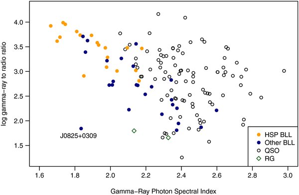
Figure 7. Plot of γ-ray to radio luminosity ratio Gr vs. γ-ray photon spectral index. The filled circles represent BL Lac objects, with the high-synchrotron peaked ones in orange and others in blue. The open circles represent quasars, and the green diamonds radio galaxies. The BL Lac objects show a log-linear trend of decreasing γ-ray loudness with photon spectral index, while no trend exists for quasars.
Download figure:
Standard image High-resolution imageThe continuous trend from LSP to HSP BL Lac objects in Figures 5 and 7 is noteworthy, since it implies a relatively narrow intrinsic range of variation in the SED shapes of the brightest BL Lac objects. Broadly speaking, there are three aspects of an SED that can affect its measured γ-ray loudness parameter. These are the relative positions of the synchrotron and high energy peaks with respect to the fixed γ-ray and radio bands, their relative luminosities (often referred to as the Compton dominance), and the width and shape of each peak. If we take the simplest case of both peaks having equal luminosity and identical parabolic forms in νFν–ν space, then we would expect to have

where νγ and νr are the frequencies of the LAT γ-ray and VLBA radio bands, νh and νs are the frequencies of the high energy and synchrotron peaks, and C1 and C2 are parameters that determine their respective widths.
If both SED peaks have identical parabolic shape (C1 = C2) and the entire SED is then shifted to a higher frequency, such that the peak separation log νh − log νs = C3 remains constant, then we would expect to find a linear relation of the form log Gr = alog νs, with slope

From compilations of observed blazar SEDs (e.g., Abdo et al. 2010e; Chang 2010) we know that in actuality, SED peak shapes are only approximately parabolic, and that there exists a range of C parameter values among the population. These factors would tend to distort any trend between log νs and log Gr from the simple linear one described here. Furthermore, an intrinsic range of Compton dominance parameters would likely destroy any linear relation completely. The fact that we see a scatter of only 0.5 dex for the BL Lac objects therefore implies that the SEDs of the brightest AGNs of this class must have relatively similar shapes, at least much more so than the quasars, which show no νs–Gr correlation. Our results are corroborated by a recent study of the 1LAC by Gupta et al. (2011), who defined a “Compton efficiency” parameter as the ratio of the high-energy (inverse Compton) SED peak luminosity to 8 GHz radio VLA core luminosity. They found a similar trend of higher Compton efficiency with increasing synchrotron peak frequency for BL Lac objects, but no trend for FSRQs.
So far in this discussion we have omitted the possible effects of relativistic beaming on the SED. For the simple case of the same Doppler factor in both the radio- and γ-ray-emitting regions, the entire SED should be blueshifted by the Doppler factor, and the apparent luminosity of both peaks will be increased by Doppler boosting. Models that attribute the high energy peak to inverse Compton scattering of external seed photons by relativistic electrons in the jet predict a higher Doppler boost in γ-rays, because of the additional Lorentz transformation between the seed photon and jet rest frames (Dermer 1995). In this case, when considering a jet at a smaller viewing angle, the resulting increase in Doppler factor boosts the luminosity of the high energy peak to a level much higher than the synchrotron peak, thereby increasing the observed Compton dominance and γ-ray loudness. If the seed photons are internal to the jet, for a single-zone synchrotron self-Compton (SSC) model relatively equal boosting is expected in both regimes; thus, Gr in this case is much less sensitive to Doppler boosting. The fairly good linear Gr–νs correlation for the BL Lac objects therefore favors the SSC process as the dominant emission mechanism in this class of blazars. This is in general agreement with the conclusions of recent studies which have modeled the SEDs of Fermi-detected blazars with detailed synchrotron and inverse-Compton emission models (Abdo et al. 2010e). It should be possible to investigate this issue in much greater depth when more detailed information on the SED parameters of our full sample can be obtained.
4.3. Parsec-scale Radio Jet Properties
4.3.1. Core Brightness Temperature
Nearly all of the AGNs in our sample have a parsec-scale radio jet morphology that is dominated by a bright, flat-spectrum core, which is often unresolved or barely resolved in our mas-scale VLBA images. At our observing frequency of 15 GHz, this core typically represents the region where the jet becomes optically thick, with the true jet nozzle being located upstream (Sokolovsky et al. 2011). The brightness temperature of the core component in our VLBA images measures the compactness of the radio jet emission, and has been previously shown to be correlated with indicators of relativistic beaming, such as superluminal apparent speed (Homan et al. 2006) and radio flux density variability (Tingay et al. 2001; Hovatta et al. 2009).
In Figure 8, we plot core brightness temperature against synchrotron SED peak frequency. The main visible trend is that the HSP BL Lac radio cores tend to be less compact than those of the other AGNs in the sample. We discuss the possible ramifications of this trend on beaming and jet velocity stratification models for HSP BL Lac objects in Section 4.4.
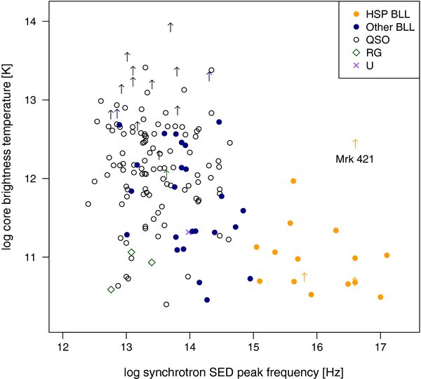
Figure 8. Radio core brightness temperature at 15 GHz vs. synchrotron SED peak frequency. The filled circles represent BL Lac objects, with the high-synchrotron peaked ones in orange and others in blue. The open circles represent quasars, the green diamonds radio galaxies, and the purple crosses optically unidentified objects. The arrows denote lower limits. The radio cores of the high-synchrotron SED peak BL Lac objects tend to be less compact than the other AGNs in our sample. J1104+3812 (Mrk 421) is the only high-synchrotron peaked blazar in the sample with a high core brightness temperature. Not plotted is the unusually low-brightness temperature quasar J0957+5522 (4C +55.17) at νs = 1013.77 Hz, Tb = 108.46 K.
Download figure:
Standard image High-resolution image4.3.2. Apparent Jet Opening Angles
In a previous study of the MOJAVE sample using the initial three months of Fermi data, Pushkarev et al. (2009) found a tendency for the γ-ray-detected blazars to have wider apparent opening angles than the non-detected ones. Since the calculated intrinsic opening angles of the two groups were similar, they concluded that the γ-ray-detected jets were viewed more closely to the line of sight.
We have analyzed the apparent jet opening angles of our sample, and find that they range from 5° to 68°, with a mean of 24°. There is an extended tail to the distribution, with 19 jets having opening angles greater than 40°. With the exception of the quasar J0654+4514, none of the high opening angle jets are highly variable (radio modulation indices all less than 0.26). We find no statistically discernible differences in the opening angle distributions of the different optical or SED classes. We do find a correlation between γ-ray loudness and apparent opening angle, however the relationship is nonlinear (Figure 9). All of the AGNs in the high-opening angle tail (>40°) of the distribution are significantly γ-ray-loud (Gr > 100). The apparent opening angle of a jet is related to the viewing angle and intrinsic opening angle, with smaller intrinsic angles expected for high Lorentz factor jets based on hydrodynamical considerations (Jorstad et al. 2005). The high opening angle jets in our sample are a mixture of BL Lac objects and FSRQ, with a range of synchrotron SED peak frequencies. With jet kinematic information on the sample from the MOJAVE program it will be possible to investigate whether these particular jets are viewed unusually close to the line of sight or have atypically large intrinsic opening angles.
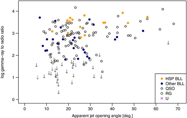
Figure 9. γ-ray to radio luminosity ratio vs. apparent jet opening angle. The filled circles represent BL Lac objects, with the high-synchrotron peaked ones in orange and others in blue. The open circles represent quasars, the green diamonds radio galaxies, and the purple crosses optically unidentified objects. The AGNs with wide apparent opening angles tend to have high γ-ray loudness values.
Download figure:
Standard image High-resolution image4.3.3. Radio Core Polarization Vectors
We compared the direction of the linear polarization vector at the radio core position to the mean jet position angle for our sources, as described in Section 3.2. In some sources such as PKS 1502+106 (Abdo et al. 2010b) and PMN J0948+0022 (Foschini et al. 2011), changes in the core polarization angle have been seen to occur in conjunction with γ-ray flaring events, suggesting a close connection between the radio and γ-ray emission regions. We do not find any correlations between the core polarization vector offset and any γ-ray or SED properties for our sample. However, since the linear polarization vector angles tend to be highly variable in blazars (Jorstad et al. 2005), a more detailed analysis would require truly simultaneous VLBA–Fermi measurements rather than the average γ-ray data that we use in our current study. Another possible reason for the lack of correlations is Faraday effects in the cores, which can rotate the observed polarization vectors. We are currently completing a VLBA rotation measure analysis of the original MOJAVE radio-selected sample (Hovatta et al. 2011) to further investigate this effect.
4.3.4. Radio Core Polarization Level
In Figure 10, we plot the linear fractional polarization level of the VLBA core at the reference epoch versus SED peak frequency. In general the cores of the jets are weakly polarized (<4 %), with increasing fractional polarization levels seen downstream (Lister & Homan 2005). There are no appreciable differences in the BL Lac and FSRQ core polarization distributions, however, as we discuss in Section 4.4, the HSP BL Lac objects tend to have low core polarization levels. We find no trend between 15 GHz radio core polarization and γ-ray loudness, although in the VIPS 5 GHz VLBA survey (Linford et al. 2011) detected core polarization more frequently in LAT-detected AGNs than in the non-LAT ones. We note that the core polarizations tend to vary over time in these jets, which can complicate such analyses. Indeed, in a preliminary investigation of the original MOJAVE radio flux-limited sample, we found that the LAT-detected AGNs tended to have higher median fractional core polarization levels during the first three months of the Fermi mission, as compared to their historical average level (Hovatta et al. 2010). A more complete polarization analysis of our full multi-epoch MOJAVE VLBA data set will be presented in a forthcoming study.
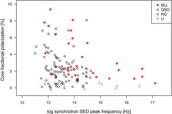
Figure 10. Linear fractional polarization level of VLBA radio core at 15 GHz vs. synchrotron SED peak frequency. The red filled circles represent BL Lac objects, the open circles quasars, the green diamonds radio galaxies, and the purple crosses optically unidentified objects. The arrows denote upper limits.
Download figure:
Standard image High-resolution image4.3.5. Radio Variability
The hallmark flux variability seen in blazars is believed to be closely related to Doppler beaming (Aller et al. 1992; Lähteenmäki et al. 1999; Hovatta et al. 2009) since it can significantly heighten the magnitudes of flaring events and shorten their apparent timescales (e.g., Lister 2001b). AGN jets have also been found to be in a more active radio state within several months from LAT detection of their strong γ-ray emission (Kovalev et al. 2009; Pushkarev et al. 2010). The AGNs in our sample are indeed highly variable, with 51 of 144 sources having standard deviations greater than 15% of their mean flux density level over an 11 month period. In their full sample of over 1000 sources, Richards et al. (2011) found the FSRQs to have significantly higher variability amplitudes than the BL Lac objects. We do not see this distinction in our sample, however, most likely because ours contain a smaller proportion of HSP BL Lac objects. The latter tend to have moderately low radio modulation indexes, as seen in Figure 11.
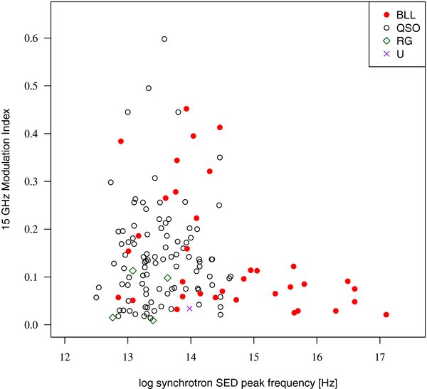
Figure 11. Radio modulation index at 15 GHz vs. synchrotron SED peak frequency. The filled circles represent BL Lac objects, the open circles quasars, the plus symbols radio galaxies, and the crosses optically unidentified objects. None of the blazars with synchrotron SED peaks above 1015 Hz show high-amplitude radio variability.
Download figure:
Standard image High-resolution image4.4. High-synchrotron-peaked AGN Jets and the BL Lac Blazar Class
Previous studies of the full 1LAC catalog by the LAT team (Abdo et al. 2010d, 2010e) have established that HSP BL Lac objects have fundamentally different γ-ray properties than the γ-ray-loud FSRQs. In our study, we have found that the HSP BL Lac objects are characterized by high γ-ray to radio luminosity ratios and lower than average radio core compactness. Given these differences seen in both the radio and γ-ray regimes, a fundamental question remains as to whether the lower synchrotron-peaked BL Lac objects also form a jet population distinct from the FSRQs. The continuity of the trend between SED peak frequency and γ-ray loudness (Figure 5) would suggest that their SED shapes are similar to the HSP BL Lac objects, and thus they should be unified with them. They are also more similar to the HSPs in terms of their radio luminosity, as compared to the generally more luminous FSRQs (Figure 3).
If we directly compare the radio properties of the LSP BL Lac objects and LSP FRSQs in our sample, we find that the LSP BL Lac objects have higher mean fractional linear polarization (4.8 ± 2.8 versus 2.5 ± 1.7; t = 3.02, p = 0.992 according to a Welch Two Sample t-test), although both classes span roughly the same range of extreme values (Figure 10). It is possible that beam depolarization effects may lower the mean value for the FSRQs, since they are typically at higher redshift than the BL Lac objects and are thus imaged with poorer spatial resolution.
However, if we compare the LSP and HSP BL Lac objects, which have similar redshift ranges, we find that the latter have consistently low core polarization and modulation indices, as well as lower than average radio core brightness temperatures. Since high radio variability, core polarization, and brightness temperature are generally associated with high Doppler boosted jets (e.g., Lister 2001a; Tingay et al. 2001; Hovatta et al. 2009), the trends we find in our sample support the following scenario for the brightest γ-ray and radio blazars in the sky. Because of their higher intrinsic γ-ray loudness ratios and low redshifts, the HSP BL Lac objects do not need to be as highly beamed to enter into flux-limited γ-ray and radio samples, thus they tend to have lower Doppler boosting factors than other blazar classes. The LSP BL Lac objects are less intrinsically luminous than the FSRQs, but their moderately high-intrinsic γ-ray loudness ratios and Doppler boosting factors combine to give them apparent γ-ray and radio luminosities comparable to the fainter end of the FSRQ distribution.
The above scenario is supported by the previous results of Nieppola et al. (2008), who found a general trend of decreasing Doppler factor with increasing synchrotron SED peak frequency. Their sample only included blazars of the LSP and ISP classes, however. A potential test can be made with parsec-scale superluminal motion measurements, which set an upper limit on the viewing angle and a lower limit on the bulk jet Lorentz factor (see, e.g., Urry & Padovani 1995). One of the main unresolved problems for HSP BL Lacs has been the relatively slow apparent jet speeds detected for these objects (Piner & Edwards 2004; Piner et al. 2010), despite the need for large Doppler factors to account for rapid variability seen in γ-rays and to accurately model their SEDs (see, e.g., Henri & Saugé 2006). Several models have been put forward to address this “Doppler factor crisis,” including decelerating flows (Georganopoulos & Kazanas 2003), and stratified spine–sheath models (Celotti et al. 2001; Tavecchio & Ghisellini 2008), in which the γ-rays originate in a high-velocity jet spine, while the radio emission (and moving blobs) are associated with a lower-Lorentz factor sheath. In this manner the radio and γ-ray emission can have independent Doppler factors. As we discussed in Section 3.3, however, uncorrelated beaming factors for the synchrotron and high-energy peaks would likely destroy any linear relation between SED synchrotron peak and γ-ray loudness, in contrast to what we see for the BL Lac objects in our survey (Figure 5). A more recent model put forward by Lyutikov & Lister (2010) involving non-steady magnetized outflows suggests the existence of different, yet correlated, Doppler factors for the two SED peak regions, which can potentially preserve the Gr versus synchrotron SED peak relation. With the MOJAVE program we are currently obtaining multi-epoch VLBA measurements of all the γ-ray-selected radio jets in our sample, which will allow us to investigate further the connections between synchrotron SED peak frequency, apparent jet speed, jet opening angle, and Doppler factor in the brightest blazars.
5. SUMMARY
We have obtained single-epoch 15 GHz MOJAVE program VLBA images68 of two complete flux-limited samples of blazars north of declination −30° and >10° from the Galactic plane. The first sample consists of the brightest sources associated with AGNs that were detected by the Fermi LAT instrument during its first 11 months of operations. The second sample contains all radio-loud AGNs known to have exceeded a 15 GHz VLBA flux density of 1.5 Jy during the same time period. There are 116 AGNs in the γ-ray-selected sample and 105 AGNs in the matching radio one, with 48 AGNs in common to both samples. By covering two complete regions of the γ-ray–radio-flux plane, we are able to sample the widest possible range of γ-ray loudness in bright blazars. Our results can be compared with those of Linford et al. (2011), who studied a larger, radio flux-limited sample of fainter AGNs with 5 GHz VLBA data obtained several years before the launch of Fermi. We summarize our major findings as follows.
- 1.There is a 28% overlap in our samples of the brightest γ-ray- and radio-selected AGNs in the northern sky. We find no major differences in the sample redshift distributions, with the exception of a small number of HSP BL Lac objects which appear only in the γ-ray-selected sample. At the highest flux levels therefore, γ-ray- and radio-selected blazars are essentially selected from the same general parent population.
- 2.We have tabulated a γ-ray loudness parameter (Gr) for all of the sources in our sample, including upper limits for the non-LAT associated sources in our radio-selected sample. The non-censored Gr values span nearly 4 orders of magnitude, reflecting the wide range of SED parameters in the bright blazar population. However, within the BL Lac optical class, we find a linear relation (scatter = 0.5 dex) between synchrotron SED peak frequency νs and Gr, with the HSP BL Lac objects being more γ-ray-loud. Such a linear relationship is expected if the overall range of SED shape is relatively narrow within the BL Lac population, as the radio flux density will drop and γ-ray flux will increase as the SED is successively shifted to higher frequencies, thereby increasing the γ-ray loudness. A further consequence of the observed correlation is that the amount of Doppler boosting must be correlated in the radio and γ-ray emission regimes of BL Lac jets. The external seed-photon inverse-Compton model is not favored for the γ-ray emission of the BL Lac objects in our sample, since it predicts higher boosting of the γ-rays with respect to the radio. Any range of Doppler factor within the BL Lac population would therefore destroy any expected linear correlation between Gr and νs in the external Compton scenario.
- 3.In terms of their 15 GHz radio properties, the HSP BL Lac objects in our sample are distinguished by their lower than average radio core brightness temperatures. None of them display large radio modulation indices or high linear core polarization levels. Given the known association of such properties with relativistic beaming, we suggest that the HSP BL Lac objects have generally lower Doppler factors than the lower-synchrotron peaked BL Lac objects or FSRQs in our sample. They are able to meet our flux-selection criteria primarily because of their high intrinsic γ-ray ratios and low redshifts. The continuity of the observed Gr–νs relation suggests that the high- and low-synchrotron peaked BL Lac objects are part of the same parent population. The latter have moderate intrinsic γ-ray loudness ratios and Doppler boosting factors which combine to give them apparent γ-ray and radio luminosities that are comparable to the fainter end of the FSRQ distribution.
- 4.We confirm the results of a previous analysis by Pushkarev et al. (2009), who found that Fermi-associated AGNs tend to have wider apparent jet opening angles. Using a larger (11 month versus 3 month) Fermi data set on our more comprehensive blazar sample, we find that all of the highest opening angle jets (>40°) in our sample are significantly γ-ray loud.
The MOJAVE program is continuing to investigate these issues by obtaining multi-epoch VLBA measurements of all the γ-ray-selected radio jets in our sample. Together with more complete SED information, light curves, and deep EVLA images we aim to gain a fuller understanding of the connections between synchrotron SED peak frequency, Compton dominance, apparent jet speed, and Doppler factor in the brightest blazars.
We thank M. H. Cohen and D. C. Homan for helpful comments on the manuscript.
C. S. Chang was a former member of the International Max Planck Research School for Astronomy and Astrophysics. C. S. Chang acknowledges support by the EU Framework 6 Marie Curie Early Stage Training programme under contract number MEST-CT-2005-19669 “Estrela.”
Y. Y. Kovalev was supported in part by the return fellowship of the Alexander von Humboldt Foundation and the Russian Foundation for Basic Research (RFBR) grants 08-02-00545 and 11-02-00368.
E. Ros acknowledges partial support by the Spanish MICINN through grant AYA2009-13036-C02-02.
Work at UMRAO was made possible by grants from the NSF and NASA and by support from the University of Michigan.
The Fermi LAT Collaboration acknowledges generous ongoing support from a number of agencies and institutes that have supported both the development and the operation of the LAT as well as scientific data analysis. These include the National Aeronautics and Space Administration and the Department of Energy in the United States, the Commissariat à l'Energie Atomique and the Centre National de la Recherche Scientifique/Institut National de Physique Nucléaire et de Physique des Particules in France, the Agenzia Spaziale Italiana and the Istituto Nazionale di Fisica Nucleare in Italy, the Ministry of Education, Culture, Sports, Science and Technology (MEXT), High Energy Accelerator Research Organization (KEK) and Japan Aerospace Exploration Agency (JAXA) in Japan, and the K. A. Wallenberg Foundation, the Swedish Research Council and the Swedish National Space Board in Sweden.
Additional support for science analysis during the operations phase is gratefully acknowledged from the Istituto Nazionale di Astrofisica in Italy and the Centre National d'Études Spatiales in France.
The MOJAVE project is supported under National Science Foundation grant AST-0807860 and NASA Fermi grant NNX08AV67G.
This research has made use of the NASA/IPAC Extragalactic Database (NED) which is operated by the Jet Propulsion Laboratory, California Institute of Technology, under contract with the National Aeronautics and Space Administration.
This work made use of the Swinburne University of Technology software correlator (Deller et al. 2011), developed as part of the Australian Major National Research Facilities Programme and operated under licence.
The National Radio Astronomy Observatory is a facility of the National Science Foundation operated under cooperative agreement by Associated Universities, Inc.
The VLBA is a facility of the National Science Foundation operated by the National Radio Astronomy Observatory under cooperative agreement with Associated Universities, Inc.
Facilities: VLBA - Very Long Baseline Array, Fermi(LAT) - Fermi Gamma-Ray Space Telescope (formerly GLAST), UMRAO - University of Michigan Radio Astronomy Observatory 26m telescope at Peach Mountain, OVRO:40m - Owens Valley Radio Observatory's 40 meter Telescope
APPENDIX: REDSHIFT INFORMATION
We summarize the current status of those blazars in our sample which either do not have a spectroscopic redshift listed in Table 1 or have uncertain or conflicting reported redshift values in the literature.
J0050−0929. The NED value of z = 0.634 from Rector & Stocke (2001) is based on a very weak emission line and is listed by those authors as tentative. This line was not seen by Shaw et al. (2009) or Sbarufatti et al. (2006) in their optical spectra. Based on the absence of host galaxy absorption features in the optical spectrum Shaw et al. (2009) find z > 0.44, and Sbarufatti et al. (2006) find z > 0.3. Meisner & Romani (2010) obtain z > 0.27 based on the measured optical host galaxy magnitude.
J0112+2244. Healey et al. (2008) list z = 0.265 based on an unpublished spectrum. Shaw et al. (2009) find z > 0.24 and Sbarufatti et al. (2009) get z > 0.25 based on the absence of host galaxy absorption features in the optical spectrum.
J0120−2701. The NED value of z = 0.559 is a lower limit from Stickel et al. (1993a).
J0136+3908. We could not find any published redshift value for this source.
J0237+2848. The NED value of z = 1.213 attributed to Schmidt (1977) is different from the z = 1.207 that is reported in that reference.
J0222+4302 = 3C 66A. As discussed by Finke et al. (2008) and Bramel et al. (2005), the NED redshift value of z = 0.444 is highly unreliable. Finke et al. (2008) obtained z > 0.096 based on their optical spectrum.
J0316+0904. We could not find any published redshift value for this source.
J0433+2905. Meisner & Romani (2010) obtain z > 0.48 based on the measured optical host galaxy magnitude. The origin of the z = 0.97 value listed in BZCAT (Massaro et al. 2009) is unknown.
J0509+0541. Meisner & Romani (2010) obtain z > 0.38 based on the measured optical host galaxy magnitude.
J0608−1520. M. S. Shaw et al. (2011, in preparation) have obtained an optical spectrum of this source and find emission lines indicating a quasar at z = 1.094.
J0612+4122. Meisner & Romani (2010) obtain z > 0.69 based on the measured optical host galaxy magnitude.
J0630−2406. Landt & Bignall (2008) list z = 1.238, which is a lower limit based on Mg ii absorption lines in their unpublished optical spectrum.
J0654+5042. M. S. Shaw et al. (2011, in preparation) have obtained an optical spectrum of this source and find emission lines indicating a quasar at z = 1.253.
J0738+1742. The NED value of z = 0.424 is a lower limit determined by Rector & Stocke (2001) on the basis of absorption systems in the optical spectrum.
J0818+4222. Britzen et al. (2008) list z = 0.245 based on an unpublished spectrum. The NED value of z = 0.53 is attributed to Sowards-Emmerd et al. (2005) but does not appear in that paper. An optical spectrum obtained by M. S. Shaw et al. (2011, in preparation) shows no visible features. Sbarufatti et al. (2005) found z > 0.75 based on a lower limit to the host galaxy magnitude.
J1037+5711. Véron-Cetty & Véron (2000) classify this source as a BL Lac object. We were unable to find any redshift value in the literature.
J1248+5820. The SDSS optical spectrum (Abazajian et al. 2005) yields no reliable redshift, and an unpublished spectrum by M. S. Shaw et al. (2011, in preparation) shows no spectral features.
J1215−1731. We were not able to find any published redshift value for this optically unidentified source, which lies extremely close on the sky to a bright star.
J1221+2813 = W Comae. The NED redshift value of z = 0.102 is likely incorrect, as discussed by Finke et al. (2008). The latter authors constrain the redshift to z > 0.104 using their optical spectrum.
J1303+2433. Glikman et al. (2007) list z = 0.993 but give no reference for the origin of this redshift. An optical spectrum obtained by M. S. Shaw et al. (2011, in preparation) yields z > 0.769.
J1427+2348. Shaw et al. (2009) find z > 0.03, while Meisner & Romani (2010) get z > 0.23 based on host galaxy magnitude.
J1516+1932. The NED redshift value of z = 1.07 from Persic & Salucci (1986) is based on tentative identifications of very faint emission lines in the optical spectrum of Wilkes et al. (1983) and has not been subsequently confirmed. An optical spectrum obtained by M. S. Shaw et al. (2011, in preparation) shows no spectral features.
J1532+6129. Shaw et al. (2009) find z > 0.63 based on the absence of host galaxy absorption features in the optical spectrum, while Meisner & Romani (2010) obtain z > 0.39 based on the measured optical host galaxy magnitude.
J1555+1111. The z = 0.360 redshift value from Miller & Green (1983) was shown by Falomo & Treves (1990) and Falomo et al. (1994) to be incorrect. Based on the absence of host galaxy absorption features in the optical spectrum, Sbarufatti et al. (2006) find z > 0.09. Danforth et al. (2010) analyze the Lyman absorber properties of the far-UV spectrum of this source and find 0.395 < z < 0.58.
J1719+1745. Sowards-Emmerd et al. (2005) list z = 0.137 based on an unpublished optical spectrum. Shaw et al. (2009) obtain z > 0.58 based on the measured optical host galaxy magnitude.
J1725+1152. As described by Sbarufatti et al. (2006), the tentative NED redshift of z = 0.018 from Griffiths et al. (1989) has not been confirmed in several subsequent spectroscopic observations. Based on the absence of host galaxy absorption features in the optical spectrum, Sbarufatti et al. (2006) find z > 0.17.
J1903+5540. Meisner & Romani (2010) obtain z > 0.58 based on the measured optical host galaxy magnitude.
J2236−1433. Sbarufatti et al. (2006) trace the oft-cited erroneous NED redshift of z = 0.325 to a clerical error. Based on the absence of host galaxy absorption features in the optical spectrum, they find z > 0.65. An unpublished optical spectrum by M. S. Shaw et al. (2011, in preparation) shows no spectral features.
J2243+2021. Meisner & Romani (2010) obtain z > 0.39 based on the measured optical host galaxy magnitude.
Footnotes
- 67
- 68
MOJAVE data archive: http://www.physics.purdue.edu/MOJAVE