ABSTRACT
We present time-resolved and phase-resolved variability studies of an extensive X-ray high-resolution spectral data set of the δ Ori Aa binary system. The four observations, obtained with Chandra ACIS HETGS, have a total exposure time of  ks and provide nearly complete binary phase coverage. Variability of the total X-ray flux in the range of 5–25 Å is confirmed, with a maximum amplitude of about ±15% within a single
  ks observation. Periods of 4.76 and 2.04 days are found in the total X-ray flux, as well as an apparent overall increase in the flux level throughout the nine-day observational campaign. Using 40 ks contiguous spectra derived from the original observations, we investigate the variability of emission line parameters and ratios. Several emission lines are shown to be variable, including S xv, Si xiii, and Ne ix. For the first time, variations of the X-ray emission line widths as a function of the binary phase are found in a binary system, with the smallest widths at ϕ = 0.0 when the secondary δ Ori Aa2 is at the inferior conjunction. Using 3D hydrodynamic modeling of the interacting winds, we relate the emission line width variability to the presence of a wind cavity created by a wind–wind collision, which is effectively void of embedded wind shocks and is carved out of the X-ray-producing primary wind, thus producing phase-locked X-ray variability.
1. INTRODUCTION
Stellar winds of hot massive stars, primarily those with M ≥ 8 M⊙, have important effects on stellar and galactic evolution. These winds provide enrichment to the local interstellar medium via stellar mass loss. On a larger scale, the cumulative enrichment and energy from the collective winds of massive stars in a galaxy are expected to play a pivotal role in driving galactic winds (Leitherer et al. 1992; Oppenheimer & Davé 2006; McKee & Ostriker 2007). The number of massive stars in any star-forming galaxy, as well as their tendency to be found in clusters, are critical parameters for determining a galaxy’s energy budget and evolution. Oskinova (2005) and Agertz et al. (2013) showed that the energy from the winds of massive stars will dominate over the energy from supernovae in the early years of massive star cluster evolution. While substantial progress has been made over the last several decades in modeling massive star winds (Puls et al. 1996), many questions remain, such as the degree of clumping of the winds, the radial location of different ions and temperature regimes in the wind with respect to the stellar surface, and the origin of Corotating Interaction Regions (CIRs) representing large-scale wind perturbations. X-ray observations have provided powerful diagnostic tools for testing models, but a fully consistent description of the detailed structure of a stellar wind is still elusive.
Variability in the winds of massive stars can be an important probe of the structure of the stellar winds. There can be multiple causes of X-ray variability in massive stars. Large-scale structures in the winds, as traced by Discrete Absorption Components (DACs; Kaper et al. 1999) and possibly linked to CIRs, may be associated with shocks in the wind and thereby potentially affect the X-ray emission. X-ray variations of this type have probably been detected for ζ Oph, ζ Pup, and ξ Per (Oskinova et al. 2001; Nazé et al. 2013; Massa et al. 2014). Also, X-ray variability with the same period as, but larger amplitude than, known pulsational activity in the visible domain was recently detected in  CMa (Oskinova et al. 2014) and possibly in the hard band of β Cru (Cohen et al. 2008). The exact mechanism giving rise to these changes remains unclear. Notably, other pulsating massive stars do not show such X-ray “pulsations,” such as β Cen (Raassen et al. 2005) and β Cep (Favata et al. 2009). Smaller-scale structures, such as clumps, can also produce X-rays, albeit at lower energies than large-scale structures. It is also possible that some X-ray variations in massive stars are stochastic in nature and are not correlated with any currently known timescale.
Another cause for X-ray variability is possible in magnetic stars. When a strong global magnetic field exists, the stellar wind is forced to follow the field lines, and the wind flowing from the two stellar hemispheres may then collide at the equator, generating X-rays (Babel & Montmerle 1997). Such recurrent variations have been detected in  Ori C (Gagné et al. 2005; Stelzer et al. 2005), HD 191612 (Nazé et al. 2010), and possibly Tr16-22 (Nazé et al. 2014), though the absence of large variations in the X-ray emission of the magnetic star τ Sco is puzzling in this context (Ignace et al. 2010). Even stronger, but very localized, magnetic fields could also be present, e.g., associated with bright spots on the stellar surface that are required to create CIRs (Cranmer & Owocki 1996; Cantiello et al. 2009).
In multiple systems, the collision of the wind of one star with the wind of another can produce X-ray variations (Stevens et al. 1992). Wind–wind collision emission may vary with binary phase, with inverse distance in eccentric systems, or due to changes in line of sight absorption, as observed in HD 93403 (Rauw et al. 2002), Cyg OB2 9 (Nazé et al. 2012), V444 Cyg (Lomax et al. 2015), and possibly HD 93205 (Antokhin et al. 2003).
Delta Ori A (Mintaka, HD 36486, 34 Ori) is a nearby multiple system that includes the close eclipsing binary, δ Ori Aa1 (O9.5 II: Walborn 1972) and δ Ori Aa2 (B1 V: Shenar et al. 2015, herein Paper IV), with a period of ≈5.73 days (Harvin et al. 2002; Mayer et al. 2010). This close binary is orbited by a more distant companion star, δ Ori Ab (≈B0 IV: Pablo et al. 2015, herein Paper III; Paper IV), with a period of  years (Heintz 1987; Perryman & ESA 1997; Tokovinin 2014). The components Aa1 and Aa2 are separated by about 43
  (2.6 RAa1; Paper III), and the inclination of ≈76° ± 4° (Paper III) ensures eclipses. We acquired
  ks of high resolution X-ray grating spectra with a Chandra Large Program to observe a nearly full period of δ Ori Aa (Corcoran et al. 2015, herein Paper I). Simultaneous with the acquisition of the Chandra data, Microvariability and Oscillations of Stars (MOST) space-based photometry and ground-based spectroscopy at numerous geographical locations were obtained and are reported in Paper III. Table 2 lists the spectral types and radii of the Idel Ori Aa1 and Aa2, as well as the orbital parameters and the MOST secondary periods.
Previous X-ray observations of the δ Ori A system from Einstein showed no significant variability (Grady et al. 1984). ROSAT data for δ Ori A were studied by Haberl & White (1993), who found modest 2σ variability but no obvious phase dependence; the Corcoran (1996) reanalysis of the ROSAT data showed similar results. A single previous Chandra HETGS observation of δ Ori Aa was analyzed by Miller et al. (2002). Fitting the emission lines using Gaussian profiles, they found the profiles to be symmetrical and of low FWHM, considering the estimated wind velocity. The 60 ks exposure time covers about 12% of the orbital period. Raassen & Pollock (2013) analyzed a Chandra LETGS observation with an exposure time of 96 ks, finding some variability in the zeroth order image; they were not able to detect any variability in the emission lines between two time splits of the observation.
This paper is part of a series of papers. The other papers in this series address the parameters of the composite Chandra  ks spectrum (Paper I), the simultaneous MOST and spectroscopic observations (Paper III), and UV–optical–X-ray wind modeling (Paper IV). In this paper (Paper II), we investigate variability in the X-ray flux in the Chandra spectra. Section 2 describes the Chandra data and processing techniques. Section 3 discusses the overall X-ray flux variability of the observations and period search. Time-resolved and phase-resolved analyses of emission lines are presented in Section 4. In Section 5, we relate our results of phase-based variable emission line widths to a colliding wind model developed for this binary system in Paper I and discuss possible additional sources of variability in δ Ori Aa. Section 6 presents our conclusions.
2. OBSERVATIONS AND DATA REDUCTION
Delta Ori Aa was observed with the Chandra ACIS instrument using the HETGS (Canizares et al. 2005) for a total exposure time of  ks, covering parts of three binary periods (see Table 2 for a list of observations and binary phases). Four separate observations were obtained within a nine-day interval. The HETGS consists of two sets of gratings: the Medium Energy Grating (MEG) with a range of 2.5–31 Å (0.4–5.0 keV) and resolution of 0.023 Å FWHM, and the High Energy Grating (HEG) with a range of 1.2–15 Å (0.8–10 keV) and resolution of 0.012 Å FWHM. The resolution is approximately independent of wavelength. The Chandra ACIS detectors record both MEG and HEG dispersed grating spectra as well as the zeroth order image. Due to spacecraft power considerations, it was necessary to use only five ACIS CCD chips instead of the requested six for these observations. Chip S5 was not used, meaning wavelengths longer than about 19 Å in the MEG dispersed spectra and about 9.5 Å in the HEG dispersed spectra were only recorded for the “plus” side of the dispersed spectra, reducing the number of counts and effective exposure in these wavelength regions. The standard data products distributed by the Chandra X-ray Observatory were further processed with TGCat software18
(Huenemoerder et al. 2011). Specifically, each level 1 event file was processed into a new level 2 event file using a package of standard CIAO analysis tools (Fruscione et al. 2006). Additionally, appropriate redistribution matrix (RMF) and area auxiliary response (ARF) files were calculated for each order of each spectrum. TGCat processing produced analysis products with supplemental statistical information, such as broad- and narrow-band count rates.
ks, covering parts of three binary periods (see Table 2 for a list of observations and binary phases). Four separate observations were obtained within a nine-day interval. The HETGS consists of two sets of gratings: the Medium Energy Grating (MEG) with a range of 2.5–31 Å (0.4–5.0 keV) and resolution of 0.023 Å FWHM, and the High Energy Grating (HEG) with a range of 1.2–15 Å (0.8–10 keV) and resolution of 0.012 Å FWHM. The resolution is approximately independent of wavelength. The Chandra ACIS detectors record both MEG and HEG dispersed grating spectra as well as the zeroth order image. Due to spacecraft power considerations, it was necessary to use only five ACIS CCD chips instead of the requested six for these observations. Chip S5 was not used, meaning wavelengths longer than about 19 Å in the MEG dispersed spectra and about 9.5 Å in the HEG dispersed spectra were only recorded for the “plus” side of the dispersed spectra, reducing the number of counts and effective exposure in these wavelength regions. The standard data products distributed by the Chandra X-ray Observatory were further processed with TGCat software18
(Huenemoerder et al. 2011). Specifically, each level 1 event file was processed into a new level 2 event file using a package of standard CIAO analysis tools (Fruscione et al. 2006). Additionally, appropriate redistribution matrix (RMF) and area auxiliary response (ARF) files were calculated for each order of each spectrum. TGCat processing produced analysis products with supplemental statistical information, such as broad- and narrow-band count rates.
MOST photometry observations of δ Ori Aa were obtained for approximately three weeks, including the nine days of Chandra observations. Figure 1 shows the simultaneous MOST light curve aligned in time to the Chandra light curve. The Chandra light curve in this figure is the ±1 orders of the HEG and MEG combined in the  Å range, binned at 4 ks, with Poisson errors. Figure 2 shows the same data plotted with binary phase rather than time. The MOST light curves from several orbits are averaged and overplotted in the figure to show the optical variability.
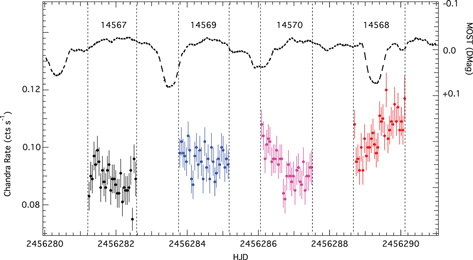
Figure 1. Chandra X-ray light curve from the 2012 campaign with the simultaneous continuous MOST optical light curve. The time intervals for each of the Chandra observations are delineated with vertical lines with the Chandra observation ID (ObsID in Table 2) at the top of the figure. The Chandra light curves were calculated from the dispersed spectra in each observation. The four observations are separated by gaps due to the passage of Chandra through the Earth’s radiation zone as well as necessary spacecraft thermal control, during which time continued δ Ori Aa observations were not possible. Chandra counts per second are on the left y axis. MOST differential magnitudes are on the right y axis.
Download figure:
Standard image High-resolution image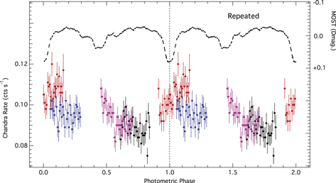
Figure 2. Phased Chandra X-ray light curve from the 2012 campaign with the simultaneous continuous MOST optical light curve. The mean δ Ori Aa MOST optical light curve is plotted above the Chandra X-ray light curve. The four Chandra observations are shown in red, magenta, blue, and black. The binary phase is on the x axis, the MOST differential magnitude is on the right y axis, and the Chandra count rate is on the left y axis. The MOST light curves have been smoothed and both light curves have been repeated for one binary orbit for clarity.
Download figure:
Standard image High-resolution imageIn this paper, ϕ = 0.0 refers to the binary orbital period and denotes the time when the secondary is in front of the primary (deeper optical minimum) and ϕ = 0.5 denotes the time when the primary is approximately in front of the secondary (shallower optical minimum). While primary minimum is a definition, the secondary minimum at ϕ = 0.5 is only approximate, since the orbit is slightly elliptical and also varies slowly with apsidal motion. The actual secondary minimum is currently ϕ = 0.45 (Paper III). Actual current quadrature phases are ϕ = 0.23 and 0.78. To avoid confusion, we use the phases in this paper that would be assumed with a circular orbit (i.e., ϕ = 0 for inferior conjunction, ϕ = 0.5 for superior conjunction, and ϕ = 0.25 and 0.75 for quadrature). Also, we use the ephemeris of Mayer et al. (2010). No evidence of X-ray emission from the tertiary star was seen in any of the Chandra observations (Paper I), so the spectra represent only δ Ori Aa1 and Aa2.
Table 1. System Parameters for δ Ori Aa1+Aa2
| Parameter | Value |
|---|---|
| Sp. Type (Aa1) | O9.5IIa,b,d |
| Sp. Type (Aa2) | B1Va |
| D (pc) | 380 (adopted)a |
 (Aa1) (Aa1) |

|
 (Aa2) (Aa2) |

|
| Binary Periodb | |

|
 d
d
|
| E0 (primary min, HJD) | 2456277.790 ± 0.024 |
| T0 (periastron, HJD) | 2456295.674 ± 0.062 |

|
43.1 ± 1.7 |
| i (deg) | 76.5 ± 0.2 |
| ω (deg) | 141.3 ± 0.2 |
 (deg yr−1) (deg yr−1) |
1.45 ± 0.04 |
| e | 0.1133 ± 0.0003 |
| γ (km s−1) | 15.5 ± 0.7 |
| Periastron-based ϕ | 0.116+Photometric-based ϕ |
| MOST Optical Secondary Periods (days) | |
| MOSTF1 | 2.49 ± 0.332 |
| MOSTF2 | 4.614 ± 1.284 |
| MOSTF3 | 1.085 ± 0.059 |
| MOSTF4 | 6.446 ± 2.817 |
| MOSTF5 | 3.023 ± 0.503 |
| MOSTF6e | 29.221 ± 106.396 |
| MOSTF7 | 3.535 ± 0.707 |
| MOSTF8 | 1.01 ± 0.051 |
| MOSTF9 | 1.775 ± 0.162 |

|
2.138 ± 0.24 |

|
1.611 ± 0.133 |

|
0.809 ± 0.032 |

|
0.748 ± 0.027 |
Note.
aShenar et al. (2015). bfrom the low-mass model solution of Pablo et al. (2015). cSota et al. (2014). dMayer et al. (2010). eThis peak is likely an artifact due to a trend in the data. It is not considered real, but it is formally significant and included in the fit.Download table as: ASCIITypeset image
3. OVERALL VARIABILITY OF X-RAY FLUX
The light curve of the dispersed Chandra spectrum of δ Ori Aa, shown in the lower part of Figure 1, shows that the spectrum was variable throughout in X-ray flux with a maximum amplitude of about ±15% in a single observation. During the first and second observations the X-ray flux varied by ≈5%–10%, followed by a ≈15% decrease in the third and a ≈15% increase in the fourth. Note that none of the X-ray minima in the residual light curve aligns with an optical eclipse of the δ Ori Aa system. Figure 1 suggests an increase in overall X-ray flux with time. From the beginning to end of the nine-day campaign there is a ≈25% increase in the mean count rate. The best linear fit to the entire light curve is 96.04 counts/days + 0.002 counts/days HJD, with equal weights for all points.
We first did a rough period search on the δ Ori Aa Chandra light curves using the software package Period04 (Lenz & Breger 2005), and found peaks around 4.8 and 2.1 days. This method uses a speeded-up Deeming algorithm (Kurtz 1985) that is not appropriate for sparse data sets such as ours because it assumes the independence of sine and cosine terms to be valid only for regular light curves. Therefore, to verify this preliminary conclusion and get final results, we rather rely on several methods specifically suitable to such sparse light curves: the Fourier period search optimally adapted to sparse data sets (Heck et al. 1985; Gosset et al. 2001, see Figure 5), as well as variance and entropy methods (e.g., Schwarzenberg-Czerny 1989; Cincotta et al. 1999). The results of all these methods were consistent within the errors of each other.
Table 2. 2013 Chandra Observations of δ Ori Aa
| ObsID | Start | Start | End | End | Midpoint | Midpoint |

|
Exposure | Roll |
|---|---|---|---|---|---|---|---|---|---|
| HJD | Phase | HJD | Phase | HJD | Phase | days | s | deg | |
| 14567 | 2456281.21 | 396.604 | 2456282.58 | 396.843 | 2456281.90 | 396.724 | 1.37 | 114982 | 345.2 |
| 14569 | 2456283.76 | 397.049 | 2456285.18 | 397.297 | 2456284.47 | 397.173 | 1.42 | 119274 | 343.2 |
| 14570 | 2456286.06 | 397.450 | 2456287.52 | 397.705 | 2456286.79 | 397.578 | 1.46 | 122483 | 83.0 |
| 14568 | 2456288.67 | 397.905 | 2456290.12 | 398.159 | 2456289.39 | 398.032 | 1.45 | 121988 | 332.7 |
Download table as: ASCIITypeset image
Using these tools, we first looked for periods in the raw  lightcurve data. A period of 5.0 ± 0.3 days was found with an amplitude of
  . We then removed the linear trend described above from the raw data, producing a residual light curve. The period searches were repeated, with an identified period of 4.76 ± 0.3 days (amplitude =
  ). After pre-whitening the residual data in Fourier space for this period, an additional significant period of 2.04 ± 0.05 days (amplitude =
  ) was found. Each of these periods has a Significance Level (SL) of
  1% with the definition of SL as a test of the probability of rejecting the null hypothesis given that it is true. If the SL is a very small number, the null hypothesis can be rejected because the observed pattern has a low probability of occurring by chance. Figure 3 shows the results of the Fourier period search method for the raw, residual, and pre-whitened light curves, which produced periods of 5.0, 4.76, and 2.04 days, respectively. Table 3 lists the frequency, period, and amplitude of the periods. Figure 4 shows the residual light curve with the period 4.76 days plotted on the x axis. The residual data were smoothed with a median filter for the plot only, in order to see the short-term variability more clearly; the analysis used the unsmoothed residual data points.
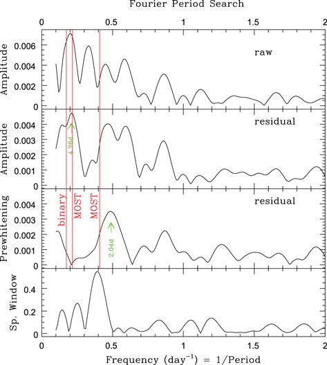
Figure 3. Periodograms derived using a Fourier period search adapted for sparse data sets. Frequencies identified in other wavelengths are shown as red vertical lines. The left red vertical line corresponds to the binary period (5.73 days), and the two strongest secondary MOST periods (4.613 and 2.448 days) are indicated by center and right red vertical lines. Top two panels: periodogram for the raw and residual data, respectively. Third panel: periodogram for the residual data after “cleaning” (prewhitening) of the strongest signal (4.76 days), leaving clearly a second period (2.04 days). Bottom panel: associated spectral window, showing the relative positions where aliases may rise.
Download figure:
Standard image High-resolution image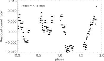
Figure 4. Residual count rate light curve of 1 ks binned data after correction for linear fit and filtering by a running median over ≈1/4d bin size. The x axis is the phase for the 4.76-day period found using period search techniques. See the text for an explanation.
Download figure:
Standard image High-resolution imageTable 3. Fourier Periods
| IDa | Period | Amp. |
|---|---|---|
| (days) | (10−3 ct s−1) | |
Raw 
|
5.0 ± 0.3 | 7.1 ± 0.7 |
| Residual | 4.76 ± 0.3 | 4.7 ± 0.08 |
| Prew. res. | 2.04 ± 0.05 | 3.5 ± 0.6 |
Note.
aRaw indicates an X-ray light curve in ; residual indicates a raw light curve with the linear trend removed; prew. res. indicates a raw light curve with the 4.76-day period and linear trend removed.
Download table as: ASCIITypeset image
The 5.0-day period in the raw data and the 4.76-day period in the residual data with the linear trend removed are considered to be the same period because the errors overlap. Comparing the periods identified in the Chandra δ Ori Aa data with the MOST optical periods, the strongest Chandra period of 4.76 days is consistent within the errors to the  period of 4.614 days (see Table 1). The Chandra period of 2.04 days is consistent with the less significant
  period of 2.138 days. There is no evidence of an X-ray period matching the binary period of 5.73 days.
Finally, we again searched for periods including the light curve from the original Chandra observation of δ Ori Aa (ObsID 639 taken in 2001). The light curve for obsid 639 alone did not yield any statistically significant periods since it covers a much smaller time interval (60 ks, hence 0.7 days). However, when combined with the 2013 data, we find similar results as mentioned above for the raw data, with a period of 5.0 days (and its harmonics at 2.5 days) providing the strongest peak. Residual light curves were not analyzed with the early observation because the linear function (which is probably not truly linear) could not be determined across an 11-year gap.
4. TIME- AND BINARY-PHASE-RESOLVED VARIABILITY
4.1. Time-sliced Spectra
The discrete photon-counting characteristic of the ACIS detector allows the creation of shorter time segments of data from longer observations. Time-resolved and phase-resolved variability of flux and emission line characteristics were investigated using a set of short-exposure spectra, contiguous in time (“time-sliced spectra”), covering the entire exposure time of the observations, along with individual instrumental responses to account for any detailed changes in local response with time, such as might be introduced by the  ks aspect dither pointing of the telescope. This was accomplished by reprocessing the set of time-sliced data using TGCat software, taking care to align the zeroth order images among the time-sliced spectra prior to the spectral extraction to produce correct energy assignments for the events. The resulting time segments are of similar exposure times,
  ks, making them easily comparable. Table 4 lists the 12 time-sliced spectra, along with the beginning and end time and binary phase range. Our Chandra observations cover parts of orbits 396–398 based on the ephemeris. The integer portion of the binary phase is in reference to the epoch of the ephemeris used. The decimal portion is the binary phase for the specific orbit.
Table 4. Chandra Time-sliced Spectra Log
| Obsid/slice | Start HJD | Start Phase | End HJD | End Phase | Duration (s) | Mid Phase |
|---|---|---|---|---|---|---|
| 14567/1 | 56280.718 | 396.606 | 56281.156 | 396.682 | 37811 | 396.644 |
| 14567/2 | 56281.156 | 396.682 | 56281.607 | 396.761 | 39000 | 396.722 |
| 14567/3 | 56281.607 | 396.761 | 56282.067 | 396.841 | 39693 | 396.801 |
| 14569/1 | 56283.267 | 397.051 | 56283.729 | 397.131 | 39948 | 397.091 |
| 14569/2 | 56283.729 | 397.131 | 56284.204 | 397.214 | 41000 | 397.173 |
| 14569/3 | 56284.204 | 397.214 | 56284.666 | 397.295 | 39906 | 397.254 |
| 14570/1 | 56285.568 | 397.452 | 56286.038 | 397.534 | 40584 | 397.493 |
| 14570/2 | 56286.038 | 397.534 | 56286.524 | 397.619 | 42000 | 397.576 |
| 14570/3 | 56286.524 | 397.619 | 56287.004 | 397.703 | 41521 | 397.661 |
| 14568/1 | 56288.177 | 397.907 | 56288.648 | 397.989 | 40662 | 397.948 |
| 14568/2 | 56288.648 | 397.989 | 56289.134 | 398.074 | 42000 | 398.032 |
| 14568/3 | 56289.134 | 398.074 | 56289.608 | 398.157 | 40941 | 398.116 |
Download table as: ASCIITypeset image
In addition to the 12 time-sliced spectra described above, we produced time-sliced spectra of approximately 10 ks in length from the Chandra observations, using the same technique described. Forty-eight time-sliced spectra with approximately 10 ks exposure times each were used in the composite spectral line analysis in Section 4.4. All other analyses used the 40 ks time-sliced spectra. We have not included the 2001 Chandra observation, obsid 639, in the following time-resolved emission-line analyses, primarily because the long-term trend of flux variability seen in our nine-day observing campaign would make the interpretation of this early observation questionable with respect to flux level.
We describe below several different analyses of the variability of the dispersed spectral data. All comparisons in this section are made to the binary orbital period, not to the periods found in the X-ray flux in Section 3, because we are interested in relating any variability to the known physical parameters of the system and possible effects of the secondary on the emission from the primary wind. First, statistical tests were performed on narrow wavelength-binned data for the 12 time-sliced spectra of 40 ks each to test for variability using  tests. We then formally fit the emission lines in each of these individual 40 ks time-sliced spectra using Gaussian profiles (Section 4.3), determining fluxes, line widths, and 1σ confidence limits. Subsequent composite line spectral analysis used the combined H-like ion profiles, as well as Fe xvii, to evaluate the flux, velocity, and line width as a function of the binary phase (Section 4.4). Finally, we looked for variability in the fir-inferred radius (Rfir) of each ion, as well as X-ray temperatures derived from the H-like to He-like line ratios (Section 4.5).
4.2. Narrow-band Fluxes and Variability
For the following statistical analysis, we used the narrow wavelength-binned bands in the 12 time-sliced, 40 ks spectra described above. The count rates for a standard set of narrow wavelength bins were output from TGCat processing. The parameters of the bins between 2.5 and 22.20 Å are listed in Table 5. We searched for variations using a series of  tests, trying several hypotheses (constancy, linear trend, and parabolic trend) and checked the improvement when more free parameters were used. The SL is defined in Section 3. Five bands were significantly variable when compared to a constant value, i.e.,
  1%: (1) the continuum centered at 4.9 Å , (2) S xv, (3) Si xiii, (4) Fe xx (10.4–12 Å ), and (5) Ne ix. A further four bands are marginally variable, i.e.,
  (1) Mg xii, (2) the continuum centered at 8.8 Å , (3) Ne x, and (4) the continuum centered at 14.925 Å . When compared to a linear trend, all but Fe xx were significantly variable, and when compared to a quadratic trend, all but Ne ix, Fe xx, and Si xiii were significantly variable, though in all cases
  %.
%.
Table 5. TGCat Wavelength Bins
| Label | λ | λ Low | λ High |
|---|---|---|---|
| (Å ) | (Å ) | (Å ) | |
| c2500a | 2.50 | 2.00 | 3.00 |
| S xvi | 4.75 | 4.70 | 4.80 |
| c4900 | 4.90 | 4.80 | 5.00 |
| S xv | 5.08 | 5.00 | 5.15 |
| c5700 | 5.70 | 5.40 | 6.00 |
| Si xiv | 6.17 | 6.10 | 6.25 |
| c6425 | 6.42 | 6.30 | 6.55 |
| Si iii | 6.70 | 6.60 | 6.80 |
| c7800 | 7.80 | 7.40 | 8.20 |
| Mg xii | 8.40 | 8.35 | 8.45 |
| c8800 | 8.80 | 8.50 | 9.10 |
| Mg xi | 9.25 | 9.10 | 9.40 |
| Fe xx | 11.20 | 10.40 | 12.00 |
| Ne x | 12.10 | 12.10 | 12.20 |
| c13200 | 13.20 | 13.00 | 13.40 |
| Ne IX | 13.60 | 13.40 | 13.80 |
| Fe xvii | 15.00 | 14.95 | 15.05 |
| c14925 | 14.92 | 14.90 | 15.05 |
| O viii | 16.00 | 15.95 | 16.05 |
| c16450 | 16.45 | 16.20 | 16.70 |
| Fe xvii | 17.07 | 17.00 | 17.15 |
| O xiii | 18.98 | 18.90 | 19.05 |
| c20200 | 20.20 | 19.20 | 21.20 |
| O vii | 21.85 | 21.50 | 22.20 |
Note.
aContinuum band labels are a “c” followed by the band wavelength in mÅ.Download table as: ASCIITypeset image
As an additional test, we directly compared the spectra one to another. Using a  test on the strongest wavelength bins, with spectra binned at 0.02 Å , variability was significant for lines (or in the regions of lines): Si xiii, Mg xii, Mg xi, Ne ix, and the zone from 10.4–12 Å (corresponding to Fe xx).
In summary, S xv, Si xiii, Ne ix, and Fe xx were variable in both of the above tests. An example of the Si xiii lines for several time slices is shown in Figure 5, demonstrating the observed variability. As noted later, Ne ix is contaminated by Fe lines, which may contribute to the variability. A few other emission lines as well as some continuum bandpasses may also be variable, but with lower confidence. As an additional confirmation of variability for one feature, Si xiii, we performed a two-sample Kolmogorov–Smirnov (KS) test (Press et al. 2002) on each time slice against the complementary data set (to ensure that the data sets are independent). With the criteria that an emission line is variable if the null hypothesis is ≤0.1, and that a line is not variable if the null hypothesis is ≥0.9, the only spectrum where the K–S test suggested real variability (at about 2% probability of being from the same distribution) was Si xiii at ϕ = 0.11. Note that the KS test shows that there is variability, but not what is varying, such as flux or centroid.
4.3. Fitting of Emission Lines
For each of the 12 time-sliced spectra of 40 ks each, the H- and He-like lines of S, Si, Mg, Ne, and O, as well as Fe xvii 15.014 Å , were fit using the Interactive Spectral Interpretation System (ISIS; Houck & Denicola 2000). Only Gaussian profiles were considered because (1) Gaussian profiles are generally appropriate at this resolution for thin winds at the signal-to-noise level of the time-sliced spectra (with some exceptions, noted below) and (2) previous studies indicated that Gaussian profiles provided adequate fits to the emission lines for both the early Chandra observation of δ Ori Aa (Miller et al. 2002) and for the combined spectrum from 2012 (Paper I). We note that lines in the spectrum of the combined HETGS data showed some deviations from a Gaussian profile (Paper I).
The continuum for each time-sliced spectrum was fit by using the same three-temperature APEC model derived in Paper I. This model allowed for line-broadening and a Doppler shift. Some abundances were fit in order to minimize the residuals in strong lines. An NH of  (Paper I) was fixed for the value of the total absorption. Only the continuum component of this model was used for continuum modeling in the following analysis.
Fits were determined by folding the Gaussian line profiles through the instrumental broadening using the RMF and ARF response functions, which were calculated individually for each time-sliced spectrum. All first order MEG and HEG counts, on both the plus and minus arms of the dispersed spectra, were fit simultaneously. For most H-like ions, the line centroid, width, and flux were allowed to vary. In a few cases where the signal-to-noise ratio (S/N) was low, the line center and/or the width was fixed to obtain a reasonably reliable fit based on the Cash statistic. For the He-like line triplets, the component lines were fit simultaneously with the line centroid of the recombination (r) line allowed to vary, and the centroids for the intercombination (i) and forbidden (f) lines forced to be offset from the r line centroid by the theoretically predicted wavelength difference. The individual flux and width values of the triplet components for the He-like ions were allowed to vary except for a few cases of low S/N when the width value of the i line and f line were forced to match that of the r line to obtain a reasonable statistical fit. The reduced Cash statistic using subplex minimization was used to evaluate each fit. For most emission lines with good signal-to-noise, the reduced Cash statistic was 0.95–1.05. A few of the lines with poor signal-to-noise had a reduced Cash statistic as low as 0.4. Confidence limits were calculated at the 68% (i.e.,  ) level for each parameter of each line, presuming that parameter was not fixed in the fit.
In most cases, the line profiles in the time-sliced spectra were well fit with a simple Gaussian. In a few cases, a profile might be better described as flat-topped with steep wings. Broad, flat-topped lines are expected to occur when the formation region is located relatively far from the stellar photosphere, where the terminal velocity has almost been reached. In such cases, Gaussian profiles are expected to fit rather poorly. Occasionally a second Gaussian profile was included for a line if a credible fit required it. If more than one Gaussian profile was used to fit a line, the total flux recorded in the data tables is the sum of the individual fluxes of the Gaussian components with the errors propagated in quadrature.
For the case of Ne ix where lines from Fe xvii and Fe xix provided significant contribution in the wavelength region of the fit, these additional Fe lines were fit separately from the Ne ix component lines. The Fe lines fit in this region were Fe xix at 13.518 Å, Fe xix at 13.497 Å, and Fe xvii at 13.391 Å, with Fe xix at 13.507 Å and Fe xix at 13.462 Å included at their theoretical intensity ratios to Fe xix at 13.518 Å. Also, the Ne x line is blended with an Fe xvii line. We have assumed that this Fe xvii component contributes flux to the Ne x line equal to 13% of the Fe xvii at 15.014 Å (Walborn et al. 2009). A final correction was applied to the Si xiii-f line because the Mg Lyman series converges in this wavelength region. Using theoretical relative line strengths, we assumed the Si xiii-f line flux was overestimated by 10% of the measured flux of the Mg xii Lα line.
Table 6. Emission Line Fluxes: S and Si
| Binary Phase | S xvi | S xv | Si xiv | Si xiii | ||||
|---|---|---|---|---|---|---|---|---|
| r | i | f | r | i | f | |||
| 0.606–0.682 |

|

|

|

|

|

|

|

|
| 0.682–0.761 |

|

|

|

|

|

|

|

|
| 0.761–0.841 |

|

|

|

|

|

|

|

|
| 0.051–0.131 | 0.1
|

|

|

|

|

|

|

|
| 0.131–0.214 | 0.6
|

|

|

|

|

|

|

|
| 0.214–0.295 |

|

|

|

|

|

|

|

|
| 0.452–0.534 |

|

|

|

|

|

|

|

|
| 0.534–0.619 |

|

|

|

|

|

|

|

|
| 0.619–0.703 |

|

|

|

|

|

|

|

|
| 0.907–0.989 |

|

|

|

|

|

|

|

|
| 0.989–0.074 |

|

|

|

|

|

|

|

|
| 0.074–0.157 | 1.8
|

|

|

|

|

|

|

|
Note. 10−6 photons s−1 cm−2. Listed in time order.
Download table as: ASCIITypeset image
Table 7. Emission Line Fluxes: Mg and Ne
| Binary Phase | Mg xii | Mg xi | Ne x | Ne ix | ||||
|---|---|---|---|---|---|---|---|---|
| r | i | f | r | i | f | |||
| 0.606–0.682 |

|

|

|

|

|

|

|

|
| 0.682–0.761 |

|

|

|

|

|

|

|

|
| 0.761–0.841 |

|

|

|

|

|

|

|

|
| 0.051–0.131 |

|

|

|

|

|

|

|

|
| 0.131–0.214 |

|

|

|

|

|

|

|

|
| 0.214–0.295 |

|

|

|

|

|

|

|

|
| 0.452–0.534 |

|

|

|

|

|

|

|

|
| 0.534–0.619 |

|

|

|

|

|

|

|

|
| 0.619–0.703 |

|

|

|

|

|

|

|

|
| 0.907–0.989 |

|

|

|

|

|

|

|

|
| 0.989–0.074 |

|

|

|

|

|

|

|

|
| 0.074–0.157 |

|

|

|

|

|

|

|

|
Note. 10−6 photons s−1 cm−2. Listed in time order.
Download table as: ASCIITypeset image
The flux values and confidence limits are tabulated in Table 6 for S and Si lines, Table 7 for Mg and Ne lines, and Table 8 for O and Fe xvii lines. To summarize the results, Figure 6 shows a comparison of the fluxes of the H-like ions. The error bars for S xvi are quite large. Si xiv shows a peak at about ϕ = 0.0 and a somewhat lower value at about ϕ = 0.6. Mg xii, Ne x, and O viii are essentially constant. Figure 7 shows the fluxes for the He-like r lines. S xv-r has a maximum at about ϕ = 0.1, with lower flux in the range ϕ = 0.5–0.8. The flux values for Si xiii-r are larger for ϕ = 0.0–0.4 than for the range ϕ = 0.5–0.8. O vii-r shows an apparent increase in flux in the ϕ = 0.5–0.7 range. Mg xi-r and Ne ix-r are relatively constant. Ne ix was consistently variable in the narrow-band statistical tests. In this Gaussian fitting of the lines, we have fit and removed the contaminating Fe lines in Ne ix, possibly removing the source of variability in this triplet. We note that the points in Figures 6 and 7 are from three different orbits of the binary. The increase in flux with time discussed in Section 3 has not been taken into account in these fitted line fluxes, either in the plots or the data tables, so care must be taken in their interpretation.
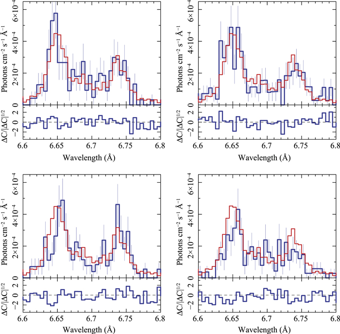
Figure 5. Si xiii profile (blue) overplotted with the mean Si xiii profile (red) of all time-sliced spectra. Upper left panel: phase is centered at 0.091 and is 0.15 wide; Upper right panel: phase is centered at 0.254 and is 0.15 wide; Lower left panel: phase is centered at 0.576 and is 0.15 wide; lower right panel: phase is centered at 0.644 and is 0.15 wide.
Download figure:
Standard image High-resolution image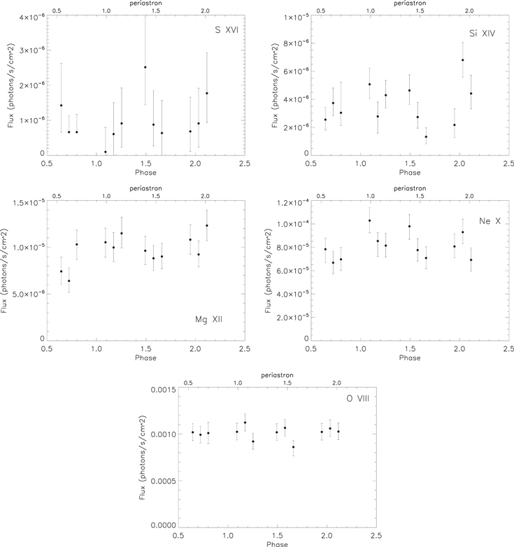
Figure 6. Flux of H-like emission lines based on Gaussian fits vs. phase. Errors are 1σ confidence limits. Phase with respect to periastron is indicated at the top of the plot.
Download figure:
Standard image High-resolution image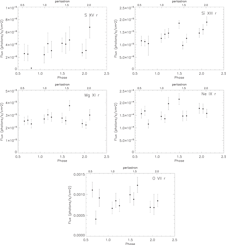
Figure 7. Fluxes of He-like r emission lines based on Gaussian fits vs. phase. Errors are 1σ confidence limits.
Download figure:
Standard image High-resolution imageTable 8. Emission Line Fluxes: O and Fe xvii
| Binary Phase | O viii | O vii | Fe xvii | ||
|---|---|---|---|---|---|
| r | i | f | |||
| 0.606–0.682 |

|

|

|

|

|
| 0.682–0.761 |

|

|

|

|

|
| 0.761–0.841 |

|

|

|

|

|
| 0.051–0.131 |

|

|

|

|

|
| 0.131–0.214 |

|

|

|

|

|
| 0.214–0.295 |

|

|

|

|

|
| 0.452–0.534 |

|

|

|

|

|
| 0.534–0.619 |

|

|

|

|

|
| 0.619–0.703 |

|

|

|

|

|
| 0.907–0.989 |

|

|

|

|

|
| 0.989–0.074 |

|

|
750.0
|

|

|
| 0.074–0.157 |

|

|

|

|

|
Note. 10−6 photons s−1 cm−2. Listed in time order.
Download table as: ASCIITypeset image
4.4. Spectral Template and Composite Line Profile (CLP) Fitting
In order to improve the S/N in line fits in the time-sliced data, we used two methods to fit multiple lines simultaneously. In the first method, we adopted a multithermal APEC (Smith et al. 2001; Foster et al. 2012) plasma model that describes the mean spectrum fairly well (see Table 9), and used this as a spectral template, allowing the fits to the Doppler shift, line width, and overall normalization to vary freely. This is a simpler model than the more physically based APEC model defined in Paper I since here it need not fit the spectrum globally, but is only required to fit a small region about a feature of interest. To demonstrate this, Figure 8 shows an example after fitting only the 8.3– region for the Mg xii feature’s centroid, width, and normalization for the entire exposure. The temperatures were not varied, and the relative normalizations of the three components were kept fixed, as was the absorption column. We can see that this provides a good local characterization of the spectrum, and so will be appropriate for studying the variations of these free parameters in local regions as a function of time or phase. For any such fit, other regions will not necessarily be well described by this model.
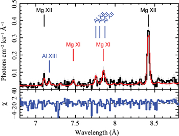
Figure 8. Portion of the HEG spectrum for the entire exposure, after fitting an APEC template to the 8.3– region. The temperatures, relative normalizations, and absorption were frozen parameters. The Doppler shift, line width, and normalization were free. We show the resulting model evaluated over a broader region that was fitted to demonstrate the applicability of the model to the local spectral region. Other regions will not necessarily be well represented by the same parameters.
Download figure:
Standard image High-resolution imageTable 9. Plasma Model Parameters Used for Spectral Template Fitting
| Temperature Componentsa | |
|---|---|
| T | Norm |
| 2.2 | 8.16 |
| 6.6 | 1.90 |
| 19.5 | 0.226 |
| Relative Abundancesb | |
| Elem. | A |
| Ne | 1.2 |
| Mg | 0.7 |
| Si | 1.6 |
| Fe | 0.9 |
| Total Absorptionc | |
| NH | 0.15 |
Note.
aTemperatures are given in MK, and the normalization is related to the volume emission measure, VEM, and distance, d, via
 .
bWe give elemental abundances relative to the solar values of Anders & Grevesse (1989) for those significantly different from 1.0. (These are not rigorously determined abundances, but related to discrete temperatures adopted and actual abundances.).
cThe total absorption is given in units of
.
bWe give elemental abundances relative to the solar values of Anders & Grevesse (1989) for those significantly different from 1.0. (These are not rigorously determined abundances, but related to discrete temperatures adopted and actual abundances.).
cThe total absorption is given in units of  .
.
Download table as: ASCIITypeset image
These fits used spectra extracted in 10 ks time bins (about 0.02 in phase), but were fit using a running average of three time bins. We primarily used the H-like  lines, as well as some other strong and relatively isolated features (see Table 10). The results for the interesting parameters, the mean Doppler shift of the lines and their widths, are shown in Figure 9. The smooth curve in the top panel is the binary orbital radial velocity curve. We clearly see a dip in the centroid near
  , as well as significant changes in average line width.
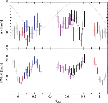
Figure 9. Mean emission line Doppler velocity (top, points with error bars), primary radial velocity (top, sinusoidal curve), and mean line width for Ne x (bottom) derived by fitting spectra in phase bins with an APEC template, allowing the Doppler shift, line width, and normalization to vary freely. Data from the individual Chandra observations are differentiated with colors. Error bars (1σ) are correlated over several bins since a running average was used over 3–10 ks bins.
Download figure:
Standard image High-resolution imageTable 10. Lines Used in CLP Analysisa

|
Feature |
|---|---|
| Å | |
| 6.182 | Si xiv |
| 8.421 | Mg xii |
| 10.239 | Ne x |
| 11.540 | Fe xviii |
| 12.132 | Ne x |
| 14.208 | Fe xviii |
| 15.014 | Fe xvii |
| 15.261 | Fe xvii |
| 16.005 | Fe xviii+O viii |
| 16.780 | Fe xvii |
| 17.051 | Fe xvii |
| 18.968 | O viii |
Note.
aLines used in the ensemble fitting with Composite Line Profile or spectral template methods. Both HEG and MEG were used at wavelengths shorter than 16 Å . The region widths were 0.20 Å , centered on each feature.Download table as: ASCIITypeset image
In the second method, we rebinned regions around selected features to a common velocity scale and summed them into a “CLP.” While this mixes resolutions (the resolving power is proportional to wavelength and is different for HEG and MEG) and blends in the CLP, the mix should be constant with phase and be sensitive to dynamics as long as line ratios themselves do not change. Hence, we can search for phased variations in the line centroid. This technique has been applied fruitfully in characterizing stellar activity in cool stars (Hoogerwerf et al. 2004; Huenemoerder et al. 2006). The CLP profiles were computed in phase bins of 0.01, but grouped by 5 bins for fitting, thus forming a running average. We used the same lines as in the template fitting. In Figure 10, we show an example of CLPs, and fits of a Lorentzian (since the composite profile is no longer close to Gaussian) plus a polynomial to determine centroid and width. This method, while less direct than template fitting, did confirm the trend seen in line velocity in the template fitting.
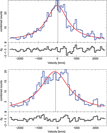
Figure 10. Example of Composite Line Profiles for two different phases with different centroids, 0.68 (top) and 0.78 (bottom), as defined by the photometric ephemeris. In each large panel, the histogram is the observed profile, the smooth curve is the fit. In the small panel below each are the residuals.
Download figure:
Standard image High-resolution imageThe template-fit line width result is very interesting in that it shows a significantly narrower profile near  than at other phases. Given the trends in width, (low near phase 0.0, high near 0.2 and 0.8) 10 ks time-sliced spectra were grouped in these states and then compared (Figure 11). The plots show the narrow state in blue and the broad state in red. The lines are all sharper, except for the line at 17 Å (and maybe Si xiv 6 Å ), in the narrow state. The top panel of Figure 11 shows a heavily binned overview, and the lower panel shows a comparison of the Ne x line profiles at ϕ = 0 and at quadrature phases.
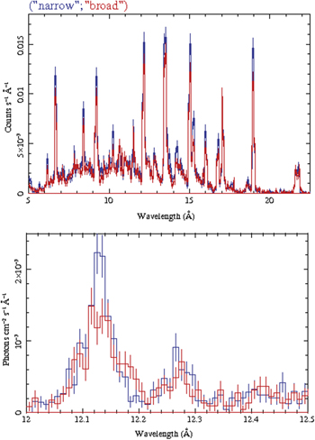
Figure 11. Examples of broad and narrow emission lines for selected wavelength regions. Plots are constructed from counts per bin data without continuum removal. For this comparison, the 10 ks time-sliced spectra have been combined to represent ϕ = 0.0 (blue) and the quadrature phases (red).
Download figure:
Standard image High-resolution imageThe line width variability was confirmed by comparing the average spectrum at phases near  with the average spectrum at other phases. The changes were primarily in a reduced strength of the line core in the phases when the lines are broad, with little or no change in the wings.
Figure 12 shows the trend versus emission line. Except for Ne x and Fe xvii 17 Å , there is a trend for larger differences in the FWHM with increasing wavelength. Note that the temperature of maximum emissivity goes roughly inversely with wavelength; wind continuum opacity increases with wavelength. The increasing trend is typical of winds, since the opacity causes longer wavelength lines to be weighted more to the outer part of the wind where the velocity is higher. Gaussian fit centroids show that the lines are all slightly blueshifted, which could be consistent with skewed wind profiles. The “narrow” group is near the primary star radial velocity shift. Radial velocities of the lines are all roughly consistent with −80 km s−1, except perhaps Ne x, which is blended with an Fe line. The dependence between line width and binary phase was confirmed independently by moment analyses of the individual lines, and was also suggested by the CLP analysis above.
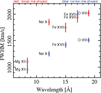
Figure 12. Comparison of FWHM in km s−1 for several emission lines in the time-sliced spectra of δ Ori Aa. For this comparison, the 10 ks time-sliced spectra have been combined to represent ϕ = 0.0 (blue) and the quadrature phases (red). Note that these spectra do not have continuum removal. Gaussian plus polynomial line fitting was used on the time slices to determine the line width.
Download figure:
Standard image High-resolution image4.5. X-Ray Emission Line Ratios
The He-like ions provide key plasma diagnostics using the relative strengths of their fir (forbidden, intercombination, resonance) lines by defining two ratios:19
the R ratio =  and the G ratio =
  . Gabriel & Jordan (1969) demonstrated that the
  and G ratios are sensitive to the X-ray electron density and temperature, respectively. These ratios have been used extensively in stellar X-ray studies. In addition, the presence of a strong UV/EUV radiation field can change the interpretation of the
  ratio from a density diagnostic to a measurement of the radiation field geometric dilution factor, i.e., effectively the radial location of the X-ray emission from a central radiation field (Blumenthal et al. 1972). The
  ratio is known to decrease in the case of a high electron density and/or high radiation flux density, which will depopulate the upper level of the f-line transition (weakening its emission) while enhancing the i-line emission. For hot star X-ray emission, the
  ratio is controlled entirely by the strong UV/EUV photospheric radiation field. The first analysis of an O supergiant HETG spectrum by Waldron & Cassinelli (2001) verified that the observed X-ray emission is distributed throughout the stellar wind and demonstrated that density effects could only become important in high energy He-like ions if their X-rays are produced extremely close to the stellar surface. Thus the
  ratio can be exploited to determine the onset radius or the fir-inferred radius (Rfir in units of
  ) of a given ion via the geometric dilution factor of the photospheric radiation field (Waldron & Cassinelli 2001). In addition, there are basically two types of fir-inferred radii, “localized” (point-like) or “distributed.” The first detailed distributed approach was developed by Leutenegger et al. (2006) assuming an X-ray optically thin wind. For a given observed
  ratio, the localized approach predicts a larger Rfir as compared to the distributed approach (see the discussion in Waldron & Cassinelli 2007). Since all X-ray emission lines scale as the electron density squared, all line emissions are primarily dominated by their densest region of formation. However, in the case of the fir lines, an enhanced i-line emission can only occur deep within the wind (high density), whereas the majority of the f-line emission is produced in the outer wind regions at lower densities. The r-line emission is produced throughout the wind.
Another X-ray temperature-sensitive line ratio is the H-like to He-like line ratio (H/He) as explored in several hot-star studies (e.g., Miller et al. 2002; Schulz et al. 2002; Waldron et al. 2004; Waldron & Cassinelli 2007). However, a wind distribution of X-ray sources implies a density dependence (i.e., the H-like and He-like lines may be forming in different regions) and a dependence on different wind X-ray absorption effects. Thus, the temperatures derived from H/He ratios may be higher than their actual values (see Waldron et al. 2004; Waldron & Cassinelli 2007).
Our line ratio analysis is based on the approach given by Waldron & Cassinelli (2007). The  ratios for each He-like ion in each time-sliced spectrum are tabulated in Tables 11–14. We did not include S in this analysis because the flux measurement errors are large and the flux ratio errors are extremely large or unbounded. We calculated the fir-inferred radii (Rfir) and H/He-inferred temperatures (THHe) versus phase for the 12 time-sliced spectra, as determined by the Gaussian line fitting. All radii were determined by the point-like approach and a TLUSTY photospheric radiation field with parameters Teff = 29,500 kK and log G = 3.0. The model
  ratios and H/He ratios used to extract Rfir and THHe information take into account the possible contamination from other lines. For all derived Rfir, we assume that the He-like ion line temperature is at its expected maximum value.
Table 11. Silicon Line Ratios and Derived Parameters
| Phase | MJD |
 Ratio Ratio |
G Ratio |
 Ratio Ratio |

|
TG MK | THHe MK |
|---|---|---|---|---|---|---|---|
| Time Ordered | |||||||
| .646 | 56280.93 | 0.52 ± 0.26 | 0.41 ± 0.12 | 0.25 ± 0.09 |

|
⋯ | 8.23 ± 0.79 |
| .734 | 56281.38 | 1.30 ± 0.46 | 0.83 ± 0.17 | 0.38 ± 0.11 | 1.46 ± 0.41 |

|
9.36 ± 0.83 |
| .777 | 56281.84 | 0.73 ± 0.37 | 1.47 ± 0.72 | 0.41 ± 0.24 | 1.10 ± 0.09 | 6.45 ± 3.99 | 9.27 ± 1.66 |
| .082 | 56283.49 | 1.19 ± 0.35 | 0.94 ± 0.19 | 0.44 ± 0.11 | 1.32 ± 0.28 | 7.16 ± 3.36 | 9.73 ± 0.74 |
| .170 | 56283.97 | 3.21 ± 1.14 | 0.87 ± 0.20 | 0.20 ± 0.09 |

|
10.20 ± 6.18 | 7.82 ± 0.87 |
| .257 | 56284.44 | 1.99 ± 0.96 | 0.42 ± 0.09 | 0.32 ± 0.08 |

|
⋯ | 8.93 ± 0.70 |
| .475 | 56285.79 | ⋯ | 0.49 ± 0.09 | 0.28 ± 0.07 | ⋯ | ⋯ | 8.60 ± 0.57 |
| .562 | 56286.28 | 1.42 ± 0.40 | 1.25 ± 0.25 | 0.32 ± 0.11 | 1.56 ± 0.42 | 3.73 ± 0.83 | 8.90 ± 0.94 |
| .649 | 56286.77 | 2.19 ± 0.77 | 0.94 ± 0.19 | 0.12 ± 0.05 |

|
7.13 ± 3.38 | 6.99 ± 0.59 |
| .955 | 56288.40 | 3.95 ± 2.29 | 0.57 ± 0.14 | 0.17 ± 0.08 |

|

|
7.49 ± 0.83 |
| .042 | 56288.89 | 2.91 ± 1.14 | 0.83 ± 0.16 | 0.46 ± 0.10 |

|
11.11 ± 6.39 | 9.86 ± 0.63 |
| .129 | 56289.38 | 0.99 ± 0.22 | 0.73 ± 0.11 | 0.25 ± 0.07 | 1.14 ± 0.13 |

|
8.31 ± 0.63 |
Note. Null entries imply unresolved ratio and/or parameter ranges.
Download table as: ASCIITypeset image
Table 12. Magnesium Line Ratios and Derived Parameters
| Phase | MJD |
 Ratio Ratio |
G Ratio |
 Ratio Ratio |

|
TG MK | THHe MK |
|---|---|---|---|---|---|---|---|
| Time Ordered | |||||||
| .646 | 56280.93 | 0.54 ± 0.13 | 0.94 ± 0.16 | 0.32 ± 0.07 | 2.30 ± 0.34 | 4.35 ± 1.64 | 5.71 ± 0.36 |
| .734 | 56281.38 | 0.66 ± 0.19 | 0.93 ± 0.18 | 0.27 ± 0.06 | 2.61 ± 0.49 | 4.82 ± 2.12 | 5.46 ± 0.31 |
| .777 | 56281.84 | 0.51 ± 0.15 | 1.02 ± 0.21 | 0.48 ± 0.10 | 2.20 ± 0.41 | 3.86 ± 1.50 | 6.33 ± 0.33 |
| .082 | 56283.49 | 0.38 ± 0.11 | 0.96 ± 0.18 | 0.42 ± 0.08 | 1.85 ± 0.31 | 4.20 ± 1.63 | 6.14 ± 0.32 |
| .170 | 56283.97 | 1.26 ± 0.60 | 0.62 ± 0.16 | 0.36 ± 0.07 | 4.55 ± 1.94 | 36.40 ± 30.34 | 5.89 ± 0.36 |
| .257 | 56284.44 | 0.83 ± 0.23 | 0.86 ± 0.16 | 0.44 ± 0.08 | 3.10 ± 0.62 | 17.48 ± 14.41 | 6.21 ± 0.30 |
| .475 | 56285.79 | 1.05 ± 0.53 | 0.82 ± 0.23 | 0.38 ± 0.08 | 3.73 ± 1.49 | 25.29 ± 22.37 | 5.97 ± 0.37 |
| .562 | 56286.28 | 0.42 ± 0.13 | 0.87 ± 0.15 | 0.37 ± 0.07 | 1.97 ± 0.36 | 16.95 ± 13.89 | 5.97 ± 0.35 |
| .649 | 56286.77 | 3.05 ± 1.67 | 0.41 ± 0.09 | 0.26 ± 0.05 | 4.54 ± 0.00 |

|
5.43 ± 0.24 |
| .955 | 56288.40 | 0.68 ± 0.17 | 1.19 ± 0.21 | 0.50 ± 0.10 | 2.71 ± 0.46 | 2.68 ± 0.64 | 6.42 ± 0.28 |
| .042 | 56288.89 | 0.57 ± 0.14 | 1.11 ± 0.18 | 0.46 ± 0.09 | 2.38 ± 0.37 | 3.02 ± 0.75 | 6.27 ± 0.30 |
| .129 | 56289.38 | 0.60 ± 0.19 | 0.82 ± 0.17 | 0.44 ± 0.08 | 2.45 ± 0.50 | 20.51 ± 17.27 | 6.21 ± 0.31 |
Download table as: ASCIITypeset image
Table 13. Neon Line Ratios and Derived Parameters
| Phase | MJD |
 Ratio Ratio |
G Ratio |
 Ratio Ratio |

|
TG MK | THHe MK |
|---|---|---|---|---|---|---|---|
| Time Ordered | |||||||
| .646 | 56280.93 | 0.23 ± 0.10 | 0.60 ± 0.11 | 0.82 ± 0.12 | 3.93 ± 0.96 | ⋯ | 3.66 ± 0.17 |
| .734 | 56281.38 | 0.21 ± 0.08 | 0.80 ± 0.13 | 0.70 ± 0.10 | 3.66 ± 0.73 |

|
3.49 ± 0.14 |
| .777 | 56281.84 | 0.19 ± 0.06 | 1.55 ± 0.28 | 1.01 ± 0.17 | 3.54 ± 0.61 | 1.05 ± 0.17 | 3.89 ± 0.21 |
| .082 | 56283.49 | 0.17 ± 0.05 | 1.19 ± 0.18 | 1.07 ± 0.14 | 3.35 ± 0.60 | 1.63 ± 0.49 | 3.97 ± 0.16 |
| .170 | 56283.97 | 0.27 ± 0.11 | 0.56 ± 0.11 | 0.92 ± 0.13 | 4.24 ± 1.00 | ⋯ | 3.80 ± 0.18 |
| .257 | 56284.44 | 0.25 ± 0.12 | 0.40 ± 0.10 | 0.66 ± 0.10 | 4.02 ± 1.15 | ⋯ | 3.44 ± 0.14 |
| .475 | 56285.79 | 0.33 ± 0.11 | 0.52 ± 0.09 | 0.71 ± 0.09 | 4.86 ± 0.91 | ⋯ | 3.51 ± 0.13 |
| .562 | 56286.28 | 0.14 ± 0.08 | 0.93 ± 0.20 | 0.87 ± 0.14 | 2.89 ± 0.96 |

|
3.73 ± 0.19 |
| .649 | 56286.77 | 0.40 ± 0.10 | 0.87 ± 0.15 | 0.78 ± 0.12 | 5.39 ± 0.77 |

|
3.60 ± 0.17 |
| .955 | 56288.40 | 0.21 ± 0.06 | 0.99 ± 0.16 | 0.75 ± 0.11 | 3.65 ± 0.59 | 2.57 ± 1.05 | 3.57 ± 0.15 |
| .042 | 56288.89 | 0.31 ± 0.08 | 1.03 ± 0.15 | 0.85 ± 0.11 | 4.74 ± 0.67 | 2.26 ± 0.82 | 3.70 ± 0.16 |
| .129 | 56289.38 | 0.38 ± 0.13 | 0.54 ± 0.10 | 0.83 ± 0.11 | 5.16 ± 0.96 | ⋯ | 3.67 ± 0.15 |
Note. Null entries imply unresolved ratio and/or parameter ranges.
Download table as: ASCIITypeset image
Table 14. Oxygen Line Ratios and Derived Parameters
| Phase | MJD |
 Ratio Ratio |
G Ratio |
 Ratio Ratio |

|
TG MK | THHe MK |
|---|---|---|---|---|---|---|---|
| Time Ordered | |||||||
| .646 | 56280.93 | 0.12 ± 0.08 | 0.84 ± 0.20 | 1.05 ± 0.19 | 9.05 ± 3.40 | 3.40 ± 1.90 | 2.32 ± 0.13 |
| .734 | 56281.38 | 0.06 ± 0.05 | 2.50 ± 1.01 | 2.55 ± 0.94 | 6.29 ± 2.88 | 0.00 ± 0.62 | 2.98 ± 0.36 |
| .777 | 56281.84 |

|
0.96 ± 0.27 | 1.26 ± 0.31 |

|
2.70 ± 1.63 | 2.43 ± 0.18 |
| .082 | 56283.49 |

|
1.19 ± 0.34 | 1.73 ± 0.39 |

|
1.59 ± 0.99 | 2.68 ± 0.17 |
| .170 | 56283.97 |

|
0.83 ± 0.25 | 1.50 ± 0.32 |

|
4.73 ± 3.32 | 2.56 ± 0.16 |
| .257 | 56284.44 |

|
0.90 ± 0.27 | 1.43 ± 0.31 |

|
3.31 ± 2.14 | 2.52 ± 0.16 |
| .475 | 56285.79 |

|
0.74 ± 0.23 | 1.17 ± 0.25 |

|

|
2.39 ± 0.15 |
| .562 | 56286.28 |

|
0.68 ± 0.18 | 1.37 ± 0.26 |

|

|
2.50 ± 0.14 |
| .649 | 56286.77 | 0.09 ± 0.08 | 0.36 ± 0.11 | 0.79 ± 0.14 | 6.52 ± 3.89 |

|
2.15 ± 0.09 |
| .955 | 56288.40 |

|
1.11 ± 0.30 | 1.66 ± 0.35 |

|
1.78 ± 1.07 | 2.64 ± 0.16 |
| .042 | 56288.89 | 0.05 ± 0.05 | 0.97 ± 0.45 | 1.60 ± 0.53 | 5.26 ± 3.31 |

|
2.59 ± 0.26 |
| .129 | 56289.38 |

|
0.83 ± 0.22 | 1.38 ± 0.27 |

|
3.70 ± 2.22 | 2.50 ± 0.14 |
Download table as: ASCIITypeset image
The fir-inferred radii for Mg and Si are plotted in Figure 13 and for Ne and O in Figure 14. In all cases the derived Rfir is based on the average of the minimum and maximum predicted values, so if the lower bound is at one, then the upper bound should be considered as an upper limit. In these plots, any lower limits are indicated by arrows. The binary phase is used for the x axis. There are 10 cases showing a finite range for the O Rfir. There are two O and Ne Rfir values at phase  , but in different binary orbits, indicating the same finite radial locations (within the errors) for each ion (O at
  , and Ne at
  ), which could mean that at least for O and Ne the behavior is repeatable. This is not seen in Mg or Si. For Mg, in one case for
  there is a finite Rfir (≈2), whereas the other case at
  indicates only a lower bound of ≈4.5. For Si there are five Rfir with finite ranges, all within the errors of one another. Si has four Rfir at
  since the observed
  for these phases were below their respective minimum
  . This behavior suggests that these regions producing the majority of the higher energy emission lines may be experiencing significant dynamic fluctuations in density and/or temperature.
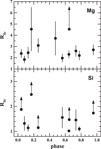
Figure 13. Phase dependence of the derived Mg and Si fir-inferred radii (Rfir) for the 12 time-sliced spectra. Upper and lower limits are shown as arrows. See the text for model details.
Download figure:
Standard image High-resolution image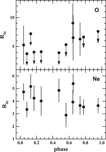
Figure 14. Phase dependence of the derived O and Ne fir-inferred radii (Rfir) for the 12 time-sliced spectra. Upper and lower limits are shown as arrows. See the text for model details.
Download figure:
Standard image High-resolution imageThe 12 derived H/He temperatures (THHe) versus phase for each ion are shown in Figure 15. In general, for all ions there is very little variation in THHe with phase, though one could easily argue that at certain phases there are minor fluctuations.
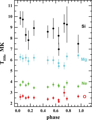
Figure 15. Phase dependence of the Si, Mg, Ne, and O THHe calculated from the H/He ratios of each of the twelve 40 ks time-sliced spectra.
Download figure:
Standard image High-resolution imageA verification of these results was obtained using the Potsdam Wolf–Rayet code (Hamann & Gräfener 2004) to perform a similar  analysis that included diffuse wind emission and limb darkening. Differences in the results obtained using the two methods were negligible compared to measurement uncertainties.
4.6. Non-detection of Stellar Wind Occultation Effects
One goal of this program was to use the variable occultation of the primary wind by the essentially X-ray-dark secondary, δ Ori Aa2, as it orbits the primary, mapping the ionization, temperature, and velocity regimes within the primary’s stellar wind. The secondary star, δ Ori Aa2, is orbiting deep within the wind of the primary star, δ Ori Aa1. Based on the binary separation of 2.6  and our calculations of the fir-inferred radii of the various ions, we expect the secondary to be outside of the onset radius of S emission in the primary wind, very close to, or inside of, the onset radius of Si, and inside the onset radii of Mg, Ne, and O. We can make a simple model of the expected light curves for these emission lines for δ Ori Aa. If the secondary is outside of the onset radius of an ion, the light curve will have a maximum and relatively constant flux value between ϕ ≈ 0.25 and ≈0.75. The light curve will have a relatively constant but lower flux at ϕ ≈ 0.75–0.25 as it occults both the back and front sides of the onset-radius shell. If the secondary is inside the onset radius of an ion, then the light curve will be at a maximum flux near ϕ = 0.0 and 0.5. Between these two phases, the light curve will have a lower and relatively constant flux value as it occults only the back side of the onset-radius shell.
The i line of the He-like triplet is formed deep in the wind while both the r and f lines are more distributed throughout the wind. Our best chance of identifying occultation effects is probably from the fluxes of the i lines, as the shell of i-line emission will be thinner than either the f-line emission shell or the r-line emission shell. To estimate any occultation effect that we might see in these light curves, we calculated the maximum volume of i-line emission that could be occulted by the secondary using various parameters. The total i-line emission expected from an emitting shell around the surface of the star was estimated using the spherical volume of the shell. The secondary star is assumed to have a radius of 0.3 RAa1. The percentage of i-line emission occulted by the secondary star will be maximum when the largest column of emitting material is occulted, which is at the rim of the shell. An estimate of the occulted emission was based on the volume of the spherical cap of the emitting shell, with a height equal to the diameter of the secondary star. Care was taken to subtract the volume of the star that might be included in the cap. We find that, for the extreme case of an i-line emission shell at the surface of the primary star with a thickness of 0.01  , the maximum occultation of the i-line flux would reduce the flux by ≈20%. If the thickness of the i-line shell is instead a more likely value of 0.1 RAa1 but still in contact with the surface of the star, the flux of the i emission line would be reduced by only about 3% due to occultation by the secondary. In these estimates, the secondary would not be at primary minimum ϕ = 0.0, but instead projected on the rim of the i-line emission shell where the column of i-line emission is greatest. A thicker i-line shell would reduce the amount of occultation further because of the finite size of the projected secondary star in relation to the volume of the sphere of i-line emission. Any other position of the secondary in the orbit, or any larger shell of i-line emission, would reduce the percentage of occultation.
Figure 16 shows the flux measurements for the i lines of the He-like triplets. We have previously found a linear increase in flux over the time period of the observations which is not removed in these plots. While the estimates of the fluxes from the S xv-i and Si xiii-i lines that might have an onset radius very close to the stellar surface of the primary star do not preclude the existence of occultation effects, we unfortunately cannot identify such variability which would be at the 1%–2% level, particularly due to the other identified variations on the order of 10%–15% and the errors of the measurements.
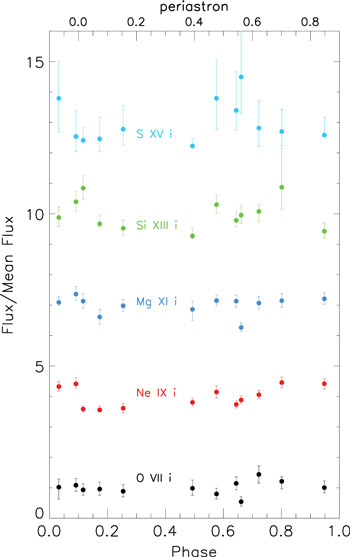
Figure 16. Flux of the He-like i component of the triplet based on Gaussian fits vs. phase. The errors are 1σ confidence limits. The fluxes have been normalized by dividing by the mean flux for the respective line. The phase with respect to the periastron is indicated at the top of the plot. The plot for each ion is offset by a value of three from the previous one for clarity.
Download figure:
Standard image High-resolution image5. DISCUSSION
5.1. Effects of a Wind–Star Collision
An important and unexpected result of this analysis is the discovery of the variability of line widths with binary phase. H-like emission line widths are at a minimum at ϕ = 0.0 when the secondary is in front of the primary, and to a lesser degree at ϕ = 0.7. The line widths are at a maximum near ϕ = 0.2 and ϕ = 0.8, close to quadrature. The phase-dependent variability of the emission line widths must therefore be related to interaction between the primary and the secondary.
In Paper I, we developed a model to represent the effect of the secondary star on the wind region of the primary. Our 1D, line-of-centers, CAK calculations presented in Paper I showed that radiative braking does not occur in this system, so the primary wind directly impacts the surface of the secondary star. A similar example has been observed for CPD  7742, along with an eclipse of the X-ray emitting colliding wind region when the two stars were perfectly aligned (Sana et al. 2005). A 3D smoothed particle hydrodynamics (SPH) code (Madura et al. 2013; Russell 2013) was then used to simulate the effect of the wind–wind collision in δ Ori Aa. The colliding winds form an approximately cone-shaped cavity in the wind of the primary with the secondary star at the apex of the cone. The cavity has a half-opening angle of ≈30°, so the solid angle fraction taken up by the cone is ≈8%. A bow shock surrounds the cavity, and within this cavity the secondary wind prevails, yielding lower densities as well as very little X-ray flux. Figure 17, reproduced from Paper I, shows the density and temperature structure of the winds and their interaction in the binary orbital plane. The hot gas in the shock at the interface between the lower density cavity and the primary star wind was calculated in Paper I to produce at most 10% of the observed X-ray flux. According to this model, as the cavity rotates around the primary star from the blue- to redshifted part of the wind, emission line profiles should change in shape and velocity (as long as the radius of line formation is similar to, or larger than, the location of the apex of the bow shock).
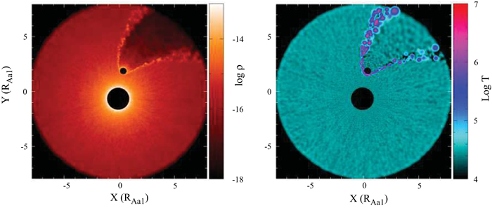
Figure 17. Model of density and temperature structure of the binary orbital plane of the SPH simulation of Aa1 (larger black circle) and Aa2 (smaller black circle), based on the parameters from Paper IV and the model in Paper I. The collision of the wind of the primary star against the secondary star produces a low density cavity within the primary wind. The perimeter of the low density cavity is a shocked bow shock of higher density than either star’s wind region (left panel). In the temperature plot on the right, only the hot gas from along the wind-collision, bow shock boundary is shown since the SPH simulation does not include the embedded wind shocks of either δ Ori Aa1 or δ Ori Aa2. The primary wind collides directly with the secondary surface in this simulation primarily because of the large difference in the mass-loss rate ( ).
).
Download figure:
Standard image High-resolution imageThe variability of the emission-line widths we have observed may potentially be explained by this cavity in the primary wind caused by the wind interaction with the secondary. When viewed at ϕ = 0.0, the cavity will occupy a region of the primary stellar wind that would otherwise be the formation region of emission with high negative velocities. The emission line profiles viewed at this phase might then be truncated at the largest negative velocities, creating a comparatively narrower profile than one expects without the presence of the secondary. At ϕ = 0.5, some of the most positive velocities would not be detected in the emission-line profiles. Wind absorption must be taken into account at ϕ = 0.5 and the effect of the cavity may be less pronounced. Such emission truncation at ϕ = 0.0 and 0.5 is suggested in Figure 18, displaying the Mg xii profiles and fits for the time-sliced spectrum near ϕ = 0.0 and the time-sliced spectrum near ϕ = 0.5. The Mg xii line was chosen as a relatively strong line that was also used in the template analysis in Section 4.4. The red line in the figure is the Gaussian fit to the line, the black line is the time-sliced spectrum for a particular phase interval, and the lower panel of each plot shows the  statistic (though the Cash statistic was actually used in the fitting). Negative velocities appear somewhat under-represented in the time-sliced spectrum near ϕ = 0.0, though the profile near ϕ = 0.5 does not appear to be asymmetric. There could be other explanations for this characteristic, such as velocity changes in the centroid or non-Gaussian profiles. At quadrature, ϕ = 0.25 and 0.75, the velocities normally produced in the embedded wind of the primary and replaced by the region occupied by the cavity will tend to be near zero velocity, resulting in emission lines of expected widths, but somewhat non-Gaussian peaks, such as flat-topped or skewed peaks. This prediction is not inconsistent with the profiles observed near quadrature in the δ Ori Aa time-sliced spectra, which are broader than the profiles seen near conjunction (see Figure 18 as an example).
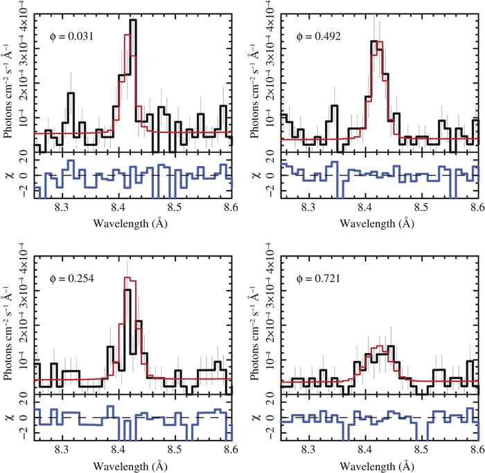
Figure 18. Mg xii profile overplotted with the Gaussian fit. Upper left panel: phase is centered at 0.031. Upper right panel: phase is centered at 0.492. Lower left panel: phase is centered at 0.254. Lower right panel: phase is centered at 0.721.
Download figure:
Standard image High-resolution imageHowever, further analysis of the Mg xii line reveals a more complex scenario. Figure 19 shows the correlation of FWHM with flux for Mg xii for the 12 time-sliced spectra, based on the Gaussian fits. While most of the points show a similar distribution with little or no dependence of FWHM on flux, the three points from the first Chandra observation, ObsID 14567, have significantly larger FWHM values along with lower flux. We have carefully checked that there is no known reason to expect this result to be instrumental. We conclude that the variability in the Mg xii line has several timescales, of which the binary orbit and colliding winds associated with the binary system are only one component.
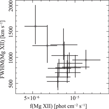
Figure 19. Gaussian parameters for Mg xii lines for each of the 12 time-sliced spectra. Error bars are 1σ. Flux vs. FWHM.
Download figure:
Standard image High-resolution image5.2. Stellar Pulsations and Corotation Interacting Regions
Pulsations have been found in only a few O stars, but those that have been found are mostly in late-O stars, such as ζ Oph, O9.5 V (Walker et al. 2005). Variations due to pulsations are cyclic, even over long timescales (i.e., Prinja & Howarth 1986; Henrichs et al. 1988; Prinja 1988; Massa et al. 1995; Kaper et al. 1996, 1997, 1999). Models predict that massive stars near the main sequence will experience pulsations of several types, including non-radial pulsations (NRP), β Cep instabilities, and l-mode pulsations (Cox et al. 1992; Pamyatnykh 1999).
Another source of variability relates to phenomena near or on the surface of the star, such as bright spots, which tend to be transient over a few stellar rotations or less. For many years DAC variability in UV P-Cygni profiles has been recognized, and is believed to be common in O stars. Cranmer & Owocki (1996) provided a model of ad hoc photospheric perturbations in the form of bright spots that was able to reproduce the DAC phenomenon. CIRs, possibly related to DACs, are perturbations that start at the base of the stellar wind and can extend far out into the wind, and thus are tied to the rotation period of the star, although they could also be transient. Presumably there can be multiple CIRs distributed over the surface of the star, cumulatively resulting in variations that appear to be shorter than the rotation period, although each individual spot and its associated CIR will rotate with the star.
The periods we have identified in the Chandra light curve of δ Ori Aa (4.76 and 2.04 days, see Section 3), are possibly the X-ray signature of CIRs or pulsations. The 4.76 ± 0.3 day period may be the rotation period of the primary star. Based on a  value of 130 km s−1 (Paper IV) and the estimated value of R
 = 12R⊙, and also including the assumption of alignment between the rotational and orbital axes, the rotational period should be about 4.7 days, consistent with our strongest period of 4.76 days. A single non-transient CIR would share the stellar rotational period. We did not find evidence of the binary orbital period of 5.73 days in the X-ray light curve, indicating that most of the X-ray variability is not related to the orbital motion, at least for the limited orbital data we have.
There is an apparent increase in flux over nine days, suggesting long-term variability. We do not have a sufficient time baseline to quantify this component of variability, but it is clearly not associated with the binary period. We suggest that this long-term variability is due to pulsations such as NRP and/or increasing CIR activity.
6. CONCLUSIONS
Chandra high-resolution grating X-ray spectra of δ Ori Aa acquired in 2012 with a total exposure time of  ks have been analyzed for phase-resolved and time-resolved variability. Several components of variability were detected in our analyses.
The count rate of the entire spectral range increased during the nine-day observing campaign by approximately 25%. We cannot constrain the cause of this longer-term variability with this data set, but we speculate that this may be related to stellar pulsations or CIRs and other wind instabilities.
An important result of the period searches in the X-ray data is that the binary motion seems to contribute very little to the variability of the total flux. A period search of the total X-ray flux light curve yielded periods of 4.76 ± 0.3 days and 2.04 ± 0.5 days after removal of the long-term trend, both of which are less than the binary period of 5.73 days. A period search including the early 2001 Chandra observation as well as the 2012 data gave a period near 5.0 days, within the errors of the 4.76-day period determined from the normalized 2012 spectra. The 4.76-day period is consistent with the secondary period found by MOST of 4.614 days; thus it is present in both X-ray and optical data. We suggest that this may be the rotation period of δ Ori Aa1 based on estimates of  and the radius of δ Ori Aa1. The 2.04-day period, also found in the MOST photometry, may be associated with pulsations or CIRs.
Flux variability of individual emission lines was confirmed with statistical tests for the He-like triplets of S xv, Si xiii, and Ne ix (contaminated with an Fe xvii line), as well as the Fe xx complex. Also, several line profiles are apparently nonGaussian with blueshifted centroids of about −80 km s−1 prevalent, possibly indicating that line-fitting with wind profiles would be more appropriate. Derived Rfir are in similar ranges for O stars of the spectral type of δ Ori Aa1.
For the first time, phase-dependent variability in the X-ray emission line widths has been found in a binary system. Line widths are at a minimum at ϕ = 0.0 and at a maximum at ϕ = 0.2 and 0.8, approximately. It is thus likely that the line widths are dependent on an interaction between the primary and secondary. The variation could qualitatively be explained as the result of a cavity in the primary wind produced by a wind–wind collision. According to this model, the cavity created by the colliding winds would be of comparatively lower density, causing a reduction in blueward or redward emission at conjunctions, and in principle making the lines narrower at conjunctions than at quadratures of the binary phase. The spectra presented in this paper are possibly consistent with this idea, although additional short-term variability of the line widths is suggested.
One goal of the 2012 Chandra observing program of δ Ori Aa was to allow observations of a massive star stellar wind as the short-period secondary occulted different regions of emission formation on its journey around the primary star. We predict the reduction in the flux levels due to occultation to be about 1%–3% at most. Additional variability from other sources of greater magnitude, as well as limited signal-to-noise in the data, make it impossible to identify occultation in our data set at such a low percentage when there are clearly variations in the 10%–15% range. In particular, a detailed analysis of Mg xii showed that flux, radial velocity, and FWHM vary both within a single orbit and within the data set as a whole.
The variability we see in the emission from δ Ori Aa is probably a composite of several effects, including the long-term, greater than nine days, photometric variability, binary orbit FWHM effects, inter-orbit variability and intra-orbit variability. It is likely that CIRs and/or pulsations play an important role in the variability. New long observations with the higher sensitivities offered by XMM-Newton would probably help resolve some of the photometric issues. Questions remain concerning the source of the periods, phase-dependency of line profiles, various timescales of variability, and detailed modeling of the line width variability. Chandra observations at specific phases, such as conjunction and quadrature, and with a longer timeline, would be useful in verifying the model as well as parameterizing the variability we have seen. Additional analysis of the UV DACs may clarify the sources of some of the components of the variability and in particular the rotation period of δ Ori Aa.
The authors acknowledge the constructive comments of the anomymous referee. M.F.C., J.S.N., W.L.W., C.M.P.R., and K.H. are grateful for support provided by the National Aeronautics and Space Administration through Chandra Award Number GO3-14015A, G03-14015E, and GO3-14015G issued by the Chandra X-ray Observatory Center, which is operated by the Smithsonian Astrophysical Observatory for and on behalf of the National Aeronautics Space Administration under contract NAS8-03060. D.P.H. was supported by NASA through the Smithsonian Astrophysical Observatory contract SV3-73016 to MIT for the Chandra X-ray Center and Science Instruments. Y.N. acknowledges support from the Fonds National de la Recherche Scientifique (Belgium), the Communauté Française de Belgique, the PRODEX XMM and Integral contracts, and the Action de Recherche Concertée (CFWB-Académie Wallonie Europe). A.F.J.M. is grateful for financial aid from NSRC (Canada) and FRQNT (Quebec). N.D.R. gratefully acknowledges his CRAQ (Centre de Recherche en Astrophysique du Québec) fellowship. L.M.O. acknowledges support from DLR grant 50 OR 1302. N.R.E. is grateful for support from the Chandra X-ray Center NASA Contract NAS8-03060. J.L.H. acknowledges support from NASA award NNX13AF40G and NSF award AST-0807477. M.F.C., J.S.N., and K.H. also acknowledge helpful discussions with John Houck and Michael Nowak on data analysis with ISIS, and Craig Anderson for technical support. This research has made use of data and/or software provided by the High Energy Astrophysics Science Archive Research Center (HEASARC), which is a service of the Astrophysics Science Division at NASA/GSFC and the High Energy Astrophysics Division of the Smithsonian Astrophysical Observatory. This research made use of the Chandra Transmission Grating Catalog and archive (http://tgcat.mit.edu). This research also has made use of NASA’s Astrophysics Data System.
Facilities: CXO - Chandra X-ray Observatory satellite, MOST.
Footnotes
- *
Based on data from the Chandra X-ray Observatory and the MOST satellite, a Canadian Space Agency mission, jointly operated by Dynacon Inc., the University of Toronto Institute of Aerospace Studies, and the University of British Columbia, with the assistance of the University of Vienna.
- 18
Available for public download: http://tgcat.mit.edu.
- 19
These lines are often designated as w, x, y, and z in order to highlight the fact that the i-line emission is produced by two transitions (x + y) such that
 and .
and .