Abstract
Relations, represented by graph edges, are essential for modelling complex systems across various fields, including physics, computer science, and biology. They provide a universal framework for capturing interactions, dependencies, and pathways, with networks encoding these intricate connections. In this context, we review an approach that uses binary relations as the fundamental constituents of the Universe, utilizing them as building blocks for both space and matter. This model, known as combinatorial quantum gravity, is defined by an ultraviolet continuous fixed point of a statistical model on random networks, governed by the combinatorial Ollivier–Ricci curvature, which acts as a network analogue of the Einstein–Hilbert action. The model exhibits two distinct phases separated by this fixed point, a geometric and a random phase, representing space and matter, respectively. At weak coupling and on large scales, the network organizes into a holographic surface whose collective state encodes both an emergent 3D space and the matter distributed in it. The Einstein equations emerge as constitutive relations expressing matter in terms of fundamental network degrees of freedom while dynamics in a comoving frame is governed by relativistic quantum mechanics. Quantum mechanics, however is an effective theory breaking down at the scale of the radius of curvature of the holographic network. On smaller scales, not only relativistic invariance is lost but also the Lorentzian signature of space-time. Finally, the manifold nature of space-time breaks down on the Planck length, where the random character of the fundamental network on the smallest scales becomes apparent. The network model seems to naturally encode several of the large-distance features of cosmology, albeit still at a qualitative level. The holographic property of black holes arises intrinsically from the expander nature of random regular graphs. There is a natural mechanism to resolve the cosmological constant problem and dark matter appears naturally as a metastable allotrope in the network fabric of space-time. In this model, both gravity and quantum mechanics are macroscopic statistical effects reflecting the free energy minimization of fundamental binary degrees of freedom.
Original content from this work may be used under the terms of the Creative Commons Attribution 4.0 license. Any further distribution of this work must maintain attribution to the author(s) and the title of the work, journal citation and DOI.
1. Introduction
This special issue is dedicated to discrete curvature measures and their applications. When discussing curvature in physics, the first concept that comes to mind is general relativity (GR). Einstein’s groundbreaking insight was to propose that space-time behaves like an elastic medium, capable of bending and stretching to mediate gravitational interactions. According to this framework, matter curves space-time, and this curvature, in turn, influences the motion of matter. However, the relativity of time inherent in this picture conflicts with quantum mechanics, which relies on a rigid, Newtonian notion of time [1, 2]. Furthermore, unless the relativity of time is abandoned at very short scales, GR is non-renormalizable [3].
Most modern approaches to this problem assume that quantum mechanics is the more fundamental theory and seek to ‘quantize’ gravity [4–18]. An alternative perspective, however, is to try to derive both GR and quantum mechanics from an even deeper underlying model based on binary degrees of freedom [19]. In this view, it is important to recognize that geometry is not limited to continuous manifolds; rather, it is a fundamental property of metric spaces in general. Graphs, for instance, possess their own intrinsic geometry through graph distance. Could it be that the fundamental building blocks of the Universe are abstract relations-the edges of a graph? Note that this is very different from the standard computational trick of discretizing a manifold [8, 9]: here one admits metric configurations that have nothing to do with manifolds. We would also like to stress that (undirected) graphs can always be interpreted as quantum entanglement patterns [20], although this is not the route we will pursue here.
In recent years, significant progress has been made in the study of discrete geometry, particularly in defining purely combinatorial notions of curvature for general metric spaces and networks [21–27]. This has inspired an approach to formulating GR on networks, using the combinatorial Ollivier–Ricci curvature as a discrete counterpart to the Einstein–Hilbert functional [28–30]. The idea is to construct a statistical model on random networks (for a review see [31]), where the Boltzmann weight is determined by the Ollivier combinatorial curvature [23–27], and a dimensionless coupling controls the strength of fluctuations. This coupling serves as a precursor to Planck’s constant, with the fluctuations it generates giving rise to the familiar quantum behaviour-but only at large scales, within a specific phase of the model. Indeed, in this approach, Planck’s constant cannot be a fundamental constant of nature since its definition requires the concepts of energy, a length scale and a speed, which are emergent. At the most fundamental level, the intrinsic fluctuations of binary degrees of freedom can only be governed by a dimensionless coupling. For related attempts to obtain manifolds from networks see [32, 33].
A key characteristic of the graph ensemble we consider is its ability to exist in two distinct phases. At weak coupling, the system is in a geometric phase, where the graph forms a tiling of a manifold. At strong coupling, however, it transitions into a random phase, where the defining properties of manifolds are lost. The transition from random to geometric phase is continuous and driven by the condensation of short cycles [28–30]. In the random phase, the graph is locally tree-like, with few cycles and distances that scale logarithmically with the number N of vertices, corresponding to an infinite Hausdorff dimension. In contrast, the geometric phase is rich in short cycles, with distances scaling as  and the graph becomes the tessellation of a holographic surface. Due to the continuous nature of the transition, a fundamental scale-the Planck length-emerges naturally in the geometric phase. This scale, given by the correlation length, characterizes the typical size of clusters of the ‘wrong’ phase that persist at finite coupling. These random phase clusters have Planck size and exhibit higher energy and curvature than the surrounding geometric phase, making them natural candidates for matter particles. In this model, both space and matter arise as different configurations of network edges (for a review see [34]). Moreover, higher-curvature (and higher-energy) allotropes of the space tiling provide an intuitive candidate for dark matter [35].
A key feature of quantum gravity, shared by nearly all proposed approaches, is that space-time has a two-dimensional (2D) structure at short scales [3, 16, 36, 37]. This can be understood as a manifestation of the holographic principle [38, 39] (for a review see [40]): the fundamental degrees of freedom of gravity reside on a 2D holographic surface, while the higher-dimensional structure emerges at larger scales. Consequently, we focus on networks whose geometric phase corresponds to 2D surfaces. As we will demonstrate, the networks that minimize the free energy at finite coupling, when endowed with a uniform length scale  , form tilings of negatively curved surfaces.
To describe the dynamics of the model-that is, the fluctuations around the equilibrium configurations previously discussed-we must introduce a universal time parameter. As in the Ising model, there are essentially two types of fluctuations in the surviving clusters of ‘wrong’ (random) phase at small but finite coupling. The first type alters the order parameter-here, the total number of short cycles defining the space tiling-and corresponds to the growth or shrinkage of the clusters [41]. The second type, akin to Kawasaki dynamics in the Ising model [42, 43], involves fluctuations at fixed order parameter and describes the diffusion of clusters within their surrounding space. A full analysis of these network fluctuations remains an open and challenging problem. However, the diffusion component can be effectively studied in the continuum limit, where clusters are modelled as point particles diffusing in a space of negative curvature.
Diffusion in Riemannian spaces with negative curvature exhibits remarkable properties [44–49]. At large scales, it separates into two parts: a dominant ballistic (deterministic and inertial) component, and a subdominant random correction [50]. Remarkably, up to exponentially small errors, this ballistic component admits a dual description as time-like geodesic motion in a Lorentzian de Sitter space with positive curvature [51, 52]. In essence, inertial trajectories in Riemannian spaces of negative curvature become equivalent, at large scales, to time-like geodesics in Lorentzian spaces of positive curvature. Both exhibit divergence-one due to hyperbolic geometry, the other due to Hubble expansion. Importantly, ballistic diffusion has a maximum velocity, determined by the fastest speed at which information can propagate through the network [43]. This speed is essentially set by the relaxation time of a single edge.
Focusing on this dominant deterministic behaviour, we effectively obtain a (1+1)-dimensional Lorentzian holographic screen, where one dimension is identified with the universal Newtonian time governing diffusion and becomes, thus an emergent geometric time [51, 52]. This is the same (1+1)-dimensional screen obtained in most quantum gravity models. However, in the present case, to fully capture the dynamics, we must also account for the random component of diffusion. When this is included, two significant changes occur. First, Newtonian time no longer coincides with geometric time. Secondly, and perhaps more surprisingly, an additional spatial dimension emerges. Comoving observers on large scales perceive the random component in a Euclidean 3D space with distances inherited from the hyperbolic distances on the 2D holographic screen [50, 53–55]. In the dual Lorentzian perspective, this random component is quantum mechanics in three spatial dimensions, with the upper velocity bound identified as the Lieb–Robinson limit [34, 51]. This large-scale dynamics can be ‘lifted’ to relativistic quantum dynamics in a space-time which comoving observers perceive as (1+3)-dimensional de Sitter space. In the continuum limit, the equations defining matter in terms of fundamental network degrees of freedom take the form of the Einstein equations. In this model, these are not dynamical equations but, rather constitutive equations. The dynamics is encoded in the fundamental network degrees of freedom.
The overall picture of this model is as follows. Quantum gravity is non-perturbatively defined by an ultraviolet fixed point for a holographic network governed by the combinatorial Ollivier Ricci curvature. At small coupling and large scales, the network state encodes both an emergent 3D space and a matter distribution on it. The Einstein equations emerge as constitutive equations defining matter in terms of microscopic fundamental degrees of freedom. The dynamics of matter in a comoving frame is relativistic quantum mechanics. However, quantum mechanics is an emergent theory which breaks down on the scale of the radius of curvature of the holographic network. On small scales, not only relativistic invariance is lost but also the Lorentzian signature of space-time. As pointed out originally by Polyakov [56], the very existence of antiparticles is a strong hint of an underlying Euclidean structure of space-time and this emerges naturally here. The manifold nature of space-time breaks down on the Planck length, where the random character of the fundamental network on even smaller scales appears.
The network model appears to reproduce naturally a number of cosmological large-scale features, although so far only at a qualitative level. The holographic character of black holes follows directly from the expander nature of random regular graphs. There is a natural mechanism to avoid the cosmological constant problem and, finally, dark matter arises in a natural way as a metastable allotrope within the network fabric of spacetime.
In this model, gravity and quantum mechanics arise at large scales from the interplay of curvature energy and entropy of microscopic network degrees of freedom, with both matter and geometric manifolds emerging at the free energy minima. Contrary to [16, 17] and to a recently proposed network model [18] which shares some key ideas with [28, 29, 34], the principle driving the emergence of geometry is not entropy maximization but, rather, free energy minimization, where energy is the network analogue of the Einstein–Hilbert action. To explain this difference, a brief comment on the statistical mechanics of networks is in order. In most network models addressed in the literature, there is no underlying microscopic principle to determine the most probable network realizations, apart a set of overall constraints, like, e.g. the number of edges or the degree sequence. As a consequence, the only principle for choosing a graph probability distribution is the information-theoretic maximization of entropy. This results in a Boltzmann distribution, with an effective energy given by the constraints, which, in the network literature, is called the exponential random graph model [57]. In the present case of ‘GR on networks’, however, the situation is reversed: the fundamental quantity is an energy functional which defines the Boltzmann distribution according to statistical mechanics principles, the network curvature. The most probable network configurations at a given coupling constant are then determined by minimizing the corresponding free energy, rather than maximizing entropy under constraints.
In this contribution we shall review this model of combinatorial quantum gravity, with a particular focus on the graph-theoretic aspects concerning discrete curvature notions and their applications.
2. Combinatorial curvature
The classical Einstein equations of GR represent the stationary points of the Einstein–Hilbert action. At the quantum level, this action is expected to govern the fluctuations of space-time manifolds. However, the corresponding sum over continuous geometries is plagued by the proliferation of ultraviolet divergences. Two common approaches to address this issue are: introducing new physics at short scales, as in string theory, or assuming a fundamental discrete structure at small scales, as is the case in most other models. An alternative approach is to embrace both. Indeed, geometry is not limited to continuous manifolds; every metric space, including discrete ones, inherently possesses a distance measure, allowing the development of discrete geometry. Additionally, a notion of curvature can be defined on such discrete spaces, enabling the formulation of GR on discrete metric spaces [28–30]. Since every finite discrete metric space can be represented as a network [58], we will focus on the concept of combinatorial curvature in network structures. As continuum Ricci curvature is associated with a direction on a manifold, its combinatorial analogue must be tied to an edge of the network. Several notions of combinatorial Ricci curvature have been advanced. Here we will focus on two of the most popular candidates and their relation.
2.1. Forman curvature
A first discrete measure of graph curvature was introduced by Forman [21, 22] using the topological constructs of CW (Closure-finite, Weak) cell complexes. In contrast to Regge calculus [59] and similar curvature measures used in the discretization of manifolds [8, 9], this curvature is not defined geometrically but only combinatorially. Its formulation draws upon an analogy with identities developed by Bochner [60] concerning the decomposition of the Riemannian-Laplace operator on the space of p-forms,  defined for a manifold M. This decomposition yields a covariant derivative and a curvature correction known as the Bochner–Weitzenböck identity, whose discrete form is used to define the Forman–Ricci (FR) curvature.
Intuitively, a CW complex is a space made by gluing together simple building blocks of different dimensions (points, segments, disks, balls etc) along their boundaries. Formally, CW complexes (for a review see [61]) are constructed from p-cells (p denoting the dimension of the cells). A d-dimensional CW complex is made by gluing  complexes along shared faces. Thus, a 1-complex, encompassing only nodes, i.e. 0-cells and links, i.e. 1-cells, is a graph. The original FR of an edge, thus, can depend at most on the degrees of the two vertices defining the edge. While this is a computationally simple construct, it is by far too coarse to capture the ‘geometry’ of networks.
The Forman curvature can by ‘augmented’ by considering graphs as 2-complexes, with graph cycles assumed to bound 2-cells [62]. These proposals, however focus typically only on triangles as 2-cells [63], which is still a too strong limitation when considering a discretization of Ricci curvature. Ricci curvature involves second derivatives of the metric, which is itself a measure of infinitesimal distances. The graph analogue of a metric is an edge, while the discrete graph equivalent of derivates up to second order involves up to the second-nearest neighbours of the two vertices defining this edge. Therefore, a more appropriate ‘enhancement’ of FR of graphs, treated as 2-complexes, should involve triangles, squares and pentagons [64]. This is essentially the discrete version of locality on graphs.
The boundary of a p-cell is the ensemble of  -cells that ‘bound’ the cell. For a 1-cell, a graph edge, the boundary is the collection of the two vertices defining the edge. A general p-cell, αp is a proper face of a
  -cell β if it is a member of the boundary set of β, and we write
  . A p-cell CW complex M over
  , is defined formally as a collection of cells
  , such that any two cells are joined along a common proper face, and all faces are contained in the cell complex.
A further important concept about cell complexes is the definition of the neighbours of a given p-cell [21, 22].
Definition 1. Let α1 and α2 be p-cells of a complex M. α1,α2 are neighbours if:
- 1.α1 and α2 share a
 -cell β such that and , or
 - 2.α1 and α2 share a-cell γ such that and .


We can thus partition the set of neighbours of a cell into parallel and non-parallel ones. Two p-cells α1,α2 are parallel neighbours if one but not both of the conditions in definition 1 are true, in which case we write  .
.
Using these concepts, one can define a series of maps  , for each value of p,

where εq is a q-cell that is a parallel neighbour of αp and q ≠ p. The symbol  is intended to denote the number of such cells satisfying the condition in braces. Essentially this definition computes
  as the number of
  -cells that bound αp, plus the number of
  -cells of which αp is part of the boundary minus the number of parallel neighbours of αp. For p = 1,
 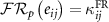 defines the Forman curvature FR of edge eij. In this case, equation (1) is particularly simple; the vertices and edges constitute the 0- and 1-cells and the closed loops in the graph constitute the 2-cells. In equation (1) there is no arbitrary restriction to the length of cycles that are admissible as bounding a 2-cell. The so-called ‘augmented’ FR is obtained by restricting these cycles to triangles. The geometrically more appropriate ‘enhanced’ FR
  [64] is obtained by truncating the expansion to cycles of maximum length 5.
Another very important property of CW complexes is that of quasi-convexity [22].
Definition 2. A CW-complex M is quasi-convex if, for each pair of  -cells α1 and α2 (viewed as topologically closed entities including their boundaries), if
  contains a p-cell β, then
  .
.
In the case of graphs, viewed as 2-complexes, this property reduces to the simple condition that any two cycles can share at most one edge (two edges share anyway always one link). Moreover, in view of the fact that only cycles of length up to 5 are relevant for local properties on the graph, we shall consider a reduced notion of quasi-convexity of graphs that imposes the condition of maximally one shared edge only for triangles, squares and pentagons. As we now show, this condition not only renders the computation of various combinatorial curvature measures tractable but it is a very physical condition representing a sort of ‘incompressibility’ of graphs; it was independently introduced in [28] and [29] where it was called ‘hard core condition’ or ‘condition of independent short cycles’.
For quasi-convex graphs, satisfying the independent short cycles condition, the prohibitive expression equation (1) reduces to the simple form

where ki denotes the degree of vertex i and  ,
,  and
and  denote the number of triangles, squares and pentagons supported on edge (ij), respectively [64]. This further simplifies for k-regular quasi-convex graphs,

These expressions show that, when degrees do not vary too much, combinatorial curvature is mainly determined by the number of local loops based on an edge, triangles contributing the most and pentagons the least.
2.2. Ollivier curvature
There are several variants of Ollivier combinatorial curvature (OR) [23–27]. Here we shall discuss only the simplest one, to be used to formulate GR on networks. Its basic idea is to reproduce in a discrete setting the geometric meaning of Ricci curvature.
While often introduced as a derivative expression of the metric, Ricci curvature on manifolds is a measure of how much infinitesimal spheres around a point contract (positive Ricci curvature) or expand (negative Ricci curvature) when they are parallel-transported along a geodesic with a given tangent vector at the point under consideration. The Ollivier curvature is simply a discrete version of the same measure. For two vertices i and j it compares the Wasserstein (or earth-mover) distance  between the two uniform probability measures
  on the spheres around i and j to the graph distance
  and is defined as

The Wasserstein distance between two probability measures µi and µj on the graph is defined as

where the infimum has to be taken over all couplings (or transference plans)  i.e. over all plans on how to transport a unit mass distributed according to µi on the unit sphere around i to the same mass distributed according to µj on the unit sphere around j,

While extremely intuitive from a geometric point of view, the OR seems even more cumbersome to compute in the generic case than the FR. This is why easier approximations have been developed [65–67]. Fortunately, however, these are not really necessary since the OR also simplifies substantially on quasi-convex graphs satisfying the independent short cycles condition [28]. In this case it takes the form [29],

where the subscript ‘+’ is defined as ![$[\alpha]_+ = \textrm{max} (0, \alpha)$](https://content.cld.iop.org/journals/2632-072X/6/4/042001/revision3/jpcomplexae29d3ieqn34.gif) and
and  ,
,  . For a k-regular quasi-convex graph this becomes

This shows that, when the degree distribution is rather peaked, also the OR of graphs is mostly determined by the number of short loops on an edge, where by short one means triangles, squares and pentagons. In this sense, the ‘geometry’ of graphs is a theory of loops. The quasi-convexity condition of independent short loops requires that such loops can touch along one edge but they cannot overlap more than this. It has thus a very physical interpretation as an incompressibility condition for loops (or graphs themselves), analogous to the hard-core condition for a gas of Bose particles [28]. As the hard-core condition prevents the infinite compressibility catastrophe of a Bose gas of particles, the corresponding hard-core requirement for loops also stabilizes a gas of loops on graphs, as we show below.
The incompressibility condition can be also formulated as an excluded sub-graph condition [29]. In figure 1 we list the subgraphs that must be absent for a graph to satisfy the independent short cycles condition and be thus quasi-convex.
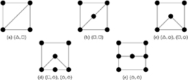
Figure 1. Excluded subgraph characterisation of the hard-core condition. Listed pairs for each subgraph give the types of short cycles sharing more than one edge.
Download figure:
Standard image High-resolution imageThis leads immediately to another interpretation of quasi-convexity. On a Riemannian manifold, the metric component  at a given point p defines a unique infinitesimal surface element on the tangent space in the plane spanned by the two directions i and j. The corresponding condition in the discrete graph setting requires that triangles, squares and pentagons, the fundamental local area elements, be uniquely defined by two edges. The excluded sub-graphs are exactly those for which this condition is not satisfied. In other words, quasi-convex graphs are those that satisfy the necessary condition for admitting a smooth continuum limit leading to a Riemannian manifold.
2.3. Comparison of the Forman and Ollivier curvatures
A general analytical comparison of the Forman and Ollivier curvatures is difficult because it is not simple to disentangle the contributions of the degrees and of the cycles. To make progress we will replace the degrees ki with their average value  , assuming that the degree distribution is sufficiently peaked. We then represent the so obtained OR curvature as a ‘mean field’ term, defined as the expression in equation (8) in which all brackets are simply summed up without taking into account the ‘+’ subscripts, plus a correction term. Essentially, the mean field term represents the dependence on the cycles alone, while the correction embodies deviations dependent on connectivity. This gives

where the correction to the mean field value  is given by

This shows that the properly enhanced Forman curvature coincides (up to an overall factor) with the mean field Ollivier Ricci curvature,

This result is remarkable, given that the two discrete curvature constructions have completely different origins. It is also an indication that the combinatorial dependence on the number of cycles is unique for any local discrete curvature measure.
The two curvatures become identical (up to an overall factor) when the quantity Iij defined by

satisfies  ,
,  . When
  , we fall in the first case of equation (10) and the correction term vanishes. When
  , the second case of equation (10) is realized and the correction term vanishes because it coincides with Iij. The condition
  ,
,  is realized for graphs with large connectivity and sparse cycles or, e.g. for all regular and semi-regular planar and hyperbolic tessellations involving triangles, squares and pentagons only. For these cases the appropriately enhanced Forman curvature and the Ollivier curvature coincide (up to a factor).
The case  is particularly interesting. This is the case for tilings of D-dimensional space, for which the skeleton degree
  , so that at each vertex one can choose to ‘move’ forward or backwards along D possible directions and where each of the edges supports exactly k − 2 elementary faces, triangles, squares or pentagons . In this case the OR becomes

This demonstrates that, in this geometric framework, triangles contribute positive curvature, squares contribute zero curvature, and pentagons contribute negative curvature. This is intuitively clear: triangles act as elementary units where ‘geodesics’ combinatorially converge, squares where they remain parallel, and pentagons where they diverge.
To further test the remarkable equivalence (11) one can generate a variety of random graphs with varying connectivity and edge density and compute both curvatures numerically to compare them [64]. For this simulation we consider Erdös–Rényi random graphs (see, e.g. [31]) using a varying link probability p in the range 0.01 to 0.1, after which we manually enforce the independent short-cycle condition by removing edges that violate it. For a fixed number N = 100 of vertices this generates graphs with an average degree  above the critical threshold for the emergence of a large connected subgraph. As p increases, the edge density of the graph increases, together with the density of short cycles. For each edge we compute Iij in (12), from which we build an average value: we expect that the two measures of curvature become closer and closer (up to the factor of
  ) when this average of Iij approaches zero.
In 2 we plot the average fractional difference between the two curvature measures,  over all edges in randomly generated graphs against the average value of Iij. For each link probability p we generate 10 graphs, to avoid the results being skewed by unusual graph configurations This simulation clearly shows that, here too, the two curvature measures differ when
  but, as Iij increases and approaches zero they converge to the same value.
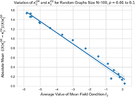
Figure 2. For N = 100 vertices we generate random Erdös–Rényi graphs, varying the link probability p. For a collection of 10 graphs for each value of p, we compute the average fractional difference between  and
and  , which we plot against the average of
  . The blue dots represent the raw simulation values, with the blue line representing the linear regression fit, shading to cover the 95% confidence interval for the regression.
Download figure:
Standard image High-resolution image3. Convergence of Ollivier curvature to Ricci curvature
To formulate GR on networks using a discrete curvature measure, it is essential to ensure that there is a regime in which this measure is mapped onto continuum Ricci curvature, which governs the large-scale Einstein equations. We will discuss two such limits. Here we show that Ollivier curvature converges to the continuum Ricci curvature as the network increasingly approximates a smooth manifold with a denser mesh [68]. Later we will show that even regular graphs, which are not dense, can define the 1-skeleton of a 2-cell complex which is a tessellation of hyperbolic space so that the geometric curvature is determined by the combinatorial one via the cycle structure at each vertex.
When working with purely combinatorial discretizations of curvature, associating a network with a manifold and its Ricci curvature requires assigning a distance scale to the graph’s edges. In the context of emergent geometry from a statistical network model, the simplest approach is to assume a fixed edge length, as we will discuss below. If the manifold is already given, a more natural choice is to weight each edge by the corresponding geodesic distance on the manifold. This allows one to meaningfully consider the limit of vanishing Ollivier balls centred on points of the manifold.
A notable example of networks defined over manifolds is the class of random geometric graphs (RGGs) [69] (for a review see [70]), which are constructed as follows. Given a manifold M, one sprinkles it with a Poisson point process of rate  , which determines the average density of points on the manifold. Two points on the manifold are connected if and only if their manifold distance does not exceed a threshold δn. The so obtained graph constitutes a random discretization of the manifold on a scale determined by n. This graph is the 1-skeleton of a Vietoris–Rips complex [71], whose topology was proven to converge to the manifold topology [72]. In [68] it was shown that also its geometry converges to the manifold geometry.
Consider a D-dimensional manifold M and a point x on it. Then pick a unit vector v at x and add a second point y at a distance δn from x along the geodesic in direction v. Finally let us consider a RGG on M with rate  and connection threshold δn dependent on n. The graph distances are weighted by the manifold distances: for every pair of vertices z and w on the graph, the graph distance
  is the sum of the manifold distances on the shortest graph path connecting z and w.
We want to compute the Ollivier curvature

as a function of n, where we consider uniform probability distributions µ on solid balls of radius δn, instead of spheres,

with  and a corresponding definition for the ball around y. The expression
  denotes the number of RGG vertices contained in the ball B, which, of course, depends on n. This is one the variants of the Ollivier curvature, which is the most appropriate for the convergence computation.
With these settings one can show that

if the ball radius shrinks to zero as,

The expectation value  is with respect to the RGG ensemble, in which
  is a random variable and Ric(v, v) denotes the continuum Ricci curvature at x in direction v. The above result is strong, in the sense that it does not only imply the convergence of the Ollivier curvature to the Ricci curvature of the underlying manifold, but also the concentration of the random
  around its expected value,

for any ε > 0. Since the expected average degree of the RGG behaves as

with  the ball in the manifold, the second condition in (17) requires that the graph be dense or sparse but not ultrasparse (or truly sparse), in which case
  . This shows that, for a sufficiently dense sampling of a Riemannian manifold M, a RRG G will approximate M as a metric space.
To conclude this section on discrete curvature, we would like to stress that the discussed Forman and Ollivier curvatures are not the only notions of discrete curvature that have been proposed. In particular we would like to mention the Bakry–Emery curvature [73] and the resistance curvature [74], although we will not discuss them in detail.
4. The emergence of hyperbolic manifolds
GR is a theory of dynamical manifolds governed by the Einstein–Hilbert action. At the classical level, the stationary points of this action, given by the Einstein equations, determine the space-time geometry for a specified matter distribution, or the vacuum geometry in the absence of matter. At the quantum level, one expects the Euclidean partition function, formally defined as a sum over all manifolds, to capture the quantum fluctuations around the classical solution. Yet, this is only well-defined when the manifold is discretized; otherwise, the Euclidean Einstein–Hilbert action is unbounded from below [8]. Euclidean dynamical triangulations (EDTs) still fail: they produce pathological manifolds with fractal dimensions. Introducing a preferred time foliation, as in causal dynamical triangulations, seems to cure the problem but, at least in the analytically tractable 2D case, it leads to relativistic invariance breaking at high energies, exactly as in Horava–Lifshitz gravity [75].
Here we will dispense altogether with the notion of a manifold. Using the Ollivier curvature as a combinatorial analogue of the Ricci curvature entering the Euclidean Einstein–Hilbert action we shall formulate a gravitational partition function as a sum over networks. The central question is whether well-behaved, fluctuating geometric manifolds can emerge spontaneously from such a formulation.
4.1. Cycle condensation
We consider thus a statistical mechanics model defined as a sum on quasi-convex 2D-regular graphs (QCG) with N vertices. The partition function is

where g is the dimensionless coupling and the Hamiltonian is defined as

where we denote by  the neighbour vertices j to vertex i in graph G, i.e. those connected to i by one edge (ij), 2D is the degree of the regular graph and
  is the Ollivier curvature (4) of edge (ij) (from now on we omit the superscript ‘OR’ since we will use only the Ollivier curvature). Note also that the constraints of quasi-convexity can alternatively be dynamically implemented by adding Kronecker-delta terms to the Hamiltonian [76].
It is important to stress that, contrary to the previously discussed case of RGGs, there is no embedding manifold assumed here. As we will show, however, at small coupling g the dominant graphs in the partition function (20) define themselves a manifold, specifically a surface, as 1-skeletons of 2-cell complexes. For this the constraint of quasi-convexity is a crucial ingredient; it is the free energy minimization under this constraint that leads to the emergence of manifolds.
Using the Ollivier curvature mean field plus correction representation (9) and (10), we can split the Hamiltonian into a global and a local contribution,
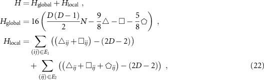
where  ,
,  and
and  are the total numbers of triangles, squares and pentagons on the graph and E1 and E2 are the ensembles of edges for which the respective summands are strictly positive.
The global term in (22) corresponds (up to a constant factor) to the Hamiltonian derived from the Forman curvature. It represents the Hamiltonian of a matrix model that depends solely on the total number of cycles in the graph. The energy is maximized for tree-like random regular graphs, which contain no cycles, and decreases as short cycles form. Among these, triangles contribute the most significant energy reduction, while pentagons contribute the least. The quasi-convexity condition, however, implies that a triangle can share an edge only with a pentagon, not with another triangle or a square, see figure 1. But it is energetically favourable to replace a triangle-pentagon couple with two squares, since  . Therefore, triangles and pentagons can survive only as isolated defects but are excluded for an homogenous ground state and we can henceforth neglect them. The global Hamiltonian is then minimized by increasing the number of squares. The local Hamiltonian, however penalizes edges for which the number of squares is higher than (
 ). The total expression (8) for the Ollivier curvature (with no triangles and pentagons) shows that these two effects cancel exactly when a configuration with
  squares per vertex and
  squares per edge is reached. Configurations with a higher number of squares (the maximum per edge is
  by regularity) are degenerate with this one. What happens is that, decreasing the coupling from the random configuration with sparse cycles, the number of squares at an edge increases until there are exactly
  squares based there. After this it pays energetically to increase the number of squares at another edge. This can continue until there are
  squares at each edge and
  globally. This is a hypercubic complex, which identifies D as the topological dimension of the ground state. For D = 2, this is a torus graph. The stability of the torus graph ground state has been discussed in detail and analysed numerically in [29]. To make numerical simulations less computationally intensive one can use bipartite graphs, for which there are no odd-length cycles. From here onward, we focus on the case D = 2 for which, as we now show, the ground state encodes the degrees of freedom of a 2D holographic screen, analogous to the framework proposed in Verlinde’s entropic gravity model [16, 17].
If only the global term is retained, the model undergoes a first-order phase transition in which the graph decomposes into isolated, weakly interacting hypercubic complexes [29, 77, 78]. If the full Hamiltonian is used, instead the model undergoes a continuous phase transition from a random graph phase to a geometric phase in which graphs become tessellations of smooth surfaces [28, 29, 34, 51, 52]. This phase transition is due to a condensation of square loops on the graph, while triangles and pentagons are suppressed and survive at best as isolated defects [29]. This is in agreement with a previous observation that the emergence of geometry in random networks is associated with clustering [79]. Random regular graphs are locally tree-like, with very sparse cycles, governed by a Poisson distribution with mean  for cycles of length k [80]. The order parameter for the transition is the density of squares
  , which increases from
  (for N = 160 in the example below) in the random phase to reach the maximum value 1 for a torus graph. It is shown in figure 3 as a function of
  .
.
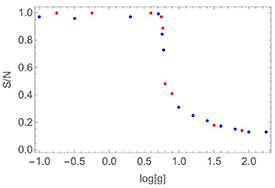
Figure 3. The order parameter  for the random-to-geometric phase transition for D = 2.
Download figure:
Standard image High-resolution imageThe red dots are obtained by starting with a torus graph and gradually increasing the coupling g; the blue dots, instead, correspond to decreasing the coupling from the random phase. Note the absence of hysteresis, as expected for a continuous phase transition. As could be expected, the Monte Carlo algorithm does not always manage to reach an exact ground state with  deep in the geometric phase when starting from a random graph configuration. Of course, several other diagnostics for a second order transition have been tested [29], with positive results.
Any finite graph has a genus, which is defined as the smallest genus of a surface on which it can be embedded as a 2-cell complex without any edge crossings [81]. Random graphs of N vertices can be embedded without edge crossings on a Riemann surface of genus N [82]. Therefore, decreasing the coupling from its critical value amounts to decreasing the genus of the emerged manifold until the ground state torus graph at g = 0 is reached. In figure 4 we show the example of a two-torus state at a small but finite value of g in the geometric phase.
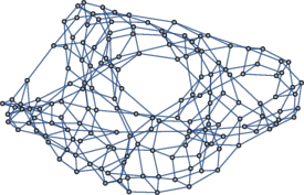
Figure 4. A two-torus at a small but finite value of the coupling g in the geometric phase.
Download figure:
Standard image High-resolution imageAs always in the case of continuous phase transitions, there in an emergent scale. This is the correlation length  , which vanishes in the ground state at g = 0 and diverges at the critical point. In the present case, let us consider the connected correlation function

between the number of squares  and
and  based on vertices i and j at fixed graph distance d, where
  denotes the variance (over the vertices) of the number of squares. The typical behaviour of this correlation in the geometric phase, as a function of d (at fixed g) is shown in figure 5.
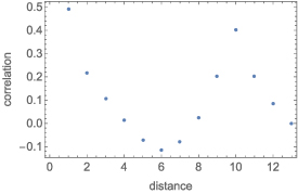
Figure 5. The typical behaviour of the connected correlation function between the numbers of squares at graph distance d in the geometric phase.
Download figure:
Standard image High-resolution imageAt extremely small distances the correlation is high since, given a square based at vertex i, there are always at least two vertices at distance 1 and one vertex at distance 2 that also support a square. At intermediate distances the correlation turns negative, because there is no correlation between squares on these distances but we are in the geometric phase, in which the average square number  is large. On these intermediate distances the graph behaves like a random graph. Correlations then suddenly pick up at the distance
  , before decaying again to zero on even larger distances. In this case, the approach to zero is not due to absence of correlations but, rather, to each vertex supporting the same number of squares
  . This is the geometric manifold phase on large scales. As usual, the correlation length
  separates the ordered phase (here the geometric phase), realized at large scales, from the remnants of the disordered phase (here the random phase) at small scales. The graphs in the geometric phase behave thus as geometric manifolds on distances larger than
  and as random graphs below this scale. To make contact with manifolds, we shall henceforth endow the links of the graph with a uniform length scale
  and identify the correlation length with the Planck length,
  . With this definition, the Planck length vanishes at g = 0 whereas at
  it equals the graph diameter.
Note that, strictly speaking, the continuous phase transition in this model of emergent geometry is fully characterized not just by the mean number of squares, but by the entire distribution of squares across the ensemble. In the random phase, this distribution is a Poisson distribution, with variance equal to its mean, as previously noted. In the geometric phase, the distribution becomes sharply peaked around its mean, approaching a delta function in the limit of zero coupling. Both phases are governed by a finite correlation length, which sets the scale for fluctuations and keeps the variance finite. At the critical point, however, the distribution becomes scale-free, and the variance diverges. This signals the emergence of ensemble fluctuations that include clusters of 4-cycles and random links on all length scales.
2D quantum gravity is often described as both trivial and pathological. It is considered trivial because it lacks local degrees of freedom, only the topological genus of the manifold plays a role. At the same time, it is deemed pathological because large quantum fluctuations cause the geometry to crumple into fractal structures with a Hausdorff dimension  . This behaviour is observed in both the continuum approach, such as Liouville theory, and in discrete formulations like matrix models or EDTs (see, e.g. [83, 84] for reviews). In contrast, the model studied here belongs to a different universality class. It features two distinct phases, one of which does not admit a manifold interpretation: this ensures the existence of local degrees of freedom at scales below the Planck length. Meanwhile, in the geometric phase, the quasi-convex graph structure gives rise to smooth manifolds with a Hausdorff dimension
  .
.
In this context, the Hausdorff dimension characterizes how the graph’s diameter  scales with the number N of vertices

This scaling relation captures the fractal nature of the emergent geometry in the large-scale limit. In the random phase, with logarithmic distance scaling, the Hausdorff dimension is infinite. Figure 6 shows the behaviour of  as a function of graph size N deep within the geometric phase. For graph sizes up to N = 1000, the Hausdorff dimension increases to values between 2.1 and 2.2. However, for significantly larger graphs, this growth is not only halted, it gradually reverses, with
  approaching 2 (the gap in data between N = 1000 and N = 2000 reflects the high computational cost: simulations at each value of N require months of CPU time). These findings support the conclusion that sufficiently large graphs in the geometric phase effectively approximate a smooth 2D manifold, unlike all previously studied models. This 2D manifold at large scales plays the role of a holographic screen analogous to what proposed in the framework of Verlinde’s model [16, 17], with some notable differences to be discussed below.
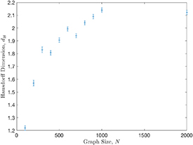
Figure 6. The Hausdorff dimension deep in the geometric phase as a function of size N.
Download figure:
Standard image High-resolution image4.2. Geometry from combinatorics
Regular graphs are ultrasparse and, as such, their combinatorial curvature is not sufficient to sample the continuum Ricci curvature on a manifold on which they are embedded, as we have shown above. There is, however, another way to map the combinatorial curvature onto a geometric curvature, as we now show.
We will henceforth consider the limit  , in which the emerging manifolds are the covering spaces of genus g Riemann surfaces, i.e. infinite surfaces of negative curvature, so-called Cartan–Hadamard surfaces (for a review see [85, 86]). To simplify things, we will initially forget about the small scale randomness and, also, we will consider first configurations in which each vertex supports the same number
  of squares. These correspond to a quantized constant negative curvature, as we now show.
In the geometric phase, graphs become the 1-skeleton of a 2-cell embedding, for which the graph cycles are homeomorphic to open disks on a surface. The 2-cell embedding is called a ‘map’. A combinatorial map can be geometrized by assigning the same fixed geodesic length  to each edge so that it becomes a tessellation of the surface, in which the combinatorial cycles become regular polygonal faces of the tessellation [87–89].
Each edge of the map supports exactly two regular polygons, each vertex supports exactly four polygons. Let ki,  , be the number of edges of the 4 polygons surrounding a vertex and let us call the vector
  the vertex type. For simplicity, we shall consider homogeneous maps, for which the edge type is the same for all vertices, so that the geometrization gives rise to semi-regular tessellations. For such maps, the tessellated surface is a constant curvature surface given by the angle sum parameter

If α < 2 the surface is spherical, i.e. of positive constant curvature, if α = 2 it is the flat Euclidean plane and, finally, if α > 2 it is hyperbolic, i.e. of negative constant curvature [87–89].
For every hyperbolic tessellation there is exactly one geodesic length so that the sum of interior angles at each vertex sums exactly to 2π. To see this, let us use the cosine rule for a hyperbolic n-gon,

to write the total interior angle at a vertex of a tessellation as

where R is the radius of curvature of the Poincaré disk on which the tessellation is constructed. First of all let us note that this is a monotonically decreasing function of  . Second, for
  the total interior angle vanishes. In the opposite limit
  , the solution of (27) requires α = 2, i.e. the geometry becomes Euclidean. Therefore, given a specific semi-regular hyperbolic tessellation, there is exactly one possible parameter
  that solves (27). If the length unit
  is held fixed, the hyperbolic radius R of the Poincaré disk varies and, with it, the curvature
  . Otherwise, we can describe varying curvature at a fixed radius by letting the length unit
  change. The tessellation realized by the graph minimizing the free energy at every coupling g determines the value of the curvature K(g) in units of
  .
.
The geometric phase is realized by the condensation of squares and corresponds, thus to vertex types with at least one  and all other
  or
or  for all vertices. At each coupling, one of the four possible vertex types of the semi-regular tessellation, with one, two, three or four squares will characterize the minimum of the free energy, the remaining larger cycles determined by the detailed balance between the combinatorial energy and entropy. When the coupling is decreased from the critical value, the number of squares corresponding to the free-energy minimum will typically increase. For sufficiently large steps, one of the ki decreases from a higher value to 4. In order to maintain the total interior angle sum as 2π, as in (27), the quantity
  has to decrease, which means the absolute value of the curvature of the tessellated surface typically decreases, until it vanishes for four squares around each vertex. In figure 7. we show one example of such a tessellation with three squares and one hexagon per vertex, corresponding to a constant negative-curvature surface at a small but non-zero value of the coupling g.
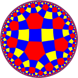
Figure 7. The 2D tessellation geometrizing the three-square-per-vertex infinite graph via its 1-skeleton.
Download figure:
Standard image High-resolution imageNote that one cannot take the length scale  to zero without the curvature also vanishing. In the infrared, the model is pushed to the completely ordered zero-coupling state corresponding to a flat geometry. At small, but non-vanishing coupling g the surfaces emerging from the network gravity model are characterized by two connected scales, a fundamental length scale
  and a radius of curvature R. At zero coupling the former vanishes and the latter diverges, at the critical coupling the former diverges and the latter vanishes.
Via this construction, the purely combinatorial Ollivier curvature is mapped to geometric curvature. The value of this curvature is determined by the statistical balance between the combinatorial energy dependent only on square cycles and the entropy representing the possible choices of residual larger cycles. Of course, in the general case, the tessellation will not be semi-regular, corresponding to surfaces with possibly varying negative curvature, so-called Cartan–Hadamard surfaces [85, 86]. And finally, on scales smaller than  , there are random microscopic degrees of freedom.
5. Dynamics
Until now we have dealt with static configurations minimizing the free energy at a given coupling g. To analyse the dynamics, i.e. the fluctuations around these free energy minima, we need to introduce a universal Newtonian time t. Given an edge configuration  , a transition to a modified edge configuration
  takes place with a probability

Of course, the transition has to be kinematically allowed, i.e. respect the regularity of the network and quasi-convexity and therefore must involve at least two edges. One such local, elementary fluctuation preserving regularity is the ‘neighbourhood swap’, shown in figure 8. On a square lattice, e.g. this move replaces three squares with two pentagons. It represents thus a local curvature fluctuation which, by a simple combination of four-edge moves, can propagate on the lattice.
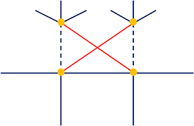
Figure 8. The regularity-preserving neighbourhood swap move.
Download figure:
Standard image High-resolution imageLet us now consider a cluster of random phase at a small but non-vanishing value of g. The boundary of such a cluster is made by all vertices which support at least one non-accidental square, meaning that at least one of its neighbours supports more than one square. In general there are two types of fluctuations, one that changes shape and size of the clusters (akin to Glauber fluctuations in the Ising model) and one that corresponds to translations of the clusters at fixed order parameter (akin to Kawasaki fluctuations in the Ising model). Indeed, the energy of a cluster depends exclusively on the number n of vertices in its bulk (supporting no short cycles) and on its boundary configuration. Therefore, a configuration replicating exactly the same cluster at a different location on the tessellated surface has exactly the same energy. A collective move implying a translation of the cluster costs no energy. Because of detailed balance in the equilibrium state, such zero modes will perform diffusive Brownian motion. Of course, it is an open question, beyond the scope of this review, how the collective translation can occur in terms of elementary edge moves. In any case the average velocity v of this collective Brownian motion is limited by above by a velocity c determined by the length  and the inverse number of elementary moves per unit time, which are the two sole fundamental units in the model.
5.1. Hyperbolic holography
To proceed we shall consider a large-scale hydrodynamic approach consisting of point defects in Brownian motion on a constant negative-curvature surface. It turns out that curvature has a profound effect on Brownian motion, with momentous consequences: in the case of negative curvature it is anomalous and becomes asymptotically ballistic.
Let us consider a constant negative curvature surface as the upper sheet of a two-sheeted hyperboloid embedded in 3D Minkwoski space with metric  as
as

The metric is d , with
  with
with  and
and  the curvature.
For  (with
(with  the diffusion coefficient), the Brownian motion b(t) on such a manifold can be expressed as

where  is the Brownian bridge, the Brownian motion b(t) constrained to come back to the origin x = o for t = T. The quantity
  is called the infinite Brownian loop [50]. If
  for
for  , as in the typical case, the infinite Brownian loop is the Brownian motion itself. Not so, however, if the Brownian motion is ballistic,
  for
for  . This is exactly the case in negative curvature.
Brownian motion on a negative curvature surface decomposes in two independent radial and angular Brownian motions  [44–46] (for a review see [47–49]). For
  , the angular component converges to a limiting angle
  , while the radial component becomes ballistic,

where  is the inertial velocity of the defect and
  is the diffusion coefficient, which depends on its size. Asymptotically, the manifold coordinate z is dynamically soldered to the absolute time and Brownian motion acquires a deterministic component describing inertia in negative curvature. The exponential volume growth due to negative curvature creates a surface of last scattering: after the typical time scale
  background fluctuations decouple and the defect moves on radially with the velocity v it had after the last scattering [51, 52].
Let us focus first on this deterministic component. The asymptotic inertial trajectories (31) at different angles  diverge because the negative curvature implies an exponential volume growth when z increases. Up to an exponentially small correction, these trajectories are the same as the comoving geodesics on a 2D Lorentzian manifold of positive curvature
  , realized by the embedding

with the metric

This is 2D de Sitter space-time (for a review see [90]), in which comoving geodesics diverge dynamically because of the Hubble expansion with parameter J (see [90]). Asymptotically, inertially diffusing observers in Riemannian negative curvature are equivalent, up to an exponentially small correction, to comoving observers in Lorentzian positive curvature [51, 52]. One can use both descriptions; however, with positive curvature, the universal time t becomes the coordinate time of a Lorentzian manifold. This is a form of Wick equivalence arising between the two signs of curvature.
In general, diffusion processes probe the intrinsic geometry of a manifold via the return probability kernel  . The quantity
  is called the spectral dimension and measures the effective number of dimensions available to a random walker on the scale reached by time t, essentially on small scales for t → 0 and on very large scales for
  . The spectral dimension is of paramount importance, since it is the dimension perceived by local physical processes.
Unfortunately, this does not work as usual in the present framework, because of the dominant ballistic component of Brownian motion, which is much too fast to probe the local geometry. The Laplacian on a constant negative curvature manifold has a spectral gap

representing the bottom of the spectrum of the positive operator  , which is associated with asymptotic ballistic behaviour. As a consequence, the return probabilities K(t) are dominated by an exponential behaviour at large t [55, 91],

which gives a spectral dimension linearly diverging in time.
The large-scale local geometry, however, is probed by the sub-dominant random component of Brownian motion, the infinite Brownian loop [50], whose return probabilities are given by (35) without the dominant exponential factor and give, therefore the spectral dimension function

The spectral dimension on scales smaller than  is D and coincides with the topological dimension (D = 2 in our case), while the large-scale spectral dimension at distances larger than
  becomes 3, independently of D. In the mathematical literature this is called the ‘pseudo-dimension’, or ‘dimension at infinity’ of the constant negative curvature manifold [50]. The large-scale spectral dimension 3 is not confined to a constant negative curvature manifold though, but is valid for any manifold with strictly non-positive curvature and is a consequence of the central limit theorem in negative curvature [54]. This scale-dependent spectral dimension reproduces similar results in causal dynamical triangulations [8, 9] and Horava–Lifshitz gravity [3], with the difference that, here, there is a fundamental scale separating the two regimes.
When we take into account the sub-dominant random component of negative-curvature Brownian motion two things happen: first, the universal time t does not coincide anymore with one coordinate, secondly, an additional space dimension emerges spontaneously, a phenomenon we shall denote by hyperbolic holography. Let us consider the radial heat kernel  on negative curvature, for distances
  , such that the angular distribution is uniform,

where the radial Laplacian is given by

and we have introduced, for simplicity of presentation, dimensionless quantities  and
and  . The kernel
  admits the representation [50]

where f0 is the symmetric ground state of the Laplacian corresponding to the spectral gap [55]

for  . The residual kernel
  describes the infinite Brownian loop random process, obtained by subtracting out the dominant ballistic component. It encodes the random dynamics of the defects as seen by an observer comoving with the inertial flow and satisfies the modified heat equation

Using (40) and  , this equation becomes

where  is the radial Laplacian in a 3D Euclidean space. Therefore

where we have reintroduced the original variables. This is the isotropic heat kernel on a 3D Euclidean manifold with distance norm z ‘inherited’ from the hyperbolic distance on the holographic screen [50]. In the Riemannian negative-curvature picture, the observer is comoving with the inertial flow of ballistic diffusion; in the Lorentzian positive-curvature picture, the observer is comoving with the Hubble flow on the holographic screen. If this Lorentzian picture is used for the dominant flow, the comoving random process must be treated as time-symmetric in the forward and backward directions, which gives immediately the Schrödinger evolution [92]

where we have used the previously introduced time  measured in seconds. This is the 3D Schrödinger propagator for a particle of mass
  , velocity
  and therefore Compton wavelength
  . This is the definition of the ratio
  , more about this in the next section. At large scales, the local random process, as seen by geodesically free-falling observers on a de Sitter holographic screen, is quantum mechanics in an effective 3D Euclidean space with distances given by the hyperbolic distance on the holographic screen.
Quantum mechanics arises because the physical evolution parameter t, identified with coordinate time at large scales, must be treated as Lorentzian, when using the comoving interpretation of the dominant inertial flow. When constructing the Lorentz-invariant, but non-reparametrization-invariant action in terms of t, the fluctuations at small scales are sampled with the phase factor exp(iS). The Wick rotation is automatically enforced by the dominant comoving flow. The holographic promotion of the screen distance to an effective distance in a 3D Euclidean space immediately then implies quantum behaviour in this emergent space. The appearance of quantum behaviour, therefore goes hand-in-hand with the Lorentzian signature of space-time and vanishes with it below a scale fixed by the radius of curvature of the holographic screen.
6. Emergent large-scale physics
6.1. Matter, the Einstein equations and the cosmological constant
In the previous section we have derived the emergence of an effective 3D Euclidean space ‘seen’ at large distances by quantum particles in a comoving frame of a de Sitter holographic screen. In this section we consider the holographic screen and the emergent space as embedded in a common large-scale bulk Universe manifold. To this end let us consider the isometry groups of the two components. The isometry group of a constant-curvature 2D holographic screen is  , where the + indicates the orthochronous subgroup if the curvature is negative, in which case an arrow of time is built in. The isometry group of the emergent 3D Euclidean space is SO(3). The construction of an embedding Universe must be such that these two isometry groups share a common SO(2), corresponding to the angular variable of the holographic screen, and that 3D spatial distances scale with the same exponential factor as on the holographic screen, see (43). These requirements are satisfied by an isometry group SO(1,4) [93, 94], which corresponds, in the effective Lorentzian picture, to a (1+3)-dimensional de Sitter spacetime. The effective curvature experienced in this ‘bulk’ de Sitter Universe need not coincide with that of the holographic screen, since rescalings of time and of the speed of light can be absorbed into the definition of the de Sitter radius. Consequently, the non-relativistic quantum mechanics (44) can be ‘lifted’ to relativistic quantum field theory in an effective bulk de Sitter space.
Let us now consider a random phase bubble embedded in a constant curvature graph at low, but finite coupling. The interior vertices of the bubble support no squares (apart accidental ones). The boundary vertices of the bubble also support typically less squares than the surrounding graph, since at least one edge has to connect them to the random graph inside. Moreover, the remaining long cycles based on edges of the boundary vertices are much longer than in the surrounding geometric phase, since they have to cycle along many vertices in the interior random graph before coming back. These energy and entropy effects conspire to generate the higher free energy of the random phase bubble with respect to the geometric surrounding. But also, each vertex on the boundary has a lower curvature since less squares and longer cycles imply a larger excess angle at the vertex, so that the curvature is more negative than in the geometric phase, as explained above. Since the number of boundary vertices depends on the bubble size, this lower negative curvature is associated with the higher free energy, but this relation is statistical in nature since many microstates of slightly different curvature, due to long cycles entropy, characterize the ensemble with a given free energy. The ensemble equation is thus

in units where the free energy F is measured in Joule with respect to the surrounding geometric matrix with curvature  .
.  is Newton’s gravitational constant and n(g) is a numerical factor depending on the original coupling g.
In the Lorentzian picture the curvature changes sign. Let us consider also the large-scale continuum approximation in the bulk Universe, where the random bubble becomes a point-like excitation at rest in the comoving frame. In this case we must consider density distributions by dividing both sides by  . This gives

where f is the free energy density, measured here with respect to the bulk curvature  , and we have used the standard notation R(x) for the continuum Ricci curvature in (1+3) dimensions. Since both the free energy and the curvature of these random phase defects are higher than the surrounding manifold on which they live it is natural to identify them with matter particles, although they are made of the same microscopic degrees of freedom as the surrounding space.
In a generic frame, the energy–momentum tensor of a dust of such particles moving along geodesics must be defined by a local (maximum two derivatives), symmetric geometric tensor which is covariantly conserved and has equation (46) as its trace. The unique such geometric tensor is the Einstein tensor augmented by a cosmological constant term [95], which gives

These are Einstein’s equations of GR (with a cosmological term), with the difference that Tµν must be interpreted as a (density) thermodynamic potential and the equations hold as statistical ensemble averages. In this model these are not dynamical equations but, rather, macroscopic constitutive equations of matter as defined by the microscopic network degrees of freedom.
Matter, in this model is simply the random phase of the microscopic network. Matter particles have two sizes: a gravitational size  where their associated excess curvature is concentrated and a quantum size, the Compton wavelength, set by the screen radius of curvature. In the present model, at large scales, it is ‘geometry that defines matter’, not the other way around, as usual.
In this model, there is an obvious possible solution to the cosmological constant problem (for a review see, e.g. [96]): the zero-point energy of quantum fields curves only the holographic screen, only matter and geometric fluctuations curve the bulk Universe. Note that the free energy of the model is, by construction, a very small positive quantity for a Universe empty of matter, with only geometric fluctuations on the scale of the cutoff  .
.
6.2. Black holes, Hawking radiation and absence of information paradox
As discussed above, matter is modelled as the random phase of the network. At finite coupling  , matter particles are identified with the residual bubbles of random phase embedded in the dominant geometric matrix, representing the space manifold. Their typical size, the Planck scale, is stabilized by the balance between energy and entropy at the given coupling.
These bubbles diffuse due to the underlying network fluctuations and, in the continuum approximation at large scales, their dominant dynamics in the Lorentzian picture is described by a thermodynamic energy momentum tensor defined by the Einstein equations statistically in terms of network curvature. As a consequence, matter particles will tend to aggregate under the influence of gravitational forces. This is balanced by repulsive effects, among which quantum ones, such as the uncertainty relation and statistical pressure for fermions, but also thermal and radiation pressure and other interactions. However, if many particles do manage to approach each other on distances of the Planck length order, their random networks can merge to form a larger bubble of random network. And if the resulting bubble becomes larger than the radius of curvature scale, we have a single macroscopic 3D quantum object. This is a black hole.
Actually the hole is not really black. Let us consider the typical times τG and τR necessary for information to traverse a geometric and a random region of the same size L. In the geometric phase  , where
  is the number of network vertices making up the region and D = 2 on the screen or D = 3 in the emergent space. In the random phase, instead,
  . To achieve the same dimension L, we must choose
 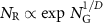 . Therefore, to cover the same distance L in the random phase, information must take exponentially more steps than in the geometric phase. If every edge is traversed with the same speed, this entails that the time needed to traverse a region of size L of random phase is exponentially larger than the time it takes for the same distance on the geometric matrix,

The random phase acts as a retardant medium for information propagation due to the disorder associated with the lack of a coherent geometric matrix. From the point of view of an observer in the geometric matrix, clocks in the random phase tick exponentially slower. Albeit exponentially large, however, the time delay associated with traversing a large random phase bubble is still finite. After a very long time, information will come out of the random phase region; only in the continuum limit  and
and  with
with  finite does the hole develop an event horizon and become really black, since information has to make infinite steps to come out. However, in this limit no random phase survives. True black holes are thus only a continuum idealization which does not exist at finite Universe curvature.
Note that k-regular ( ) random graphs are excellent expanders: the number of vertices within a ball of radius r scales like the number of vertices at distance r, where r denotes the level of hops along the tree leaves. Asymptotically for
  , the ‘surface to volume ratio’ of the graph is
  , 2/3 for 4-regular graphs. This means that there is essentially no distinction between volume and surface since 2/3 of the volume is taken up by the boundary surface. Since the boundary is well-defined from the embedding in the geometric matrix, the black hole is essentially only a very thin surface layer. All the vertices of the random bubble are concentrated there. This is the origin of the holographic principle: the number of degrees of freedom of a black hole scales with the area of the (would be) event horizon. The holographic principle for black holes is thus an immediate consequence of the expander property of regular random graphs.
The same expander property is shared by hyperbolic space. Since the geometric matrix of the screen is a negative-curvature surface, it is natural to visualize the black hole also as embedded in a 2D hyperbolic space, for which the surface to volume ratio is  , the inverse of the radius of curvature. To do so we must assign to the graph edges a fixed length unit
  and then equate
  to
to  , which gives a curvature radius
  . Finally, if we want to compare this to the surrounding geometric matrix, we must rewrite the logarithmic distances in this hyperbolic bubble as
  where
where  is the number of vertices in it and
  . For large bubbles, the ‘inside’ effective edge length is exponentially smaller than the corresponding one in the geometric phase outside, which implies that the black hole can be seen as a hyperbolic bubble of exponentially large curvature with all degrees of freedom on the surface.
The expander property of the random phase implies that black holes are essentially large circles of radius R on the holographic screen. Their free energy, measured in Joule, can thus be expressed as

where u and s are numerical constants determining internal energy and entropy, respectively. We identify the internal energy as the black hole mass (times velocity squared),

which, for u = 1 is the Schwarzschild value. Seen from afar, these black holes appear as 2D surfaces, since their scale is much larger than the screen radius of curvature. If we want to interpret correspondingly the entropy as distributed on this surface, we must multiply it by a factor  and divide simultaneously the dimensionless ‘temperature’ g by the same factor. This gives the physical temperature and entropy seen in the bulk,

For g = 1 and  these are the Hawking temperature [97] and the Bekenstein entropy [98]. The exact values of these numerical factors depend, of course, on the microscopic statistical mechanics of the underlying network. However, the qualitative facts that black holes are characterized by an entropy proportional to their perceived horizon area and by a temperature inversely proportional to their mass are natural, but non-trivial predictions of the network model.
Bubbles of random phase much larger than the Planck length are not stable since they are not minima of the network free energy. When such a large bubble forms it will stabilize by shrinking to its equilibrium size by emitting both energy and entropy. This is a simple explanation of the Hawking radiation of black holes. They are simply statistically unstable and they emit energy and entropy to return to their equilibrium size.
Finally, since information is always stored in the fundamental network, there is no information paradox. When information falls into the black hole it is simply stored provisionally in another network phase and then released back when the hole stabilizes to its equilibrium size.
6.3. Dark matter
Dark matter is one of the major puzzles of contemporary cosmology (for a review see, e.g. [99]). The mass-energy of the Universe is made only by 5% of ordinary baryonic matter, the remainder being 27% dark matter, an unknown form of matter interacting with ordinary matter only through gravity and 68% dark energy, attributed typically to the cosmological constant discussed above.
There are two possible avenues to tackle the dark matter problem. One is to posit a new type of particle, with essentially only gravitational interactions, which is the mainstream belief today, the other is to posit a modification of classical GR. In [17, 35], however, it was proposed that dark matter is a macroscopic manifestation of quantum gravity. We now focus on how dark matter naturally fits in the present model.
We have shown that the holographic graph can have two phases, a random phase, identified with ordinary matter, in which there are no short loops and a geometric phase, representing space, in which each vertex i can exist in four possible states, corresponding to the number  of squares surrounding it. The number
  determines the quantized curvature at this vertex as shown above. Until now we have focused on uniform curvature configurations in which all vertices in the geometric phase have the same number
  of squares and we have shown that this curvature is inherited in the emergent (1+3)-dimensional space-time.
What about inhomogeneous space configurations with different values of  ? Imagine, in particular that the coupling g decreases from the critical coupling
  so that the Universe emerges from an all-random state at an extremely high curvature
  , representing the big bang. As always when lowering the coupling in continuous phase transitions, there typically survive domains of higher free energy. These are metastable states, which, depending on their free energy difference to the minimum and the barrier in between, may be extremely long-lived. These states are called allotropes and the most famous example are the two states of carbon, graphite, the free energy minimum and diamond the higher free energy allotrope (for a review see [100]).
In the present case, we can have metastable domains characterized by a higher number  than the prevailing configuration
  and therefore having a larger free energy than the space around them at a given g. Because of this higher free energy they have also a higher curvature (in the Lorentzian picture) and interact gravitationally. But they are neither empty space nor ordinary matter. These domains are natural candidates to represent dark matter in the Universe. Dark matter, in this model, appears like crystal allotropy in the network fabric of space-time. An example is shown in figure 9.
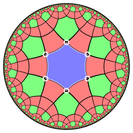
Figure 9. An allotropy region (blue) with vertices surrounded by two squares within an hyperbolic tessellation with all vertices surrounded by three squares. The hyperbolic tessellation represents space of a given uniform curvature; the blue allotropy region represents a region of dark matter, with a higher absolute curvature and free energy. For simplicity of presentation we are showing here only the smallest example of such a region. Created by Eryk Kopczyński using RogueViz [101].
Download figure:
Standard image High-resolution imageOf course, for couplings g midway between values favouring two different number of squares as the free energy minima, small domains of lower absolute curvature can form before the whole space-time transitions to this configuration. These would correspond to antigravity domains within a uniform metastable Universe.
Data availability statement
No new data were created or analysed in this study.