Abstract
Photoemission orbital tomography provides direct access from laboratory measurements to the real-space molecular orbitals of well-ordered organic semiconductor layers. Specifically, the application of phase retrieval algorithms to photon-energy- and angle-resolved photoemission data enables the direct reconstruction of full 3D molecular orbitals without the need for simulations using density functional theory or the like. However, until now this procedure has remained challenging due to the need for densely-sampled, well-calibrated 3D photoemission patterns. Here, we present an iterative projection algorithm that completely eliminates this challenge: for the benchmark case of the pentacene frontier orbitals, we demonstrate the reconstruction of the full orbital based on a dataset containing only four simulated photoemission momentum measurements. We discuss the algorithm performance, sampling requirements with respect to the photon energy, optimal measurement strategies, and the accuracy of orbital images that can be achieved.
Original content from this work may be used under the terms of the Creative Commons Attribution 4.0 license. Any further distribution of this work must maintain attribution to the author(s) and the title of the work, journal citation and DOI.
1. Introduction
Image reconstruction based upon sparse Fourier space measurements is a problem that recurs in a wide range of imaging modalities, with well known examples being x-ray computed tomography [1, 2] and magnetic resonance imaging [3]. In fields such as coherent diffractive imaging [4, 5] and photoemission orbital tomography [6], the challenge of image reconstruction is further increased due to the inherently incomplete measurement data: whereas image reconstruction requires the complex-valued field to be known, only the amplitude can be measured. For the latter two, iterative image reconstruction methods nowadays enable high-resolution imaging with only limited prior information [7, 8], but these methods still require strongly oversampled data to achieve this. In many cases, particularly for photoemission orbital tomography which concerns itself with the quantum-mechanical electronic orbitals of molecules, the object of interest is intrinsically sparse, and this can be efficiently exploited using the ideas of compressive sensing surveyed in [9].
Photoemission orbital tomography (POT) is well established as a probe of the electronic structure of thin molecular films. Until recently, the conventional approach of this method to achieve information on the molecular orbitals would be the comparison of angle-resolved photoemission spectroscopy (ARPES) data to simulations generated using density functional theory (DFT) [10–13]. Iterative phase retrieval, however, allows one to reconstruct the orbitals directly from the measurements [6, 8, 14], and this is independent of DFT or similar calculations (see figure 1). While spatially resolved access to the electron density of molecular orbitals can also be achieved, e.g. by scanning tunneling microscopy [15, 16], the unique nature of POT provides several advantages to probe the molecular orbitals at high resolution. Most notably, together with gas-phase molecular orbital tomography [17, 18], POT using photon-energy-dependent ARPES measurements is uniquely suited to image the full three-dimensional (3D) molecular orbitals, and POT remains so far the only technique that can do so for larger, nanometer-scale molecules [19, 20]. Such 3D-POT is highly promising, as the combination with time-resolved photoemission orbital tomography [21–24] will access spatio-temporal properties of the dynamic electronic wavefunction that are so far inaccessible by experimental means. Additionally, 3D-POT promises a crucial insight at hybrid interfaces, where strong modifications of the electronic structure are known to occur [25, 26].
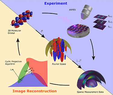
Figure 1. Photoemission orbital tomography provides access to the three dimensional structure of molecular orbitals (top left) by combining photon-energy- and angle-resolved photoemission spectroscopy (ARPES) with image reconstruction methods. Here, the photoelectron distribution of an ordered molecular layer measured at different photon energies  (top right) corresponds to the amplitude squared of hemispherical cuts through the three dimensional Fourier space (center). Based on the sparsely sampled Fourier space (bottom right) the initial molecular orbital can be reconstructed using a cyclic projection algorithm (bottom left) that incorporates constraints such as sparsity, support and symmetry in real-space and the measurement data and a low-pass filter in momentum space.
Download figure:
Standard image High-resolution imageHowever, despite the rapid development of powerful multi-dimensional photoelectron detection schemes [27–29], their application for 3D-POT has remained limited for a number of reasons: First and foremost, the application of phase retrieval algorithms requires a high-resolution 3D momentum distribution, implying the time-costly measurement of an ARPES dataset with a large number of photon energies, where, furthermore, the photon flux must be accurately calibrated. Moreover, the plane-wave model of photoemission, upon which phase retrieval methods are based, is only an approximation with respect to the overall photon-energy dependence of the photoelectron intensity [30, 31]. In this article, we deal with these challenges using a fundamentally new approach for 3D-POT: by implementing ideas from sparse optimization [32], we perform an image reconstruction on a pixelized object that is defined by the combination of several qualitative constraints in addition to sparsity constraints.
In section 2, we review the fundamentals of 3D-POT, and identify the challenges that must be solved to facilitate an efficient access to the 3D molecular orbital. We translate this theoretical description to an image reconstruction problem in section 3, and explain how this non-convex problem can be solved by a cyclic projection algorithm with several qualitative constraints. In particular, we propose to reconstruct the full molecular orbital using a combination of sparsity, a loose finite support and, when available, symmetry of the real-space molecular orbital. The orbital reconstruction from simulated data for an isolated pentacene molecule is demonstrated in section 4. After establishing the convergence behavior of cyclic projections in this setting, we focus on two questions: first, how many photon energies must be measured for accurate orbital reconstruction, and second, we investigate how experimental noise such as counting statistics and inaccurately estimated light intensity calibration affect the reconstruction.
2. Theory of 3D photoemission orbital tomography
In image-reconstruction photoemission orbital tomography, we consider an ordered molecular layer in which the unit cell consists of a single molecule (e.g. a monolayer of pentacene on Ag(110)), and use the plane-wave model of photoemission to calculate the ARPES signal. In this case, for a given molecular orbital ψ the ARPES signal I for the photoelectron momentum  can be expressed as

Here  is the vector potential of the ionizing radiation,
  , the Fourier transform of the molecular orbital, and
  denotes the absolute value of
  at the point
  in momentum space. The Dirac δ function stems from Fermi’s golden rule and ensures energy conservation, taking into account the ionization potential
  of the molecular orbital, the final state kinetic energy
  and the photon energy
  .
.
Note that  is proportional to the magnitude squared of the momentum
  ; hence, a single ARPES measurement provides the amplitude of the orbital’s momentum distribution along a hemispherical shell with a radius that depends directly on the photon energy
  . In order to probe the full 3D momentum distribution
  of the molecular orbital, it is therefore necessary to measure ARPES patterns for multiple photon energies. This naturally leads to a question that is central to the work that we present here: How many photon energies are required to yield a reliable orbital reconstruction from ARPES momentum maps? Before it is possible to address this question, however, first a strategy must be established that enables the reconstruction of a 3D molecular orbital from a sufficiently large dataset.
A reconstruction strategy for 3D photoemission orbital tomography (3D-POT) must solve two problems: 1) Starting with an ARPES dataset that only contains discrete cuts through the 3D photoelectron momentum distribution, the complete 3D photoelectron momentum distribution must be determined, and 2) the phase distribution corresponding to the measured amplitudes must be resolved. Up until now, these steps have been performed sequentially: first, the 3D momentum distribution is completed using an interpolation algorithm [19]. Subsequently, the full 3D momentum distribution can then be used as input of an iterative phase retrieval algorithm, which is the standard approach to determine the phase pattern in 2D orbital imaging as well. The interpolation step has significant implications: here, it is (implicitly) assumed that the momentum distribution is of a shape, or regularity, that can be interpolated and furthermore that it is properly sampled. Such Fourier-space interpolation, however, is prone to errors, particularly when also the intensity-only nature of the measurement is taken in account. Consider for example a zero crossing in the momentum distribution  . Here, intensity measurements at opposite sides will both yield non-zero intensity, and interpolation of this data will lead to the false conclusion that the intensity in-between must also be non-zero. The size of the error introduced here decreases as the sampling density increases, meaning that an accurate reconstruction of 3D molecular orbitals through this sequential approach relies on large datasets in which many photon energies have been measured.
In order to reduce the number of ARPES measurements needed and, more importantly, to prevent errors arising from the interpolation procedure, it is thus clear that a completely different reconstruction strategy must be developed. To that end, we now consider the phase retrieval algorithms that are already commonly used in orbital reconstruction POT. Generally, these are mathematical optimization algorithms that aim to find a solution that best satisfies a set of constraints. In POT, the solution corresponds to the image of a molecular orbital, while the set of constraints consists of the ARPES measurements and the prior knowledge about the molecular orbital. These algorithms are commonly referred to as phase retrieval algorithms because they reconstruct the phase that is lost upon the measurement, but the recovered information can include intensity as well as phase. For example, phase retrieval algorithms in coherent diffractive imaging are already routinely used to also recover the intensity in parts of the diffraction pattern that cannot be measured [33, 34]. As such, a promising approach to reconstruct 3D molecular orbitals from a discrete set of ARPES measurements is to generalize the already-necessary phase retrieval algorithms to 3D reconstruction algorithms. In this article, we build upon the sparsity-driven phase retrieval algorithm for orbital imaging [8] to develop a 3D-POT reconstruction algorithm. In particular, using the compact and voxel-sparse shape of the molecular orbital as a real-space constraint, we present an algorithm that efficiently and accurately interpolates the momentum distribution based upon ARPES measurements at just a few photon energies.
3. Basic approach
In this section, we will lay the foundation of an image reconstruction method based on the description of the 3D-POT measurement in (1). Readers who are instead interested in the results of the 3D orbital image reconstruction algorithm are encouraged to proceed to section 4. Now, we will first consider the properties of the experimental data and define the mathematical image reconstruction problem that follows from this description. To solve this problem, we will then define a multi-constraint feasibility model, where in addition to the measurement data we implement (i) a low-pass filter in momentum space, (ii) sparsity of the voxelized real-space molecular orbital, (iii) symmetry and (iv) a loose support of the real space molecular orbital. We will discuss how points (orbitals) simultaneously satisfying all these constraints can be found using a cyclic projections algorithm. Finally, we will discuss how it is possible to verify the accuracy of a reconstructed orbital—both with and without access to a calculation of the true molecular orbital.
3.1. From data to phase retrieval problem
Given that the objective is to reconstruct a 3D image of the molecular orbital, we denote by  the ‘object domain’ of the 3D ARPES data. An example of the object (i.e. a molecular orbital) in the domain D is shown in figures 2(a) and (b). We denote by
  the point in D corresponding to the index
  , for
, for  , where
  denotes the number of voxels respectively in the x, y, and z directions. We will denote the total number of voxels
  by
by  . The number of voxels and their dimensions are indirectly determined by the measurement resolution and maximum measured photoelectron momentum, respectively. Let
  denote the momentum space, i.e. the Fourier domain, where the ARPES data is measured. The momentum space is discretized in the same fashion as the object domain, though perhaps with different numbers of pixels/voxels. We denote by
  the point in
  corresponding to the index
  , where
  denotes the number of voxels respectively in the kx
, ky
, and kz
directions in momentum space. We will denote the total number of voxels
denotes the number of voxels respectively in the kx
, ky
, and kz
directions in momentum space. We will denote the total number of voxels  by
by  .
.
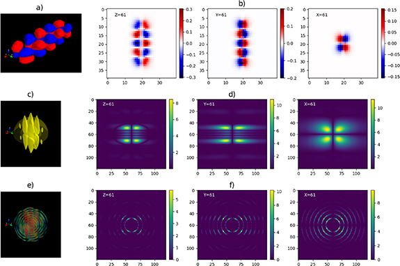
Figure 2. (a), (c), (e) Visualization of a 3D molecular orbital in the physical domain, Fourier domain and as measured on a set of spheres, respectively; (b), (d), (f) exemplary slices of (a), (b), (c) at three axes.
Download figure:
Standard image High-resolution imageWe take as the starting point of our algorithm a photon-energy-dependent set of momentum maps. The details on how these momentum maps are acquired differ from one experimental facility to the next; for example, the data structure as retrieved using a toroidal analyser [35] can be subtly different [36] to what would be measured using a time-of-flight momentum microscope [21–23, 27, 37]. For simplicity and generality, we will therefore assume that we extract from the measurement a two-dimensional intensity distribution  for the coordinates (
 ) with for
  . Furthermore, we will assume that the measured intensity distribution is already corrected for the polarization factor
  (c.f. equation (1)).
Each of these momentum maps is a measurement of the intensity on a hemisphere, which can be completed to a sphere by applying the symmetry expected from a real-valued object, i.e. the molecular orbital. The momentum maps are therefore spheres in the data domain  with radius
  depending on the photon energy
  used for photoemission; these data spheres are denoted
  . The value of r is determined by the experimental parameters and must be mapped to the voxel grid described above. We index the various measurement spheres with the symbol ρ so that the voxels corresponding to the measurement sphere with radius rρ
are indicated by
. The value of r is determined by the experimental parameters and must be mapped to the voxel grid described above. We index the various measurement spheres with the symbol ρ so that the voxels corresponding to the measurement sphere with radius rρ
are indicated by  . Since a sphere with radius r will run through voxels with an inherent thickness, the measurement sphere will inherit this thickness through the discretization. Complicating matters further is the fact that the measurement device is a planar array, i.e. that kz
is not directly measured. All of these effects of discretization and projection onto a planar grid can be accounted for approximately by an appropriate scaling of the measurements. Accounting for this explicitly in the discussion below adds notational clutter that obscures the main ideas, so we will suppress these specifics in our presentation. Instead, interested readers may refer to the related data repository [38], which includes the script that was used to cast ARPES measurements to
. Since a sphere with radius r will run through voxels with an inherent thickness, the measurement sphere will inherit this thickness through the discretization. Complicating matters further is the fact that the measurement device is a planar array, i.e. that kz
is not directly measured. All of these effects of discretization and projection onto a planar grid can be accounted for approximately by an appropriate scaling of the measurements. Accounting for this explicitly in the discussion below adds notational clutter that obscures the main ideas, so we will suppress these specifics in our presentation. Instead, interested readers may refer to the related data repository [38], which includes the script that was used to cast ARPES measurements to  .
.
A 3D-POT data set containing momentum maps at m photon energies then provides measurement data on m spheres with radius rρ
for  . The measurement spheres taken together are denoted by

is the corresponding collection of voxels. The equation (1) can be reformulated in the following form, as presented in, for example, [39, 40]:

where

The problem we are faced with is to find ψ that is consistent with the relationship (3), i.e. find ψ when we know only the amplitude of its Fourier transform on finitely many spheres in momentum space. This is a type of phase problem where the data is sparse and restricted to spheres in the Fourier domain. The new challenge is to retrieve not only the phase of the measured data but also the phase and Fourier magnitude on the missing voxels  . Only by accomplishing this can the complete molecular orbital ψ be calculated.
3.2. Model and method
3.2.1. Model
The phase retrieval problem has a rich history and many different approaches to its solution. The algorithm we use here is the most prevalent and successful for phase retrieval and is based on a non-convex feasibility model [40]. As explained above, the 3D-POT data records the momentum distribution of a specific molecular orbital on set of spheres. The first step in the feasibility model approach is conceptual: we view the data as specifying a set of orbitals ψ that could have produced the data; i.e. any ψ consistent with the data is acceptable. We will not belabor the transition in thinking about ψ and  as functions taking values on D (respectively
  ) to their discretized versions as vectors in
  and
and  . This allows us to write
  instead of
  ; likewise
  corresponds to
  . The set of points ψ satisfying (3) in this discretized form is thus defined by

where  is defined by (2). This of course leads to too many possibilities, so we narrow the options down by adding other constraints or prior knowledge about the orbitals.
The first constraint concerns the experimental resolution in real space. To ensure that the full measurement data can be included in the analysis, the domain  is chosen to be large enough to fully contain the data for the highest photon energy, which lies on the shell
  with the maximum radius
  . Consequently, the corners of
  lie outside the measured area in momentum space. As the momentum distribution in the corners is not constrained by the measurement, and an overestimation of the intensity can lead to high-frequency noise on the reconstructed orbital, we set the intensity outside of the shell
  to zero. This reflects simultaneously the experimental limitations as well as bandwidth limitations on the types of orbitals which can be successfully recovered. More will be said about this below when we impose symmetry constraints on the orbital, but imposing such a bandwidth constraint is equivalent to applying a low-pass filter in momentum space at the determined experimental resolution. Let
  be a ball in momentum space
  that contains all measured spheres Sj
(
that contains all measured spheres Sj
( ) in the Fourier domain. The set of orbitals satisfying the bandwidth constraint is given by

The following constraints concern the properties of the molecular orbital in the object domain D. Let s > 0. In the object domain D, we utilize a sparse-real constraint which is defined as follows:

where, Im is the imaginary part of the complex vector ψ, and
  denotes the counting function that counts all non-zero voxels. We employ the sparse-real constraint since the molecular orbital that we are recovering consists of a small number of positive and negative-valued lobes (e.g. figure 2(a)). Sparsity constraints were first employed in phase retrieval by Marchesini in [41], and have previously been applied successfully in orbital imaging [8]. The sparsity constraint imposed by the restriction on the value of the counting function allows us to impose a movable support constraint on the orbitals; this is very convenient since we do not know the molecular orbital initially, and the counting function allows the support to evolve during the reconstruction process. This constraint therefore also eliminates the need for a shrink-wrap procedure to fine-tune an a-priori unknown object support [5, 42].
It is not uncommon that the symmetry of a given molecular orbital is known in advance. Based on the properties of the orbital shown in figures 2(a) and (b), we introduce additional assumptions, namely symmetry and anti-symmetry constraints. The set of points that are symmetric about the x-axis, anti-symmetric about the y-axis, and anti-symmetric about the z-axis is denoted as SYM and is expressed as follows:

Imposing a symmetry constraint in the object domain D is made more challenging by the fact that the magnitude of the Fourier transform is invariant under spatial shifts in the object domain. Reconstructions that are consistent with the measured data, and even the sparse-real constraints can appear anywhere in the object domain D (see figure 3(e)). While we might see symmetries in the reconstruction with our eyes, to impose these as a constraint we need to align the object with an axis of symmetry (see figure 3(d)). We accomplish this by simply applying a conventional, fixed support constraint (as opposed to the sparsity support constraint above) centered at the origin that is symmetric in each of the x, y, and z directions separately. We emphasize that the size of this support is chosen small enough to ensure proper alignment of the object, but also large enough that it does not affect the shape of the ultimately reconstructed object. This is shown in figure 3(b). Given a symmetric binary mask  , the support constraint set is denoted SUPP and given by

We refer to the mask Ω as the support region. By using the support constraint, we can not only avoid spatial translation of the recovered object, but also speed up the recovery process by reducing the number of indices that need to be estimated.
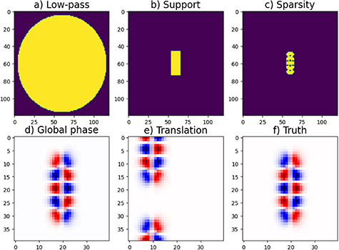
Figure 3. Visualization of (a) the ball  bounding the low pass region in the Fourier domain. The updated Fourier modulus on the dark background will be set to zero, see (6); (b) the support region which limits the updated value only inside the light box and is applied in real space; (c) the sparse real constraint sets amplitudes below a dynamic threshold to zero, allowing us to obtain a tighter support. (d) and (e) show typical ambiguities of the measurement constraint: (d) shows a change in sign and (e) is an example of a translation, which can make it difficult to apply symmetry constraints. (f) shows the true molecular orbital.
Download figure:
Standard image High-resolution imageHaving defined the qualitative constraint sets above, we can now formulate the feasibility model as finding a point that lies in all these sets:

This is an inconsistent problem because the qualitative constraints are idealized and the intersection above is empty. From a physical perspective, the most significant impediment is due to the fact that the true molecular orbital in Fourier space is actually non-zero outside the ball  . From a numerical perspective, different sparsity parameters s in (7) or support regions Ω in (9) may also cause inconsistency, as they introduce hard edges which are suppressed by the low-pass filter LF. Inconsistent feasibility has been studied in [43] where the interpretation of ‘solutions’ to (10) is explained in terms of difference vectors or gaps of smallest magnitude between successive sets [43, lemma 3.2]; this is depicted in the case of two sets in figure 4. Generally, it is found that the size of the gap correlates with the distance to the ‘true’ solution, such that the reconstruction with the smallest gap provides the best approximation.
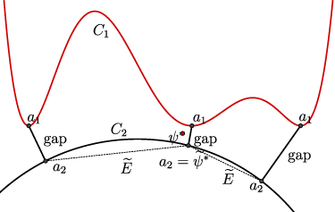
Figure 4. Example of a non-convex and inconsistent problem involving two sets, C1 and C2. The nearest points between the sets C1 and C2, denoted as a1 and a2 respectively, are shown. Depending on where the starting point  is picked, we obtain different solutions a1 and a2.
Download figure:
Standard image High-resolution image3.2.2. Method
Algorithms based on metric projections are the most successful methods for finding points where the gap between the sets is smallest [40]. The Cyclic Projection algorithm (CP) is one of the simplest, and more effective approaches. Since the focus of this work is not on the algorithms, we will limit ourselves to CP; if the reconstructions are successful for cyclic projections, they will also be successful for more sophisticated algorithms. The algorithm CP is given by:

Here  denotes the reconstructed orbital at the nth iteration and PC
denotes the metric projector onto a set C. The formulas for the individual projectors are given in the supplementary information.
denotes the reconstructed orbital at the nth iteration and PC
denotes the metric projector onto a set C. The formulas for the individual projectors are given in the supplementary information.
Luke et al [43, theorem 3.2] proved guarantees on local linear convergence of CP to fixed points, i.e. points  with
with  , for non-convex problems and global linear convergence for convex problem under regularity assumptions of the sets. In short, for our non-convex problem, as long as the starting point is close enough to a fixed point of the algorithm, then the iterates of the algorithm converge linearly to a fixed point.
3.2.3. What to monitor?
To decide when to stop the algorithms, we define:

where  for all
  . The iterations are terminated once the distance between successive iterates computed by (12) reaches a tolerance, for example
  . The theory [43, example 3.6] establishes that algorithm (11) converges locally linearly for this problem; how long one needs to wait until a region of local linear convergence is found, however, is undetermined. The simplest solution is therefore to wait until the expected local convergence behavior is observed. Figures 5(a) and (b) show that the range of possible iteration counts before local linear convergence is observed remains relatively stable under changes in other model parameters, like the number of spheres, or the sparsity parameter.
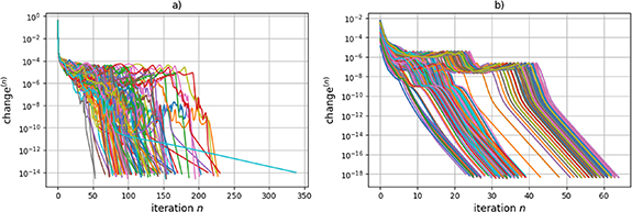
Figure 5. Algorithm performance of locally and globally random initialization. (a) Iterate differences of 100 globally random initializations (b) Iterate differences of 1000 locally random initializations.
Download figure:
Standard image High-resolution imageIterates of the cyclic projection algorithm (11), and in particular final iterate, always belong to the set SYM but not necessarily to the other sets. However, we can always look at the intermediate points from the sets SR, SUPP, LF or M simply by storing these intermediate projections. Specifically, if  is the retrieved orbital obtained after completing the iterative process, the ‘shadow’ of this point on the set
  is calculated by
  ; the corresponding shadow on the set
  is computed by
  , and so forth. Depending on the application, one might prefer one ‘shadow’ over other possible shadows for the reconstructed orbital. In this paper, we opt for reconstructions on the
  set because they do not retain artifacts due to, e.g. measurement noise. Some practitioners take averages of reconstructions on all sets; we do not recommend this because the mathematical interpretation could be lost, but in the end, this decision is application dependent.
For the simulated 3D-POT analysis we denote the truth, which is the Kohn–Sham molecular orbital that is used for the data simulation, by  . As mentioned earlier, problem (10) is inconsistent, and thus, the point that solves (10) in some sense is not
  , but rather a point close to it; this ‘best numerical solution’ is denoted
  . There are different ways to define this point. We explain our approach to this issue in more detail in the next section. Regardless of how one defines
  , we have the following errors:

and

where  denotes the preferred shadow of the reconstructed orbital at the nth iteration. The best numerical solution
  is constructed so that it belongs to the same set. The error is the minimum of either the sum or the difference of the reconstruction and the reference ‘truth’ to account for the unavoidable global phase ambiguity, e.g. the change in sign, shown in figure 3(d). The formula (13a
) is the error between the reconstruction and actual orbital. This metric helps us to estimate reliability of the model. On the other hand, formula (13b
) tells us how far the algorithm is from the best numerical truth to the model problem. Thus, the model error (13b
) could be small, while the physical error (13a
) is large; in this case, it may be necessary to consider adding additional constraints or modifying the model. It is easy to see that
is constructed so that it belongs to the same set. The error is the minimum of either the sum or the difference of the reconstruction and the reference ‘truth’ to account for the unavoidable global phase ambiguity, e.g. the change in sign, shown in figure 3(d). The formula (13a
) is the error between the reconstruction and actual orbital. This metric helps us to estimate reliability of the model. On the other hand, formula (13b
) tells us how far the algorithm is from the best numerical truth to the model problem. Thus, the model error (13b
) could be small, while the physical error (13a
) is large; in this case, it may be necessary to consider adding additional constraints or modifying the model. It is easy to see that  for all
  . Moreover, when the model fits perfectly with the truth, i.e,
  , we get
  .
.
The accuracy of the reconstructed orbital is also influenced by the initial starting point, given the non-convex nature of the problem. While in simulation it is trivial to compare the reconstructed orbital and the truth, this is not possible in experiment. Thus, there is a challenge in selecting the best reconstruction among the multiple possibilities. To address this challenge, we monitor the sum of the gaps between the sets at any given iterate:

where
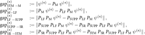
When the algorithm converges, the gap remains constant but nonzero. For a sufficient number of trials, the reconstruction with the smallest gap corresponds to the point where the different constraints are nearest to each other. If the model of the molecular orbital is reliable, then it is likely that this point provides the best approximation of the true solution (see figure 4). However, a smaller gap does not necessarily have to imply a smaller error. In our numerical experiments, we will investigate to what extent the gap can be used as a measure for the reconstruction accuracy.
4. Numerical results
The implementation of algorithms described in this section can be downloaded from the link [38].
Starting with the highest occupied molecular orbital of an isolated pentacene molecule as calculated by DFT (figure 2(a)), we generated 3D-POT data for up to 56 photoelectron kinetic energies in the range up to 110 eV such that the spheres are equidistantly spaced in momentum. This high photoelectron kinetic energy enables a high spatial resolution in the reconstructed image, but we emphasize that such a high energy is not necessary to achieve 3D orbital images. This is also demonstrated in the supplementary material, where we achieve similar reconstruction results to those presented below using a photoelectron kinetic energy up to 30 eV. The individual momentum maps span a momentum range of  Å−2 with
  pixels (although our simulated measurement data only covers the central part of the image up to a 5.5 Å−1 radius). From these momentum maps, we calculate the measured intensities
  in the data domain
  , which has dimensions
  . Each voxel in
  therefore has a volume
  Å−3. Since the orbital is real-valued, we set the intensities
  . To define the symmetric support region Ω in the object domain D, we chose a shape of
  voxels (
 Å3) located at the center of the image. The radius of the low-pass filter
  is set to
  (= 5.5 Å−1), as shown in figure 3(a) for the 2D case; as claimed, the bandwidth contains all the spheres for which we simulated measurements to perform the reconstructions. We start with ideal data, generated using a fixed total number of 1012 detected photoelectrons with constant, well-calibrated vector potential A (i.e. the probe light intensity).
4.1. Convergence
In figure 5, we investigate the convergence behavior under various scenarios. Frame a) shows 100 globally random instances (i.e. the starting points are chosen randomly over the entire domain space) of the algorithm behavior with a fixed sparsity value s = 3360 and fixed data including all m = 56 measured spheres. All instances exhibit local linear convergence, as expected. The variation of the slopes of the graphs in this frame indicates considerable heterogeneity of local minima. In our experiments, we observed no correlation between the rate of convergence of the algorithm and the quality of the local minima. It is interesting to observe in frame b) the convergence plots of 1000 locally random instances using data m = 56 and s = 3360, i.e. instances whose starting points are randomly chosen in a small neighborhood of a fixed point. Here, we specifically select the neighborhood around the starting point of the best numerical reconstruction,  . Most of the graphs have the same slope in the final iterations, indicating a constant of linear convergence concentrated around the value
  , and its variance is only
  . This indicates that the geometry of the problem around this local minimum is not wildly varying; a mathematical statement about why this should be the case is beyond the scope of this work. As argued in [44], under the assumption of Q-linear convergence, the rate of convergence r of each instance can be estimated empirically from the observed local numerical behavior. Here, we observe that the mean of r is approximately 0.28 with a small variance of about
  . Moreover, the average error
  over 1000 reconstructions is
  with a variance of about
  , suggesting that the fixed point with the smallest gap is an isolated point, which further bolsters the hypothesis that numerical convergence is Q-linear.
In order to benchmark the reconstruction depending on various parameters such as the sparsity parameter, the number of photon energies and the intensity calibration, we now define the best numerical solution  , which may be referred to as the ideal reconstructed orbital for the inconsistent problem (10). This is constructed with the fixed point of algorithm (11) obtained using data from 56 spheres of ideal data with the setting s = 3360 in figure 5(a); note that we constructed
  so that it belongs to the set SYM, and from 100 globally random initializations it was chosen as the solution that achieved the smallest gap. The errors that we report are the distances between points computed by the algorithm in the set SYM. The distance between the truth and the best numerical solution, i.e.
  , is 7.4%.
In the following section (4.2), we present exemplary numerical results that demonstrate the successful reconstruction of the orbital using as little as m = 4 photon energies. In section 4.3, we then conduct a more comprehensive investigation of the effects of the sparsity parameter s, the number of spheres m, the starting points, and calibration errors (defined below), exploring their impact on the reconstructions.
4.2. Example: 4 photon energies
Figure 6 shows the results of typical reconstructions using m = 4 spheres (radii: 1.9, 3.2, 3.9 and 4.6 Å−1, photoelectron kinetic energies 13.1, 39.6, 58.2, and 80.3 eV, respectively) of ideal data and sparsity s = 3360 at two different starting points, in comparison to the ideal reconstructed orbital. Here, one point, denoted ψ1, achieves an error of  , while another point, denoted ψ2, achieves
  . These reconstructed orbitals are selected from a pool of 100 experiments with varying starting points. The reconstruction ψ2 is the result with the smallest gap among the 100 random initializations; ψ1 is just a randomly selected trial.
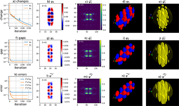
Figure 6. Comparison of retrieval results ψ1 (blue lines, panels (b)–(e)), ψ2 (orange lines, panels (g)–(j) at two different starting points using ideal data on m = 4 spheres with the best numerical solution  (panels (l)–(o)). The sparsity is set to s = 3360. The reconstructions have been normalized by dividing them by their norms for the purpose of visualization.
Download figure:
Standard image High-resolution imageFrame (a) of figure 6 shows that the algorithm is converging at a locally linear rate on termination for both instances, as expected. In frames (f) and (k), it is clear that the quality of the reconstructed orbital is affected by the choice of starting points, as measured by the gap and the error, respectively. The fact that the gaps and errors appear unchanged from iteration 500 onward does not necessarily indicate that the solutions have stopped changing, as indicated in frame (a). Our objective is to find a point whose corresponding difference vectors are as small as possible; by this reasoning, the better solution should be ψ2 (orange) as it corresponds to the reconstruction with the smallest gap. Indeed, visual inspection of the constant height (z) maps in frames (b), (g), (l), the constant kz maps in frames (c), (h), (m) and the isosurfaces in frames (d), (i), (n), (e), (j), (o) confirms that ψ2 is a better approximation of the molecular orbital. Further experimental results regarding the relationship between the gap and error can be found in the next subsection.
4.3. Reconstruction accuracy in experiment
In section 4.2 we have seen that, although good orbital reconstructions can be achieved using the CP algorithm for 3D-POT, not all random starting points yield the same reconstruction accuracy. In order to investigate how the best results can be achieved, it is first useful to characterize the impact of the sparsity parameter s on the reconstruction result since the sparsity parameter is one of the few control parameters that the user can easily adjust. In this context, also the size (whether larger or smaller) of the support or low-pass filter LF may impact the quality of the reconstruction. In particular, without a low-pass constraint at all, the algorithm tends towards orbitals with un-physically strong high-frequency components. However, a detailed discussion of the effects of the low-pass and support constraints is beyond the scope of the present paper.
4.3.1. The sparsity parameter s
In figure 7(a), we present the dependence of errors E and  on the sparsity parameter s for a dataset consisting of m = 56 input spheres of ideal data. Each s value underwent testing through a total of 100 globally random trials (i.e. we use the same reconstructions as in figure 5(a)). We then calculated the averages of E and
  across these starting points. We also identify the minimum values of E and
  among the 100 trials for each value of s. Here, the minimum achieved error provides an indication of the reconstruction quality that can be achieved, while the mean and spread show that a significant number of trials is necessary to achieve the best result.
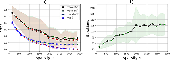
Figure 7. Dependence of (a) errors E and  on the sparsity parameter s, and (b) the average number of iterations needed to achieve convergence using ideal data, setting m = 56. The data points indicate the mean error and minimum achieved error (out of 100 trials), while the shaded regions indicate the standard deviation: in frame (a) the green shaded region is the standard deviation of E, the pink-shaded region is the standard deviation of
  and the brown shading indicates the overlap. How these results were obtained is described in section 4.3.
Download figure:
Standard image High-resolution imageFigure 7(a) shows a trend that the number of required iterations increases as the number of nonzero voxels s increases, while the error decreases as s increases. This holds for both the mean and the minimum errors of E and  . The data shows that a wide spread of reconstruction errors is to be expected for all s. Therefore, it is necessary to perform reconstructions with multiple globally random instantiations and select the best one. In order to achieve the most accurate reconstructions in the following part of our investigation, we set the sparsity parameter to s = 3360, where the size of the support constraint matches s.
Figure 7(b) displays the average number of iterations until convergence over 100 trials, corresponding to the data presented in figure 7(a) for each sparsity level s. A smaller value of s results in a faster reconstruction process and a smaller spread. The average number of iterations remains the same when s is large, but there is a larger relative variation.
4.3.2. Number of spheres
As the number of photon energies and thereby measured spheres increases, the algorithm is provided with more information and needs to fill fewer voxels. In figure 8(a), we run a total of 500 reconstructions using ideal data with a fixed sparsity parameter s = 3360 for five settings of m:  . The m = 4 data includes the same spheres as described in section 4.2, the m = 7 data covers radii of 1.2 to 5.2 Å−1 (5.2, 13.1, 24.6, 39.6, 58.2, 80.3, and 106.1 eV kinetic energy), and the
  data sets cover radii of 0.5 to 5.4 Å−1. Again, each value of m was tested with 100 globally random instances.
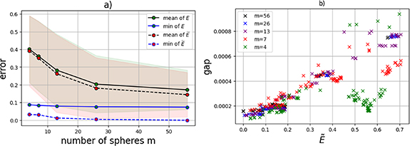
Figure 8. Correlation between (a) number of spheres m and errors E,  and (b) gap and error
  using a varying number (m) of spheres, setting s = 3360, 100 globally random initialization for each m, for well-calibrated data.
Download figure:
Standard image High-resolution imageSimilarly to figure 7(a), we measure the mean values of E and  , along with their spreads and respective minimum values, and find that the mean errors decrease as the number of measurements increases. Moreover, the decrease in spreads indicates that the errors exhibit less variation when more data is used. Also as expected, the error measured against the best numerical solution,
  , goes to zero as the number of shells increases to 56.
Rather surprisingly, whereas the mean E and  increase significantly as the number of spheres is reduced, the minimum error increases much less. For all numbers of spheres, the minima of E and
  stay below 0.1. This observation leads to the conclusion that a dense input is not necessary; using
  or even 4 shells can still yield a close approximation of the orbital as long as a sufficient number of trials is performed. Finally, we note that the simulated data for
  also includes photoelectron kinetic energies below 5 eV which are often inaccessible in experiment, e.g. due to strong final-state effects or the presence of a strong inner potential [45]. To verify that the inclusion of these shells in the reconstruction does not affect our conclusions, we have also performed reconstructions where we exclude shells for which the photoelectron kinetic energy is less than 14 eV. From this analysis, we find that the exclusion of these shells leads to an increase of the best feasible error of less than 10−3 from
  to
to  . We thus conclude that the lower kinetic energy shells do not affect the reconstruction strongly.
In all of these numerical experiments, we chose the photon energies such that the radii of the corresponding spheres are evenly spaced in momentum (for example, see in figures 2(e) and (f)) for the case of 7 spheres). It is possible that the energy spacing can be adapted to the specific molecular orbital of interest to provide better reconstruction results, however this falls outside of the scope of the present study.
In section 4.2, we have observed an example where examining the gap can offer insights for selecting a reconstruction when both the ground truth and the ideal reconstruction are unknown. Using the full dataset of 500 numerical reconstructions with different m, we can investigate more quantitatively to what extent the gap can be used as an indication for the error E (or  ). In figure 8(b), we depict the dependence of the gap and
  for each random instance and input data m. First, we note a clear trend in the data, where a larger error
  generally corresponds to a larger gap. Surprisingly, this trend is highly similar between datasets with different m. We emphasize that this match between different m is not expected to be general, but in this case it further supports that there is a direct correlation between the error
  and the gap. However, we also observe that the correlation between the gap and
  weakens as the amount of data decreases; this is particularly true for m = 4. This is because the problem becomes more ill-defined and, therefore, more non-convex. Still, even for m = 4 the smallest gaps do result in the smallest
  as claimed.
4.3.3. Intensity calibration
In experiment, measuring 3D-POT data requires to tune the photon energy to a range of values and to measure the photoemission rate normalized to the amplitude of the incident light field. Consequently, a precise calibration of the—often fluctuating—extreme ultraviolet (EUV) light intensity is necessary. If fluctuations in the EUV power are not properly accounted for, calibration errors may arise which scale the measured intensity on individually measured spheres with respect to the true momentum distribution of the orbital. Furthermore, it is well known that the plane-wave model of photoemission (equation (1)) does not always provide a good prediction of the photon energy dependence of the photoelectron spectrum [30, 46], which can lead to similar errors in the measured momentum distribution. To assess how sensitive the algorithm is to such model miss-specification, we now add EUV intensity calibration errors to the data.
Let  , the number of spheres. Let
  be a uniformly distributed random sample of lengths m in the interval (0, 1), and let
  . For
. For  , the ideal data is distorted by following formula:

where  . Then
  and we get

We refer to b′ as calibrated data. Let α be chosen from the set  ; α has the interpretation of a measurement accuracy or miss-specification level, so these numbers correspond to maximal noise or miss-specifications of 10%, 20%, 30%, 60%, and 90% for each sphere, respectively. To clarify, for α = 0.1, the average photon flux at each photon energy is measured with an error margin of
  .
.
For each m, we generated 10 samples  yielding 50 datasets for each value of m across the respective levels of α. We add 1 ideal dataset (with α = 0) for each m. This results in a total of 255 datasets.
We study the behavior of the algorithm, for fixed algorithm parameters, under the realizations of calibration error as described above. The results displayed in figure 9 show the recovery performance, indicated by the error with the best numerical solution  defined by (13b
), over
defined by (13b
), over  reconstructions with a fixed s = 3360 (i.e. 100 globally random initializations per simulated dataset). The average number of iterations required for convergence for
  was about
  iterations, respectively.
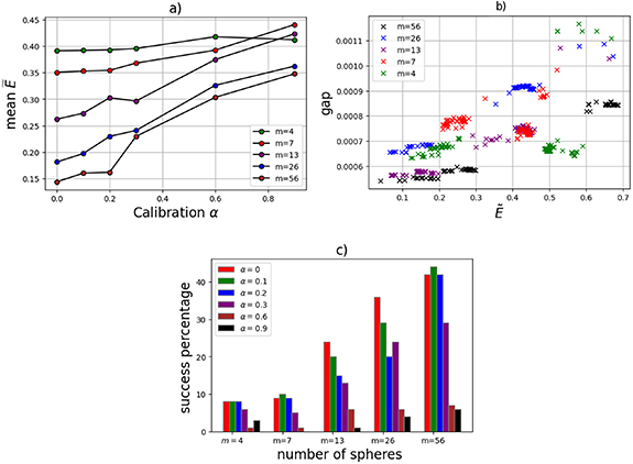
Figure 9. (a) The average value of  as a function of calibration error α; (b) the correlation of gap and
  with α = 0.6; (c) The dependence of success percentage (
 ) on m and α.
Download figure:
Standard image High-resolution imageFigure 9(a) provides an overview of the average of  depending on m and α. As expected, we observe a decrease in mean error both as the data becomes more accurate (i.e. as α decreases) and as the data becomes richer (i.e. as m increases). Note that for m = 4, the dependence of the mean
  on α is relatively weak. This surprising result has a relatively simple explanation: at m = 4, the model already allows for so many false local minima, that the added complexity due to model miss-specification does not worsen the results significantly.
However, these results also show that the mean error is not enough to characterize the algorithm performance. In the following, we define that a given reconstruction is successful if it has an error  (i.e. when the error is below 10%). At this error level, the reconstructed isosurfaces all match well to the true molecular orbital. Strikingly, in figure 9(c), we find very similar success rates for
  as for ideal data with α = 0. The success rates are slightly reduced, but a series of 100 globally random initializations is still likely to retrieve several successful reconstructions, which can then be selected by means of the minimum gap. For larger values of α, the data becomes significantly more inaccurate, resulting in a marked decrease in the percentage of success. Nevertheless, even in these cases a few successful reconstructions are found.
From a numerical perspective, this shows that systematic model errors like calibration error do not eliminate physically meaningful reconstructions (interpreted as global minima), but such errors do introduce more local minima that are less meaningful. Furthermore, the miss-specification of the model affects the correlation between the gap and the error, as shown in figure 9(b). For larger miss-specification (here observed for α = 0.6 with  ), the gap can no longer be used to select the best reconstructions, however we emphasize that we have only encountered this problem for very large miss-specification level which are not realistic in experiment. We therefore conclude that the algorithm is robust in the presence of the calibration error. Optimal results of course require the best possible intensity calibration, but significant errors up to 30% in the amplitude of the momentum distribution are not detrimental.
From the perspective of condensed matter physics, the observation that these light-intensity calibration errors do not strongly affect the chance of reconstruction success is very surprising. Indeed, if the amplitude of the momentum distribution is scaled in a certain region, then a Fourier transform will show that also the real space molecular orbital has been modified. In this case, however, we find that the cyclic projections algorithm can suppress the effect of such scaling in momentum space. Due to the hemispherical shape in momentum space of each ARPES measurement, any intensity miss-calibration will scale the amplitudes in a spherically symmetric manner. In real space, this corresponds to convolution with a spherically symmetric point spread function, blurring and modifying the molecular orbital in all 3 directions. Both the support and sparsity constraint can suppress this blurring, and thereby effectively correct for the intensity calibration error. Hence, it is possible that the sensitivity to calibration errors is increased if the support region (or sparsity constraint) is less accurately known.
4.3.4. Number of electrons
Next to the calibration errors that were discussed above, an important source of model inconsistency is intensity noise in the measured momentum maps. Precisely how the momentum maps are acquired differs per experimental setup; however a common factor to all ARPES experiments is electron counting statistics. Here, we compare the effect of reducing signal-to-noise ratio of the data on the quality and reliability of the reconstructed orbitals by simulating datasets with varying total photoelectron counts. Other possible sources of experimental noise, such as background noise or the aforementioned calibration error, are neglected. Each of the datasets in the previous numerical experiments were generated with 1012 photoelectrons, which is large enough that the data can be assumed to be noise-free. For this experiment, we now generate a dataset including m = 7 photon energies using instead a total of 105 detected photoelectrons (see figure 10 for an exemplary simulated ARPES map).
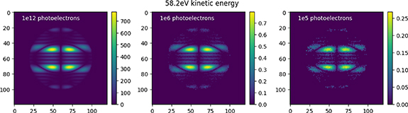
Figure 10. Exemplary simulated ARPES momentum maps from the m = 7 data for different number of photoelectron counts.
Download figure:
Standard image High-resolution imageAt this signal strength, the measurement data is significantly affected by Poissonian noise, and a significant fraction of the voxels that would otherwise indicate a low intensity now are zero: where in the noise-free case 6.4% of the voxels in the data domain are non-zero, this reduces to 1.6% at 105 counts. Nevertheless, the orbital reconstruction is not significantly impacted: As before, we fixed s = 3360, conducted reconstructions with 100 globally random starting points, and found that in this case a success rate 7% (i.e. with  ). With 106 incident electrons, where 3.1% of the voxels is nonzero, the percentage success increases slightly to 8%. We emphasize that these total photoelectron counts are very easily achievable with all of the currently used photoemission orbital tomography detectors. Our results therefore indicate that efforts towards achieving higher data quality should be aimed at reducing other experimental noise factors, such as the determination and subtraction of background signals.
4.3.5. Symmetry
Finally, we discuss the effect of the symmetry constraint on the reconstruction algorithm. We find that symmetry provides a strong constraint that greatly affects the efficiency of the algorithm and the number of local minima. Reconstruction algorithms without symmetry constraint, or with a reduced symmetry constraint, typically require significantly more iterations to fully converge. Nevertheless, such reconstructions do converge, and also recover the same minima found with the symmetry constraint. For the m = 13 data presented above, we find that these reconstructions find the correct symmetry of the molecular orbital.
In order to verify that the algorithm can also recover intrinsically asymmetric molecular orbitals, we will now consider the highest molecular orbital of a strongly bent PTCDA molecule, which was previously found to occur on the MgO(001)/Ag(001) surface [13]. Figures 11(a) and (b) shows the molecular orbital as calculated by DFT; it can be seen that the orbital is anti-symmetric in both the x and y directions. To perform orbital imaging in this challenging case, we simulated 3D-POT data for 13 photon energies, corresponding to kinetic energies ranging from 2 to 76 eV. Typical momentum maps at fixed photon energy are shown in figures 11(d) and (e). For the reconstruction, it is necessary to adapt the support, sparsity and symmetry constraints. We set the support constraint to  voxels (
 Å3), set the sparsity to s = 1344 and adapt the symmetry constraint for the symmetry indicated above.
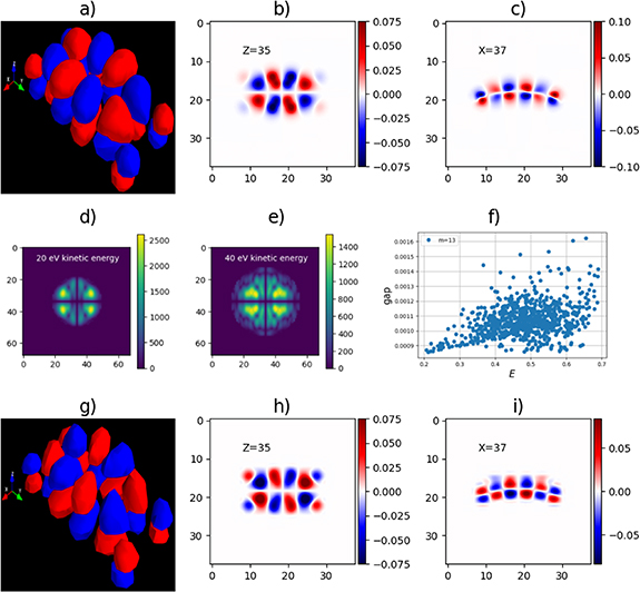
Figure 11. 3D orbital imaging of a non-symmetric molecular orbital. (a) Highest occupied molecular orbital of a bent gas-phase PTCDA molecule, from [13]. (b), (c) Slices at constant height (z) and at fixed x, showing the curvature of the molecule. (d), (e) Exemplary momentum maps of the simulated 3D-POT data. The full simulated dataset contains 13 hemispheres. (f) Relation between gap and error for 800 globally random initializations of the reconstruction algorithm. (g) Isosurface of the best reconstruction with E = 0.21. (h), (i) Exemplary slices at constant z and x of the best reconstruction confirm that the reconstruction algorithm recovers the bent nature of the molecule. These slices were interpolated for visualization only.
Download figure:
Standard image High-resolution imageFigures 11(f)–(i) show the results of 800 reconstructions with globally random initialization. Out of these reconstructions, we find that the best reconstruction achieves an error with respect to the true orbital of E = 0.21. (Note that we did not determine the best numerical solution in this case.) From figures 11(g)–(i), it is clear that the algorithm faithfully reproduces the curvature of the molecule. These results clearly show that also highly non-symmetric molecular orbitals can be reconstructed from 3D-POT. We expect that the reconstruction error can be further reduced by relaxing or adapting the support and sparsity constraints if needed.
We emphasize that a symmetry constraint is highly beneficial for eliminating bad local minima, and for getting in the neighborhood of physically meaningful reconstructions. Judicious application of symmetry can be very effective even when it does not (precisely) hold: in these cases, an initial reconstruction with symmetry can be used to provide an initial guess for the reconstruction without symmetry.
5. Conclusions
In this paper, we have addressed the challenge of reconstructing full 3D molecular orbitals from sparsely sampled 3D photoemission orbital tomography data. We propose a feasibility model and utilize the cyclic projections method to reconstruct the orbital. The model incorporates prior constraints such as low-pass filtering, support, voxel sparsity, and symmetry properties. Although this leads to an inconsistent feasibility model, we show that the global minimum closely approximates the true solution, which can be found with reasonably high probability by initializing the algorithm at several randomly chosen points and selecting the reconstruction with the lowest gap-value.
Remarkably, we find that the iterative orbital reconstruction method works for both symmetric and non-symmetric molecular orbitals, can deal with very sparse data, and is robust in the presence of crucial experimental noise factors such as the light intensity calibration and the total signal strength. In particular, a 3D-POT dataset covering only four photon energies in the EUV range already allows for accurate orbital reconstruction with over 8% of the reconstructions achieving an error  within 90% of the best possible value. This indicates that the orbitals to be reconstructed are sparse in some representation (e.g. spherical harmonics). Future research will investigate how to exploit such sparse representations.
Our results are especially promising in the context of laboratory-based, table-top photoemission orbital tomography, where high-harmonic generation EUV light sources provide access to only a limited number of photon energies. The reduced measurement requirements also provide other opportunities, including potentially the extension to time-resolved 3D-POT [21–24]. A limitation of the method remains the relatively large variation in the results, as indicated by the standard deviation of errors in figure 7. This reflects a rather large variety of fixed points of the algorithm. Future work will investigate the performance of the this algorithm on experimental data, as well as exploring alternative numerical methods for solving the feasibility problem whose fixed point sets are verifiably smaller.
Acknowledgments
We thank Christian Kern and Peter Puschnig of the University of Graz for valuable discussions and for providing the DFT calculations of the bent PTCDA molecule. All authors were supported by the Deutsche Forschungsgemeinschaft (DFG, German Research Foundation)—Project-ID 432680300—SFB 1456 Collaborative Research Center 1456 program—Mathematics of Experiment, Project B01.
Data availability statement
The data that support the findings of this study are openly available at the following URL/DOI: https://doi.org/10.25625/LAT69R.