Abstract
We theoretically investigate first and second sound modes of a unitary Fermi gas trapped in a highly oblate harmonic trap at finite temperatures. Following the idea by Stringari and co-workers (2010 Phys. Rev. Lett. 105 150402), we argue that these modes can be described by the simplified two-dimensional two-fluid hydrodynamic equations. Two possible schemes—sound wave propagation and breathing mode excitation—are considered. We calculate the sound wave velocities and discretized sound mode frequencies, as a function of temperature. We find that in both schemes, the coupling between first and second sound modes is large enough to induce significant density fluctuations, suggesting that second sound can be directly observed by measuring in situ density profiles. The frequency of the second sound breathing mode is found to be highly sensitive to the superfluid density.
Content from this work may be used under the terms of the Creative Commons Attribution 3.0 licence. Any further distribution of this work must maintain attribution to the author(s) and the title of the work, journal citation and DOI.
1. Introduction
Low-energy excitations of a strongly interacting superfluid quantum system—in which inter-particle collisions are sufficiently strong to ensure local thermodynamic equilibrium—can be described by the Landau two-fluid hydrodynamic theory [1–4]. There are two well-known kinds of excitations, referred to as first and second hydrodynamic modes, which describe the coupled oscillations of the superfluid and normal fluid components at finite temperatures. First sound is an ordinary phenomenon in liquid, describing the propagation of a pressure or density wave that is associated with normal acoustic sound. The motions of the superfluid and of normal fluid components are locked in phase. In contrast, second sound is a phenomenon characteristic of superfluids. It describes the ability to propagate undamped entropy oscillations, which are essentially opposite phase oscillations of the two components. In the quantum liquid of superfluid helium, the velocities of first and second sound were first measured in 1938 by Findlay et al [5] and in 1946 by Peshkov [6], respectively.
Ultracold atomic Fermi gases near a Feshbach resonance represent a new type of strongly interacting quantum system with unprecedented control over interatomic interactions, dimensionality and purity [7]. These are anticipated to provide an ideal table-top system to deepen our understanding of fermionic superfluidity and Landau two-fluid hydrodynamics. For a Fermi gas at unitarity, first sound modes have been investigated in great detail, both experimentally and theoretically [8–17], particularly near zero temperature. In contrast, second sound mode is more difficult to address [18–27] and has only recently been observed in experiments [28]. Key to understanding second sound, is knowledge of the superfluid density [20, 29, 30], a quantity which is still a subject of intense investigation. Theoretically, first and second sound modes of the Landau two-fluid hydrodynamic equations were solved by Taylor et al for an isotropically trapped unitary Fermi gas [21], using an assumed superfluid density and by developing a variational approach. For general anisotropic harmonic traps, the Landau hydrodynamic equations are more difficult to solve. However, for a highly elongated configuration, it was shown by Bertaina, Pitaevskii and Stringari [24] that, a simplified one-dimensional (1D) two-fluid hydrodynamic description may be derived, generalizing the dimensional reduction at zero temperature [15]. Following this pioneering idea, the propagation of a second sound wave was strikingly observed in a highly elongated unitary Fermi gas by the the Innsbruck team [28]. Using the measured second sound velocity data, the simplified 1D hydrodynamic equations were solved and used to extract the superfluid density [28]. These results show that studies of second sound provide a promising route towards an accurate determination of the superfluid density.
Here, we would consider a unitary Fermi gas in highly oblate harmonic traps, which can be readily realised in current experiments. Indeed, such configurations have already been investigated in laboratory experiments [31–36]. The analysis presented here could therefore be directly tested in future experiments. Our main results are briefly summarized as follows. Following the ideas of Stringari and co-workers [24, 26], we derive the simplified two-dimensional (2D) Landau two-fluid hydrodynamic equations. Using a variational approach within the local density approximation [18, 20, 21], we fully solve the coupled 2D hydrodynamic equations in the presence of a weak radial harmonic confinement. The discretized mode frequencies of first and second sound are calculated. We find that the density fluctuation due to the second sound mode is significant, revealing that second sound is directly observable from in situ density profiles, after an appropriate modulation of the weak radial trapping potential. The mode frequency of second sound is found to depend very critically on the form of the superfluid density. Our quasi-2D analysis is similar to the quasi-1D study of Stringari and co-workers [26], however, there are a number of significant differences. Specifically we fully solve the coupled hydrodynamic equations without assuming that first and second sound are decoupled. This enables us to calculate the density fluctuations associated with the discretized second sound modes. From an experimental point of view, the possibility of measuring discrete breathing mode frequencies may allow a more accurate determination of superfluid density.
The remainder of the paper is organized as follows. In the next section, we outline the reduced 2D universal thermodynamics, satisfied by the unitary Fermi gas in highly oblate harmonic traps based on the measured three-dimensional (3D) equation of state [37]. In section 3, we derive the simplified 2D Landau two-fluid hydrodynamic equations and discuss very briefly their applicability. In section 4, we consider the propagation of first and second sound, which may be excited by creating a short perturbation of the density. The nature of first and second sound excitations in the quasi-2D unitary Fermi gas is described. In section 5, we fully solve the simplified 2D hydrodynamic equations and calculate the discretized breathing mode frequencies of first and second sound. The density fluctuation associated with low-lying second sound modes is discussed and the dependence of the second sound mode frequency on the form of superfluid density is examined. Finally, in section 5 we draw our conclusions. The appendix presents further details of our numerical calculations.
2. 2D reduced thermodynamics
Let us consider a unitary Fermi gas trapped in a highly anisotropic pancake-like harmonic potential

with atomic mass m and the radial and axial trapping frequencies  , ωz
. The aspect ratio of the trap, defined by
, ωz
. The aspect ratio of the trap, defined by  , can be specifically tuned in experiments. The number of atoms in the typical sound mode experiments [9, 10, 13, 16, 28] is about N ∼105. For such a large number of atoms, it is standard to use the local density approximation [7], which amounts to treating the atoms in the position
  locally as a uniform matter, with a local chemical potential given by,

Here μ0 is the chemical potential at the trap center. The validity of the local density approximation can be conveniently estimated by comparing the number of atoms N∼105 with a threshold  , below which there is a dimensional crossover from three- to two-dimensions [33, 34]. At Swinburne, we have previously demonstrated pancake traps with
  . Thus, the ratio
  , indicating that the system could be deeply in the 3D limit where the local density approximation is well justified.
2.1. Universal thermodynamics
A remarkable feature of a uniform unitary Fermi gas is that all its thermodynamic functions can be expressed as universal functions a single dimensionless parameter  [38, 39]. This is simply due to the fact that at unitarity, the s-wave scattering length—the only length scale used to characterize the short-range interatomic interaction—diverges. Thus, the remaining length scales are the thermal wavelength,

and the mean distance between atoms  , where n is the number density. Accordingly, the energy scales are given by the temperature,
  , and by the Fermi energy,

or, alternatively, by the chemical potential μ. Following the scaling analysis, all the thermodynamic functions can therefore be expressed in terms of universal functions that only depends on the dimensionless parameter  For the pressure and number density, these universal functions are given, respectively, by


Using the thermodynamic relation  , we find
  . It is easy to see that knowing
  and
and  , we can calculate directly all the thermodynamic functions of the uniform unitary Fermi gas [26].
It is highly non-trivial to theoretically determine the universal function  or
or  , since there are no small parameters to control the theory of a strongly interacting Fermi gas [40–44], except at high temperatures, where the virial expansion approach is applicable [45, 46]. Fortunately, accurate experimental data for the equation of state are now available from the landmark experiments performed by the Massachusetts Institute of Technology (MIT) team [37]. In figure 1, we present their data for the universal scaling function,
where the subscript ‘0’ indicates the result of an ideal, non-interacting Fermi gas and

For later convenience of numerical calculations, we have fitted the experimental data to an analytic expression, as detailed in appendix  is well-understood [23, 25, 45, 46]. As evident in figure 1, the relative error in the fitting is less than
  , significantly smaller than the standard error for the experimental data (i.e., 2%).
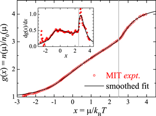
Figure 1. The universal scaling function of a strongly interacting unitary Fermi gas,  , where
  is the number density of an ideal spin-1/2 Fermi gas. The experimental data from the MIT team (red circles) [37] are compared with a smoothed fit (the black line), as described in the text. The inset shows the comparison for the derivative of the universal scaling function. The vertical grey lines indicate the critical threshold for superfluidity,
  [37].
[37].
Download figure:
Standard image High-resolution image2.2. Local density approximation
Within the local density approximation, we can write the local pressure and number density using the universal functions,


where the local chemical potential is given by equation (2). For a trapped Fermi gas in three dimensions, the Fermi temperature TF is defined as [7]

Using the number equation  , we relate
  to the reduced temperature
  by,
by,
The onset of superfluidity in a trapped unitary Fermi gas occurs at  . Numerically, we find that
  , in agreement with the previous results [26, 37].
2.3. 2D reduced thermodynamic functions
In highly oblate harmonic traps, although the cloud is still 3D, its low-energy dynamics are greatly affected by the tight axial confinement. This situation is very similar to a highly elongated unitary Fermi gas considered earlier by Bertaina, Pitaevskii and Stringari [24], who showed that with tight radial confinement, the standard Landau two-fluid hydrodynamic equations could reduce to a simplified 1D form. For the same reason, which will be explained in greater detail in the next section, first and second sound under the tight axial confinement can be described by a simplified 2D two-fluid hydrodynamic description. In brief, due to the nonzero viscosity and thermal conductivity, local fluctuations in temperature ( ) and chemical potential (
 ) become independent of the axial coordinate, for any low-energy excitations at the frequency
  . Therefore, the axial degree of freedom in all the thermodynamic variables that enter the Landau two-fluid hydrodynamic equations becomes irrelevant and can be integrated out. We can then derive 2D reduced thermodynamics and immediately have the reduced Gibbs–Duhem relation,

where the variables P2, s2 and n2 are the axial integrals of their 3D counterparts, namely the local pressure, entropy density and number density. The variable P2 is given by,
where
and we have introduced the universal scaling function,

All the 2D thermodynamic variables can be derived from the reduced Gibbs–Duhem relation, for example,
where

In addition, it is readily shown that the specific heat per particle at constant column density and pressure are given by [25],


where  is the entropy per particle and
  . It is also straightforward to check the universal relations,
In figure 2, we report the relevant 2D universal scaling functions, calculated by using the experimental MIT data for  after smoothing.
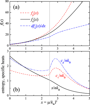
Figure 2. (a) 2D universal scaling functions fp
(x), fn
(x) and  as a function of the dimensionless variable
  . (b) 2D entropy
  and specific heats per particle
  and
and  , as a function of
  . The vertical grey lines indicate the critical threshold for superfluidity,
  [37].
[37].
Download figure:
Standard image High-resolution image2.4. Superfluid density
We can also express the local superfluid density as a universal (but as yet undetermined) function  :
:

Integrating out the axial coordinate, we obtain
where the universal scaling function fs (x) is given by

As mentioned earlier, in contrast to the equation of state, the universal function for the superfluid density of a unitary Fermi gas  is not yet known precisely [20, 29, 30]. For illustrative purposes in the present work, we will consider the superfluid fraction of superfluid helium [47],

which is plotted in figure 3 by red circles. Our choice is motivated by the similarity for hydrodynamics between superfluid helium and unitary Fermi gas, presumably arising from strong correlations in both systems, and justified in part by measurements in [28]. Using equation (6), we find that ![$T/{{T}_{{\rm c}}}={{[f_{n}^{3{\rm D}}(x)/f_{n}^{3{\rm D}}({{x}_{{\rm c}}}\simeq 2.49)]}^{-2/3}}$](https://content.cld.iop.org/journals/1367-2630/16/8/083023/revision1/njp499274ieqn42.gif) . Thus, from equation (27), the universal function
. Thus, from equation (27), the universal function  can be calculated using

and fs (x) is then obtained. In the inset of figure 3, we show fs (x) calculated with the superfluid fraction of superfluid helium.
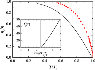
Figure 3. Bulk superfluid fraction of superfluid helium (red circles) [47] and the corresponding 2D reduced superfluid fraction (the black line). The inset shows the 2D universal scaling function for superfluid density, to be used for a unitary Fermi gas. The vertical grey lines indicate the critical threshold for superfluidity,  [37].
[37].
Download figure:
Standard image High-resolution imageIn a 2D configuration with  , it is natural to define a Fermi temperature in terms of the column density n2:
which coincides with the usual 3D definition of the Fermi temperature, equation (4). The reduced temperature is then given by,

Therefore, the critical temperature of the unitary Fermi gas in the pancake geometry is given by, ![$T_{{\rm c}}^{2{\rm D}}={{[2{{f}_{n}}({{x}_{{\rm c}}})/\sqrt{\pi }]}^{-1/2}}T_{{\rm F}}^{2{\rm D}}\simeq 0.198T_{{\rm F}}^{2{\rm D}}$](https://content.cld.iop.org/journals/1367-2630/16/8/083023/revision1/njp499274ieqn46.gif) . In figure 3, we show the 2D superfluid fraction
. In figure 3, we show the 2D superfluid fraction  (the black line) as a function of
  . It lies systematically below the 3D superfluid fraction (red circles), due to the integration over the axial degree of freedom.
It should be noted that the critical behavior of the superfluid density near the phase transition is greatly affected by the axial integration. In three dimensions, we may define the critical exponent α by  or
or  . After integrating out the axial degree of freedom, it is easy to show,

As we shall see, the increase in the critical exponent will reduce the second sound velocity and hence the second sound mode frequency.
3. 2D simplified two-fluid hydrodynamic equations
We now derive the simplified 2D Landau two-fluid hydrodynamic equations, following the idea by Bertaina, Pitaevskii and Stringari [24]. This 2D picture will generally be valid as we are considering excitations whose wavelength is long compared to the transverse (axial) cloud width.
The standard two-fluid equations in the harmonic trap Vext are given by,


where  is the current density, ns
and nn
are the superfluid and normal density,
is the current density, ns
and nn
are the superfluid and normal density,  and
and  are the corresponding velocity fields,
  , and finally η and κ are the shear viscosity and thermal conductivity, respectively. In the above equations, we have kept only linear terms in the velocity, as we are interested in small-amplitude dynamics in the linear response regime. Moreover, we have omitted bulk viscosity terms which give smaller contributions. The Landau two-fluid hydrodynamic theory is applicable when the mean free path l is much smaller than the wavelength of the sound wave λ. By considering the axial size of the Fermi cloud
  , we further require
  , therefore the hydrodynamic regime in a harmonic trap is achieved when
  .
.
As discussed by Stringari and co-workers [24], in the presence of tight confinement, the nonzero viscosity and thermal conductivity may significantly change the low-energy dynamics at the frequency  . This occurs when the viscous penetration depth δ—the typical length scale at which an excitation becomes damped due to shear viscosity—fulfils the condition

In the case of superfluid helium in a thin capillary, the above condition makes the normal component of the liquid stick to the wall and thus the normal velocity field vanishes [48]. With a soft wall caused by the tight axial confinement, the normal component can move but the normal velocity field becomes uniform along the axial direction [24]. For the same reason, the superfluid velocity also becomes independent of the axial coordinate. Analogously, a nonzero thermal conductivity in equation (35) for the entropy conservation leads to the independence of the temperature fluctuation  on the axial coordinate. The tight axial confinement also implies that the axial component of the velocity fields, for both superfluid and normal fluid, must be much smaller than the transverse one and may be neglected. Using equation (33) for the superfluid velocity implies that the chemical potential fluctuation
  is essentially independent of the axial coordinate. In brief, we conclude that, owing to the crucial roles played by the shear viscosity and thermal conductivity, under the tight axial confinement the velocity fields are independent of the axial position and a global thermal equilibrium along the axial direction is established.
With these observations, it is straightforward to write down the simplified two-fluid hydrodynamic equations by integrating out the axial degree of freedom in equations (32)–(34) and (35), which take the following forms,


where the current density now becomes  and we have omitted the residual dissipation terms along the weakly confined direction, as in a uniform fluid the effect of viscosity and thermal conductivity is irrelevant in the long-wavelength limit.
We note that, by introducing a characteristic collisional time τ related to viscosity,  , where
  is the average velocity of atoms and is of the order of the Fermi velocity
  , it is easy to check that equation (36) is equivalent to requiring the low frequency condition,

Recalling that  and
and  , the above requirement for achieving the reduced 2D hydrodynamics can be rewritten as
  . For a highly oblate trap with typical aspect ratio
  , this condition is compatible with the condition to enter the hydrodynamic regime,
  , which can alternatively be written as
  .
.
3.1. Variational reformulation of the simplified Landau hydrodynamic equations
A convenient way to solve the simplified two-fluid hydrodynamic equations is to reformulate them using Hamiltonʼs variational principle [49]. Following previous work [18, 20], the hydrodynamic modes of these equations with frequency ω at temperature T can be obtained by minimizing a variational action, which, in terms of displacement fields  and
and  ,1
takes the following form,
,1
takes the following form,
Here,  and
and  are the 2D reduced superfluid and normal-fluid densities at equilibrium, as discussed in the previous section section 2. The density fluctuation
  and entropy fluctuation
  are given by

and

respectively. The effect of the weak radial trapping potential  enters the action equation (42) through the coordinate dependence of the equilibrium thermodynamic variables
  ,
,  and
and  , within the local density approximation. We stress that, all these thermodynamic variables can be obtained by using the reduced Gibbs–Duhem relation equation (13) and can be expressed by the universal functions fp
(x) and fn
(x).
, within the local density approximation. We stress that, all these thermodynamic variables can be obtained by using the reduced Gibbs–Duhem relation equation (13) and can be expressed by the universal functions fp
(x) and fn
(x).
In superfluid helium, the solutions of the Landau two-fluid hydrodynamic equations can be well understood as density and entropy (temperature) waves, which are the pure in-phase mode with  and the pure out-of-phase mode with
  , known as first and second sound, respectively [2–4]. For a strongly interacting unitary Fermi gas, we could use the same classification [21]. For this purpose, we rewrite the action equation (42) in terms of two new displacement fields

and

considering that the density and temperature fluctuations are given by

and
respectively. Ideally, first sound is characterized by  but
but  and second sound by
  but
but  .
.
Using the standard thermodynamic identities derived from the reduced Gibbs–Duhem relation equation (13), after some straightforward but lengthy algebra, we arrive at

where
It is clear that the first and second sound are governed by the actions  and
and  , respectively. The coupling between first and second sound is controlled by the coupling term
  , which is in general nonzero. Indeed, in our case, as
  , strictly speaking the first and second sound are coupled at any finite temperatures.
4. Free-propagating first and second sound
For a uniform superfluid ( ), the solutions of
  and
and  are plane waves of wave vector q with dispersion
  and
and  , where
and
These expressions for first and second sound velocities are the standard results used to describe superfluid helium, when the corresponding equation of state and superfluid density are used [2–4]. In figure 4, we show the decoupled first and second sound velocities of a highly oblate Fermi gas at unitarity, by using dashed lines.
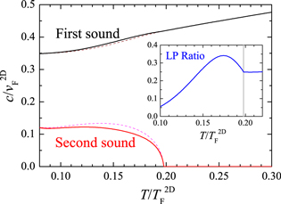
Figure 4. 2D first and second sound velocities (solid lines) as a function of temperature, in units of the Fermi velocity  of an ideal Fermi gas at zero temperature at the trap center. The dashed lines give the decoupled sound velocities. The inset shows the Landau–Placzek parameter
  . The vertical grey lines indicate the critical temperature for superfluidity,
  , in the absence of harmonic confinement in the transverse direction.
Download figure:
Standard image High-resolution imageIncluding the coupling term  and using the standard thermodynamic relations, it is straightforward to show that the solutions for sound velocities u of the simplified two-fluid hydrodynamic equations satisfy the following equation

where
It gives rise to two solutions for the sound velocity, u1 and u2, which in the absence of the coupling term  (i.e.,
  ), coincide with the decoupled first and second sound velocities, c1 and c2. The numerical results for u1 and u2 are shown in figure 4 by solid lines. The temperature dependence of the reduced sound velocities in figure 4 is very similar to that of a 3D unitary Fermi gas predicted in the earlier works [23, 29]. We attribute this qualitative similarity to the strongly interacting nature of the system.
In the case of a small parameter  , which is indeed true for a highly oblate unitary Fermi gas, we may solve equation (55) perturbatively. We find the expansions [23],


To the leading order of θ, the first sound velocity is not affected by the coupling term, but the second sound velocity decreases by a factor of  and is now given by [23, 26],

Therefore, quantitatively, the coupling between first and second sound can be characterized by the so-called Landau–Placzek (LP) parameter  [23]. In the inset of figure 4, we plot the LP parameter as a function of temperature. In the superfluid phase, it is always smaller than 0.4, indicating that the first and second sound couple very weakly in a unitary Fermi gas. A similar situation happens in superfluid helium, where
  and hence
  [20]. From the above approximate expression for the second sound velocity and equation (31) for 2D superfluid density, it is clear the velocity vanishes as
when approaching to the superfluid phase transition from below. Here,  is the critical exponent of the superfluid density of a unitary Fermi gas in three dimensions.
Although the coupling between first and second sound is weak in a unitary Fermi gas, it is of significant importance for the purpose of experimental detection of second sound. Unlike superfluid helium, temperature oscillations—the characteristic motion of the second sound—are difficult to observe in ultracold atomic gases. Density measurement is the most efficient way to characterize any low-energy dynamics. As a result, an observable second sound mode must have a sizable density fluctuation, which can only be induced by its coupling to first sound modes. The strength of density fluctuations in second sound may be conveniently characterized by the following ratio between the relative density and temperature fluctuations,
where the subscript ‘2nd’ indicates the second sound and we have taken the derivative at const pressure, as the second sound is properly considered as an oscillating wave at constant pressure, rather than at constant density, as indicated by equation (59) [26]. In contrast, the ratio between the relative density and temperature fluctuations in first sound is given by

In figure 5, we report the density fluctuation of second sound as a function of temperature in the superfluid phase, calculated with an assumed temperature fluctuation ratio  . This is a typical temperature fluctuation, achievable in current experiments. For example, in the recent first-sound collective mode measurement, it was shown that
  over a wide temperature window [16, 17]. By using equation (62), we therefore assume that a temperature fluctuation at
  can be easily excited. From figure 5, it is easy to see that the density fluctuation of second sound is very significant when temperature
  , revealing that the propagation of a second sound pulse could be experimentally detected via density measurements. This result suggests that a similar approach to that demonstrated by the Innsbruck experiment [28] could be applied in the oblate geometry considered here, where a focused blue-detuned laser propagating along the tightly confined direction could excite a second sound wave which will propagate radially outwards from the cloud centre. Subsequent absorption images taken at different times after the laser pulse could record the density fluctuation induced by the propagating second sound wave.
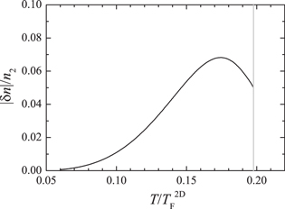
Figure 5. The density fluctuation of 2D second sound, calculated in the case of  . The vertical grey lines indicate the critical temperature for superfluidity,
  , in the absence of harmonic confinement in the transverse direction.
Download figure:
Standard image High-resolution imageWhile the essential physics of our scheme is the same as that considered by by Stringari and co-workers in highly elongated trap [26], the quasi-2D geometry may offer advantages for experiments. Specifically, clouds confined in elongated traps typically have very high peak densities leading to high optical densities that are difficult to measure quantitatively using absorption imaging [50, 51]. This means quantifying small density fluctuations in such clouds can prove challenging. In a quasi-2D trap however, such high peak optical densities can be avoided and images taken along the direction of tight confinement can be integrated over the angular coordinate to obtain an accurate measure of the radial density. Small density fluctuations should therefore be more easily detected.
5. Breathing first and second sound modes in harmonic traps
We now consider a weak transverse harmonic trap,  and fully solve the simplified Landau two-fluid hydrodynamic equations using a variational approach, developed in the previous work [20, 21]. We focus on compressional (breathing) modes with the projected angular momentum
  , since these modes are the easiest one to excite experimentally.
5.1. Variational approach
For breathing modes, we assume the following polynomial ansatz for the displacement fields:

where  is the unit vector in the radial direction,
  (
( ) are the 2Np
variational parameters, and
) are the 2Np
variational parameters, and  is the dimensionless radial coordinate with RF being the Thomas–Fermi radius. By inserting this variational ansatz into the action equation (49), we express the action S as functions of the 2Np
variational parameters
is the dimensionless radial coordinate with RF being the Thomas–Fermi radius. By inserting this variational ansatz into the action equation (49), we express the action S as functions of the 2Np
variational parameters  . The mode frequencies are obtained by minimizing the action S with respect to these 2Np
parameters. The accuracy of our variational calculations can be improved by increasing the value of Np
. It turns out that the calculations converge quickly as Np
increases.
. The mode frequencies are obtained by minimizing the action S with respect to these 2Np
parameters. The accuracy of our variational calculations can be improved by increasing the value of Np
. It turns out that the calculations converge quickly as Np
increases.
In more detail, it is straightforward to show that, the expression of the action can be written in a compact form

where ![$\Lambda \equiv {{\left[ {{A}_{0}},{{B}_{0}},\ldots ,{{A}_{i}},{{B}_{i}},\ldots ,{{A}_{{{N}_{p}}-1}},{{B}_{{{N}_{p}}-1}} \right]}^{T}}$](https://content.cld.iop.org/journals/1367-2630/16/8/083023/revision1/njp499274ieqn125.gif) and
and  is a
is a  matrix with block elements (
 ),
),
In ![${{[\mathcal{S}\left( \omega \right)]}_{ij}}$](https://content.cld.iop.org/journals/1367-2630/16/8/083023/revision1/njp499274ieqn129.gif) , we have introduced the weighted mass moments,
, we have introduced the weighted mass moments,


and the spring constants,


To derive the above equations, we have used the universal relations satisfied by the highly oblate unitary Fermi gas:  and
and  . Moreover, we have used integration by parts to simplify the expressions: for example, the contributions from the middle two terms in equation (50) with
  can be shown to cancel with each other with our polynomial ansatz. For a given value of
  (or
(or  , see equation (12)), the weighted mass moments and spring constants can be calculated by using local thermodynamic variables in equations (14), (17), (18), (20) and (25). The detailed expressions for numerical calculations are listed in appendix
It is easy to see that the minimization of the action S is equivalent to solving

or  . The detailed numerical procedure is presented in appendix
We have performed numerical calculations for the number of the variational parameter Np
up to ten, for any given chemical potential  or temperature
  . In the following, we first discuss the decoupled first and second sound. Then, we focus on the effect of the coupling between first and second sound and the density fluctuation of second sound modes.
5.2. Decoupled first and second sound
In figures 6(a) and (b), we present mode frequencies of decoupled first and second sound modes of a highly oblate unitary Fermi gas, obtained by solving the individual action  and
and  , respectively.
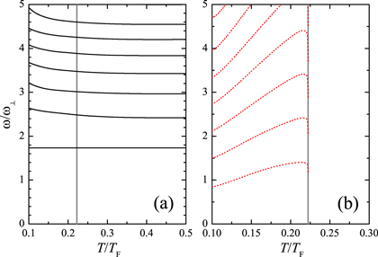
Figure 6. The mode frequencies of decoupled first (a) and second sound (b). The vertical grey lines show the critical temperature of a three-dimensional trapped unitary Fermi gas,  .
.
Download figure:
Standard image High-resolution imageFor all the first sound modes, except the lowest-lying one, the mode frequency decreases monotonically with increasing temperature, exhibiting the same temperature dependence as the first sound modes in an isotropic [21] or highly elongated harmonic trap [16, 26]. The lowest-lying breathing mode instead does not depend on the temperature and takes an invariant mode frequency  . We note that such a temperature independence is a peculiarity of the unitary Fermi gas due to its inherent scale invariance. Indeed, our variational ansatz
  of the lowest-lying breathing mode is one of the few exact scaling solutions exhibited by the Landau two-fluid hydrodynamic equations at unitarity [25]. To understand this, we simply recall that the spring constant
  satisfies

Thus, if i = 0 or j = 0, we have  . Taking into account the fact that
  or
or  , it is readily seen from equation (66) that
  provides an exact solution, regardless the number of the variational ansatz used. We note also that, the first sound solutions converge very quickly with the number of the variational parameters, indicating that these solutions are indeed well-approximated by the polynomial function.
For second sound modes, we find that the mode frequency initially increases with increasing temperature and then drops to zero very dramatically when the temperature approaches to the critical value. This behavior differs from the earlier result in a 3D isotropic harmonic trap [21] but agrees with a recent prediction made for a high elongated configuration [26]. Qualitatively, we may estimate the discretized second sound mode frequency by using the expression  with a characteristic wavevector
  , where Rs is the size of the superfluid component along the radial direction. Within the local density approximation, we have
  . Using equation (60)
  , we obtain that
Thus, for the critical exponent  , the second sound mode frequency ω vanishes at Tc. The superfluid density data (i.e., of superfluid helium) that we use have a critical exponent
  , and consequently, we find the vanishing frequency at the transition.
5.3. Full solutions of 2D two-fluid hydrodynamics
We now include the coupling term  . In figure 7, we report the full variational results by blue circles. For comparison, the decoupled first and second sound mode frequencies are also shown, by black lines and red dashed lines, respectively. As anticipated, the exact solution with frequency
  remains unchanged with the inclusion of the coupling term.
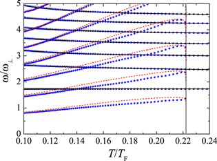
Figure 7. Temperature dependence of the full two-fluid hydrodynamic mode frequencies (blue circles). For comparison, we show also the mode frequencies of decoupled first and second sound, respectively, by black solid and red dashed lines. The vertical grey lines show the critical temperature of a three-dimensional trapped unitary Fermi gas,  .
.
Download figure:
Standard image High-resolution imageVery similar to the sound velocities in the uniform case (see figure 4), the first sound mode frequency is barely affected by the coupling term  . This is particularly evident in figure 8(a), in which we show an enlarged view for the n = 2 first sound mode (the integer n labels the nth first sound modes). The correction to the first sound mode frequency due to the coupling is about
  and occurs only at around
  .
.
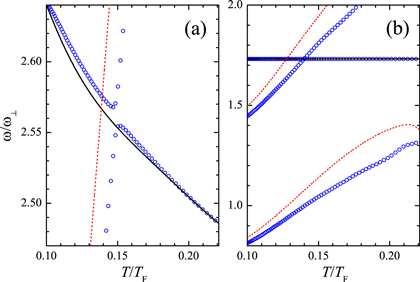
Figure 8. Enlarged view of the full two-fluid hydrodynamic mode frequencies (blue circles), near the n = 2 first sound mode (a) and the lowest two second sound modes (b). In the left panel, the avoided crossing between first and second sound is evident.
Download figure:
Standard image High-resolution imageOn the other hand, the frequency of second sound modes is notably pushed down by the coupling term  , as can be seen from figure 8(b). The maximum correction is up to 20% when the temperature is about
  . In the uniform case, i.e., figure 4, we find a similar correction to the second sound velocity in the same temperature regime.
5.4. Density fluctuations of sound modes
The sizable correction in the mode frequency of a second sound mode strongly indicates that, its density fluctuation, as a result of the coupling to first sound modes, should also be significant. In figure 9(b), we show the density fluctuations of the lowest two first sound modes (m = 2 and 4) and of the lowest two second sound modes (m = 1 and 3), at a temperature  . Here, we have used the integer m as the index of different modes when the coupling term is taken into account.
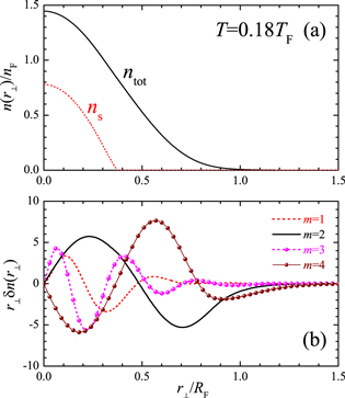
Figure 9. (a) Density distribution (the black line) and superfluid density distribution (the red dashed line) at  , in units of the peak linear density of an ideal Fermi gas at zero temperature and at the trap center (nF). (b) Density fluctuations (in arbitrary unit) of the lowest two first-sound (solid lines) and second-sound modes (dashed lines).
Download figure:
Standard image High-resolution imageRemarkably, the amplitude of the second sound density fluctuations is just a bit smaller than that of the first sound modes, over a wide range of temperatures, revealing that it could be detected experimentally. In this respect, we note that, most recently the density fluctuations of the low-lying first sound modes have been measured in a highly elongated unitary Fermi gas, to a reasonably good precision [16]. Therefore, it is very likely that a low-lying second sound mode could also be observed by looking at its density fluctuation, after proper excitation.
Comparing the density and superfluid density profiles, shown in figure 9(a), we find that the density fluctuation of second sounds is most significant within the superfluid core, in accordance with their temperature-wave nature. In contrast, the density fluctuation of first sound modes extends over the whole Fermi cloud.
5.5. Dependence on the superfluid density
We not that, a complete theoretical description of the superfluid density for a Fermi gas at unitarity is yet to be determined due to the theoretical difficulties in handling the strong interaction. In the above studies, we have considered the superfluid fraction of superfluid helium for the superfluid density of the unitary Fermi gas, see, for example, equations (27) and (28). As the second sound is arguably the most significant demonstration of superfluid, it is natural to anticipate that the mode frequency of second sound modes should depend very sensitively on the form of superfluid density.
We have performed numerical calculations with other models of the superfluid density, as shown in figure 10. The two additional models we considered are: firstly,  , which is in magnitude similar to the superfluid fraction of superfluid helium but with a mean-field-like critical exponent
  ; secondly,
  , which differs significantly from the superfluid fraction of superfluid helium but takes into account the correct critical exponent
  . The predicted mode frequencies for different superfluid density are shown in figure 11.
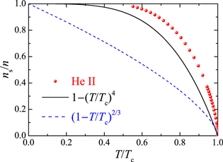
Figure 10. Bulk superfluid fraction: the black line and blue dashed line correspond to the choices,  and
and  , respectively. The red circles are the superfluid fraction of superfluid helium [47]. Note that, recently the superfluid fraction of a 3D unitary Fermi gas has been calculated by Salasnich based on the Landauʼs expression for superfluid density and physical elementary excitations [29]. The predicted temperature dependence is similar to what we have shown in the figure, presumably due to the simialr elementary excitations arising from strong interactions.
Download figure:
Standard image High-resolution image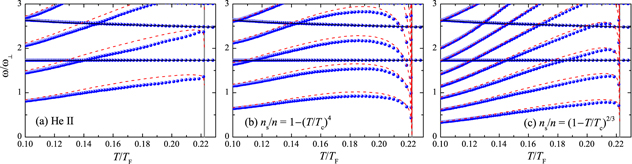
Figure 11. Sensitivity of second sound modes on the bulk superfluid density. The vertical grey lines show the critical temperature of a three-dimensional trapped unitary Fermi gas,  .
.
Download figure:
Standard image High-resolution imageIt is readily seen that the mode frequency of second sound modes displays a very sensitive dependence on both the magnitude and critical exponent of the superfluid density. In particular, the mode frequency with the superfluid-helium-like superfluid fraction (figure 11(a)) differs significantly from that with the choice  , although these two superfluid fractions differ slightly in magnitude. The strong dependence is very encouraging, indicating that practically, the superfluid density of a unitary Fermi gas could be accurately determined by measuring the mode frequency of low-lying second sound modes.
5.6. Experimental considerations
Ideally, a compressional second sound mode would be excited by modulating the trapping frequency close to the predicted mode frequency. However, in our quasi-2D configuration, this can be problematic due to the fact that the radial confinement is generated by a magnetic field, whose modulation can also change the s-wave scattering length and hence the system may be away from the unitary regime. We note that this problem does not exist in other setups where it is possible to have optical radial (and axial) confinement.
For our experimental setup at Swinburne, therefore, a more practical scheme would be to locally perturb the cloud and allow it to relax. Taking inspiration from the selective excitation schemes, developed by the Innsbruck experiments [17], one may direct an appropriately sized blue-detuned laser beam into the cloud and apply a modulation burst, chosen to provide the best mode matching with the calculated second sound mode. The power, duration and shape of the laser beam should be optimized in order to resonantly derive the desired small amplitude oscillation in the linear response regime.
6. Conclusions
In conclusion, we have derived the 2D simplified Landau two-fluid hydrodynamic equations to describe the low-energy dynamics of a unitary Fermi gas confined in highly oblate harmonic traps. By using a variational approach, these two-fluid hydrodynamic equations have been fully solved. We have discussed in detail the resulting density-wave (firsts sound) and temperature-wave (second sound) oscillations, in the absence or presence of a weak transverse harmonic trap. First and second sound velocities or discretized mode frequencies have been predicted, accordingly.
We have found a weak coupling between first and second sound in highly oblate unitary Fermi gas, very similar to the case of superfluid helium. Though the coupling is weak, it induces significant density fluctuations for second sound modes, indicating that second sound could be potentially observed in the highly oblate configuration, by measuring the density fluctuations. Owing to the strong sensitivity of second sound mode frequencies to superfluid density, the experimental measurement of discretized second sound modes could provide a promising way of accurately determining the superfluid density of a unitary Fermi gas.
Acknowledgements
We thank Martin W Zwierlein and Mark J-H Ku for providing us their experimental data. This research was supported by the ARC Discovery Projects Grant nos. FT130100815 (HH), DP140103231 (HH), DE140100647 (PD), FT120100034(CJV), DP130101807 (CJV) and DP140100637 (XJL), and NFRP-China Grant no. 2011CB921502 (XJL, HH).
Appendix A.: Equation of state of a unitary Fermi gas
In the low temperature superfluid phase, we fit the experimental data of g(x) by using the Pad approximant of order [2/2],
where  is the Bertsch parameter [37], and obtain
  ,
,  ,
,  and
and  .
.
For the normal state, i.e., ![$x\subset [-1.2,{{x}_{{\rm c}}}\simeq 2.49]$](https://content.cld.iop.org/journals/1367-2630/16/8/083023/revision1/njp499274ieqn177.gif) , we fit the data with a fourth order polynomial
, we fit the data with a fourth order polynomial

and find that  ,
,  ,
,  ,
,  and
and  . At high temperatures where
  , we use the virial expansion form,

where  and
and  are the second and third virial coefficients of a unitary Fermi gas [45, 46], respectively. To make g(x) smooth across the whole normal state, we connect
  and
and  by using the expression,

Recalling that  at
at  , we therefore set
  . We note that, we do not need to impose the constraint
  , due to the superfluid phase transition.
Appendix B.: Matrix elements of 

In this appendix, we present the weighted mass moments and spring constants in their dimensionless form,
and
respectively, for the purpose of performing numerical calculations. Accordingly, we solve the matrix  in its dimensionless form,
where  is the reduced frequency. For given chemical potential
  or temperature
  , these dimensionless matrix elements are given by, after taking
  ,
,


for the weighted mass moments and


for the spring constants. In the above expressions, the argument for the universal scaling functions is  , i.e.,
 ![$[{{f}_{n}}]$](https://content.cld.iop.org/journals/1367-2630/16/8/083023/revision1/njp499274ieqn199.gif) is the short-hand notation of
is the short-hand notation of ![${{f}_{n}}[{{\mu }_{0}}/({{k}_{{\rm B}}}T)-y/(T/{{T}_{{\rm F}}})]$](https://content.cld.iop.org/journals/1367-2630/16/8/083023/revision1/njp499274ieqn200.gif) , and
, and  stands for the derivative
 /{\rm d}x.$](https://content.cld.iop.org/journals/1367-2630/16/8/083023/revision1/njp499274ieqn202.gif)
Appendix C.: Solving
![${\rm det} [\tilde{S}(\tilde{\omega })]=0$](https://content.cld.iop.org/journals/1367-2630/16/8/083023/revision1/njp499274ieqn203.gif)
To solve the matrix equation

where the vector of displacement fields, ![$\Lambda ={{[{{A}_{0}},{{B}_{0}}...,{{A}_{i}},{{B}_{i}},...]}^{T}}$](https://content.cld.iop.org/journals/1367-2630/16/8/083023/revision1/njp499274ieqn204.gif) , we rewrite the matrix
, we rewrite the matrix  . Here,
  and
and  denote collectively the matrix of the dimensionless weighted mass moments and the spring constants, respectively. The matrix
  is positively definite, so that we decouple it by a product of a lower triangular matrix
  and its transpose,

In terms of this decomposition, the matrix equation, equation (C.1), becomes

It is easy to see that the matrix ![$[{{{\bf L}}^{-1}}\cdot {\bf K}\cdot {{({{{\bf L}}^{-1}})}^{T}}]$](https://content.cld.iop.org/journals/1367-2630/16/8/083023/revision1/njp499274ieqn210.gif) is symmetric and its eigenvalues give rise to the desired solution of mode frequencies. The displacement field for each eigenvalue can also be calculated accordingly, with known eigenstate of the matrix
is symmetric and its eigenvalues give rise to the desired solution of mode frequencies. The displacement field for each eigenvalue can also be calculated accordingly, with known eigenstate of the matrix ![$[{{{\bf L}}^{-1}}\cdot {\bf K}\cdot {{({{{\bf L}}^{-1}})}^{T}}]$](https://content.cld.iop.org/journals/1367-2630/16/8/083023/revision1/njp499274ieqn211.gif) . More explicitly, if we denote an eigenstate by
. More explicitly, if we denote an eigenstate by  , the corresponding displacement field is given by

Once the displacement fields for a mode are found, we may calculate its density fluctuation and temperature fluctuation.
Footnotes
- 1
In the time domain, the displacement fields
and are defined by, and