Abstract
The bacterial genome is organized by a variety of associated proteins inside a structure called the nucleoid. These proteins can form complexes on DNA that play a central role in various biological processes, including chromosome segregation. A prominent example is the large ParB-DNA complex, which forms an essential component of the segregation machinery in many bacteria. ChIP-Seq experiments show that ParB proteins localize around centromere-like parS sites on the DNA to which ParB binds specifically, and spreads from there over large sections of the chromosome. Recent theoretical and experimental studies suggest that DNA-bound ParB proteins can interact with each other to condense into a coherent 3D complex on the DNA. However, the structural organization of this protein-DNA complex remains unclear, and a predictive quantitative theory for the distribution of ParB proteins on DNA is lacking. Here, we propose the looping and clustering model, which employs a statistical physics approach to describe protein-DNA complexes. The looping and clustering model accounts for the extrusion of DNA loops from a cluster of interacting DNA-bound proteins that is organized around a single high-affinity binding site. Conceptually, the structure of the protein-DNA complex is determined by a competition between attractive protein interactions and loop closure entropy of this protein-DNA cluster on the one hand, and the positional entropy for placing loops within the cluster on the other. Indeed, we show that the protein interaction strength determines the ‘tightness’ of the loopy protein-DNA complex. Thus, our model provides a theoretical framework for quantitatively computing the binding profiles of ParB-like proteins around a cognate (parS) binding site.
Original content from this work may be used under the terms of the Creative Commons Attribution 3.0 licence. Any further distribution of this work must maintain attribution to the author(s) and the title of the work, journal citation and DOI.
1. Introduction
Understanding the biophysical principles that govern chromosome structure in both eukaryotic and prokaryotic cells remains an outstanding challenge [1–7]. Many bacteria have a single chromosome with a length three orders of magnitude longer than the cell itself, posing a daunting organizational problem. Owing to recent technological advances in live-cell imaging and chromosome conformation capture based approaches, it is becoming increasingly clear that the DNA is not coiled like a simple amorphous polymer inside the cell [8–10], but rather exhibits a high degree of organization over a broad range of lengthscales [11]. It remains unclear, however, how this spatial and dynamic organization of the chromosome is established and maintained inside living bacteria [12]. A host of nucleoid-associated proteins (NAPs) have been shown to play a central role in the spatial organization of the bacterial chromosome [12–14]. Such NAPs bind to the DNA in large numbers, and by interacting with each other and with DNA in both sequence-dependent and sequence-independent manners they can collectively structure the DNA polymer and control chromosome organization, e.g. by DNA looping. More generally, the formation of loops appears to play a fundamental role in structuring DNA in both bacterial DNA and eukaryotic chromatin and further theoretical and simulation studies are needed to clarify the mechanisms at play [15, 16].
In many bacterial species, the broadly conserved ParABS system is responsible for chromosome and plasmid segregation [12, 17]. A central component of this system is the partitioning module, which is formed by a large protein-DNA complex of ParB proteins that assembles around centromere-like parS sites, frequently located near the origin of replication. The ParBS complexes can subsequently interact with ParA ATPases, leading to the segregation of replicated origins [18–25]. How is this ParBS partitioning module physically organized on the DNA? ParB is known to bind specifically to parS, triggering the formation of a large protein-DNA cluster, which is visible as a tight focus in microscopy images of fluorescently labeled ParB [17, 21, 26, 27]. The propensity of ParB to form foci around parS has been exploited in recent studies, which used exogenous expression of fluorescently labeled ParB along with parS insertion to label DNA loci for live-cell imaging [28, 29]. In the F-plasmid of Escherichia coli cells, each ParB focus contains roughly 300 proteins, together representing 90% of all ParB present in the cell [27]. High-precision ChIP-Seq experiments on this system provide quantitative ParB binding profiles along the DNA, which are strongly peaked around parS with a broad decay over a distance of up to 13 kilobasepairs (kb), consistent with earlier observations [26, 30].
Various models have been introduced to explain the distribution of ParB along DNA around parS sites. An early study of the distribution of ParB proposed that ParB proteins spread from the parS sequence by nearest-neighbor interactions, forming a continuous filament-like structure along the DNA [30]. This model was termed the spreading model. However, this is effectively a 1D model with short range interactions. On general statistical physical grounds, such a 1D model cannot be expected to account for the formation of a large coherent protein-DNA complex, given physiological protein interaction strengths [31]. Furthermore, the number of ParB proteins available in the cell is not sufficient to allow enrichment by simple 1D polymerization of ParB along DNA at genomic distances from parS as large as observed experimentally [27]. To resolve the puzzle of how ParB proteins organize around a parS site, we recently introduced a novel theoretical framework to study the collective behavior of interacting proteins that can bind to a DNA polymer [31]. This model suggested that ParB assembles into a three-dimensional complex on the DNA, as illustrated in figures 1(a) and (b). Single molecule experiments provided direct evidence for the presence of 3D bridging interactions between two ParB proteins on DNA [32, 33]. We showed that a combination of such a 3D bridging bond and 1D spreading bonds between ParB proteins constitutes a minimal model for the condensation of ParB proteins on DNA into a coherent complex [31], consistent with the observation that ParB-GFP fusion proteins form a tight fluorescent focus on the DNA [17, 21, 26, 27].
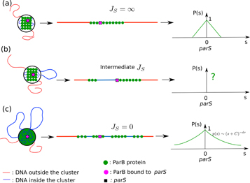
Figure 1. Schematic illustration of two recent models proposed to describe the ParB partition complex (left) accompanied by a typical distribution of ParB on extended DNA (middle), and the average distribution profile (right). The spreading and bridging model [31] is shown with (a) strong coupling  , where thermal fluctuations cannot break the bonds between proteins such that all bridging and spreading interactions are satisfied, and (b) intermediate coupling where the energetic cost of breaking a spreading bond combined with the cost in loop closure entropy competes with the positional entropy of placing loops within the cluster. With the looping and clustering approach presented here, we propose a simple analytic description for this regime. (c) The stochastic binding model assumes a spherical region of high concentration of ParB around parS [27]. This model can be seen as taking the limit of the spreading bond strength to zero (
 ), and thus the formation of loops is not hampered by protein–protein bonds. In this limit, the binding profile can be described as the return of the polymer to an origin of finite size, such that the profile is given by
  , where d is the dimension, ν is the Flory exponent, and C is a constant.
Download figure:
Standard image High-resolution imageThe statistical properties of the 3D structure of ParB-DNA complexes determines the binding profile of ParB on DNA, which can be accurately measured in ChIP-Seq experiments. However, it is computationally demanding to simulate these binding profiles with the spreading and bridging model. The protein binding profiles can be easily calculated analytically in the limit of strong protein–protein interactions, where the cluster of ParB on the DNA becomes compact with a corresponding triangular distribution of ParB along DNA. The protein binding profiles can also be estimated in the limit of weak protein–protein interactions with the so-called stochastic binding model, where a sphere of high ParB concentration is assumed to exist within which a DNA polymer freely fluctuates [27] (see figure 1(c)). The description of the average protein binding profile is thus similar to the return statistics of the polymer into the ParB sphere [34], suggesting a long range (power-law) distribution of ParB proteins along DNA. Importantly, however, neither of these two existing approaches provide a simple way of computing ParB binding profiles around parS sites over the full relevant range of system parameters. In addition, it remains unclear how the spreading and bridging model and the stochastic binding model relate to each other.
Here, we propose a theoretical approach to describe the distribution of ParB proteins around parS sites on the DNA in terms of molecular interaction parameters and protein expression levels. To this end, we develop a simple model for protein-DNA clusters that explicitly accounts for the competition between the positional entropy associated with placing the loops on the cluster, which favors a looser cluster configuration, and both protein–protein interactions and loop closure entropy, which tend to favor a compact cluster. This looping and clustering (LC) model represents a reduced, approximate version of the full spreading and bridging model that incorporates the key physical ingredients needed to provide a clearer understanding and at the same time greatly facilitates calculations of the distribution profile of ParB (or other proteins that form protein-DNA clusters). Thus, our approach can be used to estimate molecular interactions between proteins from experimentally determined protein binding profiles.
2. The looping and clustering (LC) model
To theoretically describe the protein binding profiles of ParB on DNA, we first consider a DNA polymer of length L that can move in space on a 3D cubic lattice and with a finite number of proteins m. Since the number of ParB proteins in the protein-DNA cluster has been observed to include the vast majority of proteins in the cell [27], we employ a canonical ensemble with a fixed number of ParB proteins m in the ParB complex. These proteins are able to diffuse along the DNA. Importantly, in this model the DNA itself is also dynamic and fluctuates between different three-dimensional configurations, which are affected by the presence of interacting DNA bound proteins. When proteins are bound to the DNA, they are assumed to be able to interact attractively with each other by contact interactions in two distinct ways: (i) 1D spreading interactions with coupling strength JS, defined as an interaction between proteins on nearest-neighbor sites along the polymer, and (ii) a 3D bridging interaction with strength JB between two proteins bound to sites on non-nearest neighbor-sites on the DNA, but which are positioned at nearest neighbor-sites in 3D space (see figures 1(a) and (b)). Thus, these bridging interactions couple to the 3D configuration of the DNA, while the 1D spreading interactions do not. Single-molecule experiments provide evidence for bridging bonds [32], with the bridging valency of a ParB protein limited to one [35, 36]. Even in this case where each protein can form two spreading bonds and a single bridging bond, the system has been shown to exhibit a condensation transition where the majority of the proteins form a single large cluster that can be localized by a single parS site on the DNA [31].
While it is possible to perform Monte Carlo simulations of the spreading and bridging model for a lattice polymer, such simulations are computationally demanding. In this paper, we aim to provide a simple analytical description for the average binding profile of proteins along the DNA (see right panels in figure 1). With this aim in mind, we can simplify our description by realizing that the configurations of ParB proteins along the DNA are more sensitive to JS than to JB, for sufficiently large JB. While both spreading and bridging bonds are necessary for the condensation of all proteins into a single cluster, loop extrusion from the cluster is controlled by JS, and such loop extrusion strongly impacts the binding profile of proteins on the DNA. Indeed, a loop can be extruded from the protein-DNA cluster by breaking a spreading bond, but without effecting the internal configuration of the bridging bonds. Therefore, we will assume that JB is sufficiently large to maintain a coherent 3D protein-DNA cluster, leaving JS as the main adjustable parameter in the model.
A contiguous 3D cluster of proteins on DNA with loops can effectively be represented graphically by a disconnected 1D cluster along the DNA, where connections in 3D between the 1D subclusters are implied, and domains of protein-free DNA within the disconnected 1D cluster represent loops that emanate from the 3D cluster (see figures 1(b) and (c)). We can describe this system by a reduced model for the effective 1D cluster in which we account for the entropy of the loops that originate from the protein-DNA cluster. In this model, the spreading bond energy set by the parameter JS combined with the cost in loop closure entropy, competes with the positional entropy for placing loops on the cluster and will therefore play a crucial role in determining the binding profile of ParB on DNA around a parS site.
To capture these effects, we propose the reduced LC model, which offers a simplified description of 3D protein-DNA clusters with spreading and bridging bonds. In this model a loop is formed whenever there is a gap between 1D clusters. We can make the connection between the gaps in the 1D cluster and the number of loops extending from the 3D cluster explicit by writing down the partition function for this model. The effective 1D cluster corresponding to a 3D cluster with m proteins and n loops has a multiplicity:

which counts the number of ways in which one can partition m proteins into n + 1 subclusters in 1D. This multiplicity leads to a positional entropy of mixing, Scluster = ln Ωcluster, for placing n loops at m − 1 possible positions (in units of kB). Note, we do not explicitly include the number of ways in which the bridging bonds can be formed, since loop formation is not expected to substantially affect the possible configurations of bridging bonds. However, creating n loops will require breaking n spreading bonds, and the probability at equilibrium for this to occur will include a Boltzmann factor  , where the interaction energy is expressed in units of kBT. Within our simple description, we do not consider how the formation of a loop affects the full internal entropy of the protein-DNA cluster, but this can be expected to be a fixed number per loop that can be absorbed into JS. Furthermore, the loops that are formed are assumed to be independent, and thus contribute to the loop closure entropy (in units of kB) as [34]:

where d is the spatial dimension, ν is the Flory exponent, and the loop length is measured in units of the lattice spacing of the polymer a, which we take to be equal to the footprint of a ParB protein, e.g. 16 bp for the exogenous ParABS system of E. coli [27].
This entropy is obtained by considering both the loops formed within the protein cluster and the protein-free segment of DNA outside the cluster. Indeed, the number of configurations associated with loop i for a Gaussian polymer is given by  [34, 37], where z is the lattice coordination number. Therefore, there is also an extensive contribution to the entropy given by kBℓi ln(z). However, when a loop of length ℓi forms, the same length of polymer is removed from the DNA outside of the cluster, which also results in a reduction of the entropy by kBℓi ln(z). Thus, there is a precise cancelation between the extensive contribution to the entropy associated with the loop inside the cluster and the extensive contribution due to effectively shortening the DNA outside the cluster5
.
[34, 37], where z is the lattice coordination number. Therefore, there is also an extensive contribution to the entropy given by kBℓi ln(z). However, when a loop of length ℓi forms, the same length of polymer is removed from the DNA outside of the cluster, which also results in a reduction of the entropy by kBℓi ln(z). Thus, there is a precise cancelation between the extensive contribution to the entropy associated with the loop inside the cluster and the extensive contribution due to effectively shortening the DNA outside the cluster5
.
It is now straightforward to write down the partition function of the LC model:

where ![${J}_{S}^{{\prime} }={J}_{S}+\mathrm{ln}[{{\ell }}_{0}^{d\nu -1}(d\nu -1)]\gt {J}_{S}$](https://content.cld.iop.org/journals/1367-2630/20/3/035002/revision2/njpaaad39ieqn6.gif) is a renormalized loop activation energy that includes the cost in loop closure entropy. All lengths are measured in units of the protein’s footprint a, ℓ0 is the lower cutoff of loop sizes and approximately represents the persistence length of DNA, and the bond interactions are in units of kBT. In the partition function, we conveniently set the upper boundary of integration, ℓmax, to infinity. Strictly speaking, the upper boundary for ℓj should be L − (m + Lj), where
is a renormalized loop activation energy that includes the cost in loop closure entropy. All lengths are measured in units of the protein’s footprint a, ℓ0 is the lower cutoff of loop sizes and approximately represents the persistence length of DNA, and the bond interactions are in units of kBT. In the partition function, we conveniently set the upper boundary of integration, ℓmax, to infinity. Strictly speaking, the upper boundary for ℓj should be L − (m + Lj), where  represents the total accumulated loop length before loop j. In practice, however, for chromosomes, but arguably also for plasmids, L ≫ m and the probability to have a large loop is very small. For instance, if we consider the F-plasmid of E. coli with a length of 60 kbp, we have L = 3750 in units of the ParB footprint of 16 bp [27, 38]. For this system, Monte Carlo (MC) simulations (see appendix A) of the LC model, with m = 100 reveal that the average cumulated loop size is ≈500 for small couplings (JS = 1) down to ≈25 for large couplings (JS = 4), which in both cases is much less than the DNA length. Thus, for biologically relevant cases it is reasonable to assume that the length of the DNA polymer is much larger than the footprint of the whole protein complex on the DNA.
The LC model constitutes a simple statistical mechanics approach to describe how proteins assemble into a protein-DNA cluster with multiple loops. Next, we will include a parS site on the DNA, to which ParB proteins bind with a higher affinity than the other non-specific binding sites on the DNA. Our central aim is to compute the binding profile of ParB around this parS site.
3. Profile of Par B for fixed number and sizes of loops
With our approach, we aim to quantitatively describe average ParB binding profiles, which are directly measurable by ChIP-Seq experiments. By fitting our model to such ChIP-Seq data, it would be possible to extract microscopic parameters such as the number of proteins in the ParB clusters and the protein–protein interaction parameters such as JS. In this section, we will describe how to compute the ParB binding profile around this parS site given a fixed number of loops with specified loop lengths. Then we will use the statistical mechanics framework provided above, to perform a weighted average over all possible loop numbers and sizes to arrive at a simple predictive theory for the ParB binding profile.
3.1. 1-loop binding profile
It is instructive to start our analysis of ParB binding profiles by first calculating the probability of ParB occupancy as a function of distance from the parS site for the case of a protein-DNA cluster with only one DNA loop (n = 1) with fixed loop length ℓ. We will assume a fixed number m of ParB proteins in this 1-loop protein-DNA cluster, and that one of these proteins is bound to the parS site at any time, as illustrated in figure 2. Thus, to calculate the 1-loop ParB binding probability, P1(s, ℓ), at a distance s from parS, we need to consider all possible configurations of proteins in the protein-DNA cluster subject to these constraints.
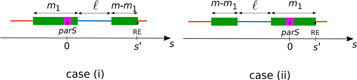
Figure 2. Schematic of the system with m proteins and a single loop of size ℓ. The whole cluster is split in two parts: m1 is the number of proteins in the cluster that overlaps with parS and m − m1 is the number of proteins in the other cluster. The origin of the genomic coordinates is parS, the right edge of the system (RE) is located at the coordinate  . We can divide the configurations into two equally likely cases: (i) the leftmost cluster overlaps with parS or (ii) the rightmost cluster overlaps with parS.
Download figure:
Standard image High-resolution imageFirst, we note that P1(s, ℓ) = 0 for s > m + ℓ, because the 1D cluster can maximally extend to a distance m + ℓ, which occurs when the 1D cluster adopts a configuration that lies entirely on one side of the parS site. For a binding site at a distance s < m + ℓ, the ParB binding probability is reduced, either by configurations where this site is located on the DNA loop within the 1D cluster, or by states where the 1D cluster adopts a configuration around the parS site that does not extend to the binding site at s, placing this site outside the 1D cluster. To capture these effects, it is helpful to express P1(s, ℓ) in terms of conditional probabilities:

where ‘loop(s)’ represents a condition with probability ploop(s) corresponding to site s being part of a loop extruding from the cluster, i.e. an unoccupied site on the DNA within the protein cluster, as depicted in figure 2. The overbar here represents the complementary condition, and the expression above simplifies because  by construction.
We can proceed to calculate the conditional probability,  , by decomposing this contributions as a sum of probabilities of mutually exclusive configurations, which are conditioned by the location
  of the right edge of the 1D ParB cluster denoted as ‘
 ’ (see figure 2). Then, we will take a continuous limit for the binding profile assuming m ≫ 1, and express the binding profile
  in terms of probabilities,
  , for the condition describing the position of the right edge of the cluster. Thus, we first write the conditional probability
  for s ≥ 0 (the case s < 0 is obtained by symmetry) as

Clearly, P1( , end(s′)) = 1 when s < s′ and zero otherwise, and thus we have replaced this term by the Heaviside step function
  and approximated the sum by an integral in the second line above.
To calculate  , it is convenient to introduce two subclusters, 1 and 2, with m1 and m – m1 proteins respectively (0 < m1 < m), such that cluster 1 with m1 proteins is overlapping with parS, as shown in figure 2. Given two such subclusters, two equally likely situations can occur: (i) the leftmost cluster overlaps with parS, i.e.
  or (ii) the rightmost cluster overlaps with parS, i.e.
  . This directly allows us to construct the conditional probability to find the right edge of the whole system, such that one of the m1 proteins in the cluster overlaps with parS

where the prefactor 1/2 comes from the equal probabilities to find the system in one of the two cases (i) and (ii). The conditions (i) and (ii) are encoded with a product of two unit step functions for (i) and a single step function for (ii). Each single realization can be obtained by shifting the position of the site in cluster 1 overlapping with parS and is equally likely, giving rise to an overall prefactor 1/m1. From this, we can obtain the full probability  by integrating over m1:

where we used p(m1) = 2m1/(m(m − 2)), since the number of configurations to place cluster 1 is ∝m1 and m1 ∈ [1, m − 1]. Using this expression for the normalized probability distribution for the right edge of the 1D cluster to be positioned at  , we can compute the conditional probability in equation (5):
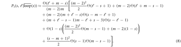
To obtain the full 1-loop protein distribution (equation (4)), we first need to compute the probability for a site to not be part of loop,

If the loop density, ρ, were uniform, we would simply have  , since the 1D cluster has a total length of m + ℓ with a single loop of length ℓ. This uniform condition would only apply if we randomly choose ℓsites to be part of the loop and ignore the requirement that all these loop sites need to be neighboring. In a real cluster, however, we expect the loop density ρloop(s) to be higher in the bulk of the 1D cluster than close to the parS site or the edges, because fewer loops can be formed near the parS site or near the boundaries of the 1D cluster, at which a protein must be bound by construction. In particular, we expect the loop density,
  , which measures the number of ways a site at s can be part of a loop. This results in the normalized probability

In the normalization of this expression we distinguish the cases where the loop is either smaller or larger than the number of proteins in the cluster. With equations (8) and (10), we have all the elements to calculate the 1-loop protein binding profile P1(s, ℓ) from equation (4).
We investigated the binding profiles P1(s, ℓ) predicted by this model for a selected set of parameters, as shown in figure 3. We only show s > 0 because of the symmetry of the binding profile. It is instructive to contrast these profiles with the triangular profile (black curve) for a cluster with no loops. As expected, the addition of loops widens the profile, allowing the tail of the distribution to extend out to a distance m + ℓ. The widening of the binding profile is accompanied by a faster decay of the profile in the vicinity of parS, which crosses over to a flatter profile at distances s > ℓ due to additional contributions from configurations where the loop lies between the parS site and site s.
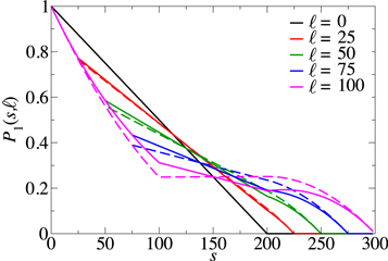
Figure 3. Protein occupation probability, P1(s, ℓ), for a site a genomic distance s (in units of ParB footprint, 16bp) from the parS site for different loop lengths ℓ and a fixed cluster size of m = 200 proteins. All distances are measured in units of the ParB footprint on DNA. Solid curves represent analytic calculations from equations (4), (8), and (10), and dashed curves represent data obtained from exact numerical enumeration for comparison with our analytical approximations. We note that for ℓ = 0, we recover the triangular profile of the S&B model in the strong coupling limit  [31].
[31].
Download figure:
Standard image High-resolution imageInterestingly, for large loop size the profile can even become non-monotonic with a slight increase near the far edges of the domain. These features of the profile reflect the reduced loop density near parS and near the far edges of the cluster. Note that the integral under this curve remains constant for varying ℓto conserve the number of particles in the cluster. To verify the validity of the analytical approximations leading to P1(s, ℓ), we used exact enumeration as a benchmark. Overall, the numerics (dashed lines) and the analytics (solid lines) are in good agreement for the 1-loop case, as shown in figure 3. In the next section, we employ the approximate analytical expressions obtained above, to efficiently calculate the full binding profile averaged over all configurations.
4. Protein binding profiles and statistics of the LC model
Above we defined the LC model and calculated the binding profile of proteins around a parS site for a cluster with 1 loop with fixed length. Real protein-DNA clusters, however, are expected to fluctuate with new loops forming and disappearing continuously. To capture such fluctuations, we will use the expressions for the binding profile of a static cluster with fixed loop length together with a statistical mechanics description of the LC model to obtain average binding profiles for dynamic clusters, including an ensemble average over both the number of loops and the loop lengths.
To obtain a full binding profile averaged over all realizations, it is useful to investigate the statistics of loops that extend from the protein-DNA cluster and how these statistics are determined by the underlying microscopic parameters of the model. We start by considering the number of loops that extend from the cluster. Using the partition function in equation (3), it is possible to calculate the basic features of the LC model. For instance, the moments of the distribution of the number of loops are given by

From this, we find the the average loop number is given by

where  is the renormalized loop activation energy introduced in equation (3). The average loop number
  is depicted in figure 4(a), demonstrating the exponential dependence on the spreading energy JS. In figure 4(b), we plot
  as a function of the total number of proteins m in the protein-DNA cluster. Indeed, we observe the expected linear dependence of the average loop number
  on m over a broad range of parameters. These results illustrate how the average number of loops is determined by the competition between the effective renormalized loop activation energy,
  (including the cost in loop closure entropy), and the gain in the positional entropy of mixing (see appendix B).
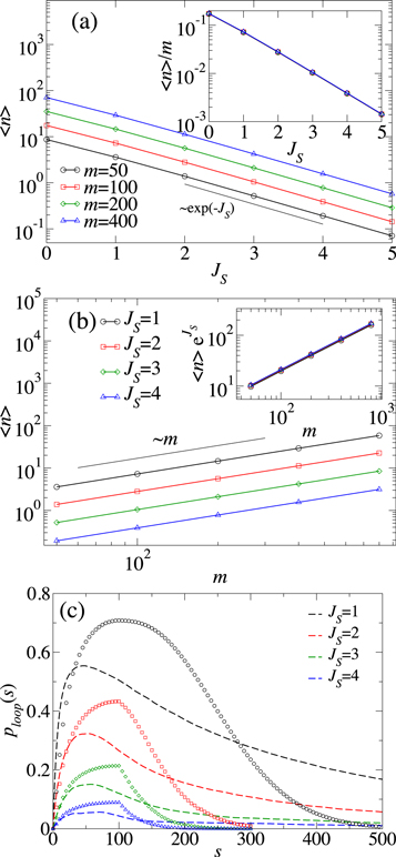
Figure 4. (a) Average number of loops,  , as a function of the spreading coupling strength JS obtained from equation (12). The different curves correspond to protein number m = 50 (black), m = 100 (red), m = 200 (green), and m = 400 (blue), with loop-size cutoff ℓ0 = 10. We observe an exponential decrease
  in accordance with equation (12). Inset: same data replotted with the expected dependence of the average loop number on m scaled out. (b) Average number of loops
  as a function of m for JS = 1, 2, 3, and 4. The behavior is linear as expected from equation (12). The prefactor that determines the vertical shift between the different curves scales with
  , as demonstrated in the inset of panel (b). (c) Average loop probability as a function of the genomic coordinate with m = 200 and L = 4000 for protein-DNA clusters with fluctuating loop number and loop lengths. Different curves correspond to different spreading couplings JS = 1, 2, 3, and 4. The analytic approximation (symbols) using equation (15) for the loop density, averaged over different loop configurations with the appropriate Boltzmann factor as in equation (14), is compared to MC simulations (dashed curves) of the LC model (see appendix A).
Download figure:
Standard image High-resolution imageThe linear dependence on m in equation (12) reflects that loops are assumed to be able to form anywhere in the cluster in the LC model. However, one would naively expect that loops can only form at the surface of a 3D cluster, resulting in a dependence  for a compact, spherical cluster. However, Monte Carlo simulations of the full S&B model have revealed that the protein-DNA clusters are not compact [31], but rather have a surface that scales almost linearly in m, close to the behavior of the simplified LC model presented here. The non-compact nature of the protein-DNA cluster is perhaps not surprising because each protein can form only one bridging bond.
A closely related statistic is the average accumulated loop length  . From the LC partition function, we notice that the loop length is completely decoupled from the coupling constant JS and depends only on the upper cutoff ℓmax. Therefore, the cumulated average loop length becomes

where the factor in front of  represents the average length per loop. This prefactor induces a small algebraic dependence on ℓmax, in contrast to
  which depends only on the lower cutoff ℓ0.
The loop statistics of protein-DNA clusters are not easily accessible in experiments. Instead, the most relevant results for which this model can provide insight come from ChIP-Seq experiments. These experiments yield data for the enrichment of bound ParB as a function of genomic position on the DNA, providing a measure of the average protein binding profile of ParB on DNA [26, 27]. In the LC model, the ParB density profile along DNA can be calculated from

where ZLC is given in equation (3). Here,  represents the multiloop ParB binding profile with n loops of length {ℓi} = {ℓ1, …, ℓn}. For simplicity, we approximate this multiloop profile by the analytical 1-loop conditional probability, P1(
 ), with the loop length equal to the accumulated loop length, i.e.
  , weighted by the loop probability
  . In the expression for the loop probability, ρ(s, m, ℓi, ℓ) is defined as the contribution to the loop density of a loop of length ℓi in a cluster of m proteins with a total accumulated loop length ℓ, and we neglected correlations between contributions from different loops. Furthermore, we approximate ρ(s, m, ℓi, ℓ) by using a generalization of the 1-loop expression in equation (10),

In the analysis above, we aimed to capture the effects of multiple loops in a simple way by assuming statistical independence of the loops, and by using the analytical 1-loop expressions to approximate the impact of loop formation on the loop density and the ParB binding profile of the protein-DNA complex. To test the validity of these approximations, we performed MC simulations of the complete LC model. We find that the numerically obtained average loop probability is in reasonable agreement with our approximate expression for the multiloop density, as shown in figure 4(c). Thus, despite the simplicity of our approach, the analytical model provided here captures the essential features of looping in protein-DNA clusters.
The protein binding profile PLC(s) around a parS site is calculated by averaging the static binding profile for different total loop numbers and loop lengths using the Boltzmann factor (see equation (3)) from the LC model as the appropriate weighting factor. The resulting expression in equation (14) for the protein binding profile of a protein-DNA cluster is the central result of this paper. We use this expression to compute binding profiles for the full LC model, which are shown in figure 5 as a function of the distance s to parS for m = 100, 200, and 400. By construction, the site s = 0 corresponding to parS is always occupied, and thus P(s = 0) = 1 for all values of the spreading energy JS. This feature of the LC model captures the assumed strong affinity of ParB for a parS binding site. For JS = 4, the binding profile converges to a triangular profile, implying a very tight cluster of proteins on the DNA with almost no loops. The triangular profile in this case results from all the distinct configurations in which this tight cluster can bind to DNA such that one of the proteins in the cluster is bound to parS, and therefore the probability drops linearly to 0 at s ≈ m. The same triangular binding profile was observed for the S&B model in the strong coupling limit  [31]. Interestingly, as JS becomes weaker, we observe a faster decrease of the binding profile near parS together with a broadening of the tail of the distribution for distances far from parS. This behavior results from the increase in the number of loops that extrude from the ParB-DNA cluster with decreasing spreading bond strength JS. The insertion of loops in the cluster allows binding of ParB to occur at larger distances from parS. Thus, the genomic range of the ParB binding profiles is set by
  , where the average cumulated loop length
  is controlled by JS (see equation (13)) and m. These results illustrate how the full average binding profile is controlled by the spreading bond strength JS: the weaker JS, the looser the protein-DNA cluster becomes, which results in a much wider binding profile of proteins around parS. In the limit
  , the LC model quantitatively reduces to the statistics of non-interacting loops, as shown in the inset of figure 5. In this case, the binding profiles exhibit asymptotic behavior
  for large s, as in the stochastic binding model [27]. Interestingly, we observe a weaker scaling PLC(s) with s at intermediate genomic distances, which we attribute to the reduced loop density near parS (see figure 4(c)).
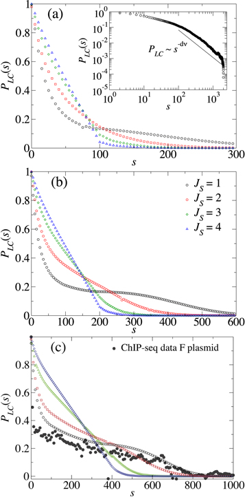
Figure 5. Binding profiles of ParB from equation (14) plotted versus the genomic distance s to parS for (a) m = 100, (b) 200, and (c) 400. In equation (14), the loop size integrals were calculated with a lower cutoff ℓ0 = 10 and an upper cutoff of 10 ℓ0; summations were truncated at n = 15. The dark gray circles in panel (c) show experimental ChIP-Seq ParB enrichment data from the F-plasmid of E. coli extracted from [27]. The inset in panel (a) shows the binding profile of ParB versus genomic distance s from parS for JS = 1, ν = 0.588 (self-avoiding polymer). The results in this inset were obtained by Monte Carlo simulations of the LC model (see A.1 for details). The data plotted on a log-log scale show the power law decay PLC ∼ s−dν expected in the limit of low JS, where the LC model becomes conceptually similar to the stochastic binding model.
Download figure:
Standard image High-resolution imageTo investigate how the functional shape of the binding profile is determined by the total number of proteins in the cluster, we plot the binding probability versus the scaled variable s/m for m = 100, 200, and 400, as shown in figure 6. For fixed JS, the data approximately collapse onto a single curve as a function of the scaled distance s/m. This implies that the functional shape of the ParB binding profile is largely determined by the spreading bond strength JS, while the number of proteins in the cluster determines the width of the profile.
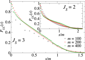
Figure 6. Scaling function of the ParB binding profile for different total protein numbers m (same data as in figure 5). The data for the different total protein number m are plotted versus the dimensionless genomic distance s/m from parS (main graph: JS = 3, inset: JS = 2).
Download figure:
Standard image High-resolution image5. Discussion
The LC model introduced here allows us to access the average binding profile of proteins making up a large 3D protein-DNA complex. In our model, the formation of a coherent cluster of ParB proteins is ensured by a combination of spreading and bridging bonds between DNA bound proteins, which together can drive a condensation transition in which all ParB proteins form a large protein-DNA complex localized around a parS site [31]. We do not assume, however, that this protein-DNA cluster is compact. Indeed, loops of protein-free DNA may extend from the cluster, which strongly influences the average spatial configuration of proteins along the DNA. In the LC model, the formation of loops in the protein-DNA cluster is controlled by the strength of spreading bonds, i.e. the bond between proteins bound to nearest neighbor sites on the DNA. Specifically, for every protein-free loop of DNA that extends from the cluster, a single spreading bond between two proteins within the cluster must be broken. Thus, if the spreading interaction energy, JS, is sufficiently small, thermal fluctuations will enable the transient formation and breaking of spreading bonds, thereby allowing multiple loops of DNA to emanate from the protein cluster (see figure 1).
Conceptually, the spreading bond interaction determines how ‘loose’ the protein-DNA cluster is, which directly impacts the ParB binding profiles. When JS is large, loop formation is unlikely, resulting in a compact protein-DNA cluster with a corresponding triangular protein binding profile centered around parS [31]. At intermediate JS, the protein-DNA cluster becomes looser with the formation of loops, resulting in a binding profiles that are more strongly peaked around parS but with far-reaching tails. Importantly, the LC model enables us to establish a link between the spreading and bridging model and the stochastic binding model [27]. The first used a microscopic approach based on the types of interactions between proteins on the DNA polymer, while the second employed a more macroscopic approach based on the polymer configurations around a dense sphere of proteins. In the limit JS → 0, the LC model is consistent with the stochastic binding model with a profile of the form [27] given by  (inset figure 5(a)). Thus, the LC model offers a description for a broad parameter regime, connecting two limits investigated in preceding studies [27, 31]. Therefore, our work also resolves the apparent contradiction between these previous models.
The LC model, which we introduce to calculate the binding profile of ParB-like proteins on the DNA, is a simple theoretical framework similar to the Poland–Scheraga model for DNA melting [39, 40]. An important difference in the LC model with respect to the homogeneous Poland–Scheraga model, is that translational symmetry is broken due to the presence of a parS site at which a protein is bound with a high affinity. Thus, the protein-DNA cluster can adopt a wide range of configurations as long as one of the proteins is bound to the parS site. As a result, loops are effectively excluded in the vicinity of parS. The central new result of this work is a simple way of computing the protein binding profiles around such a parS site in terms of molecular interactions parameters. We show that the binding profiles predicted by this model are sensitive to both the expression level of proteins and the spreading interaction strength, which directly controls the formation of loops in the protein-DNA cluster. The LC model predicts a profile in good quantitative agreement with binding profiles measured with ChIP-Seq on the F-plasmid of E. coli, as shown in figure 5(c). Importantly, from this analysis we extract the spreading interaction strength JS ≈ 1kBT and the number of proteins in the cluster m ≈ 400. The value of m is consistent with estimates based on quantitative Western blots [27]. The quantity JS is a more challenging quantify to estimate, but gel-shift or similar assays could be used on short DNA oligomers to estimate this spreading bond strength.
Our results also have implications for experiments that employ fluorescent labeling of DNA loci by exogenous ParBs [28, 29]. Indeed, our model can be used to investigate how the protein interaction strengths determine the 3D structure and mobility of the ParB-DNA cluster, as well as the tendency of multiple ParB foci to adhere to each other. This model thus provides an insightful quantitative tool that could be employed to analyze and interpret ChIP-Seq and fluorescence data of ParB-like proteins on chromosomes and plasmids.
Acknowledgments
This project was supported by the German Excellence Initiative via the program NanoSystems Initiative Munich (NIM) (CPB), the Deutsche Forschungsgemeinschaft (DFG) Grant TRR174 (CPB), and the National Science Foundation Grant PHY-1305525 (NSW). The authors acknowledge financial support from the Agence Nationale de la Recherche (IBM project ANR-14-CE09-0025-01) and from the CNRS Défi Inphyniti (Projet Structurant 2015-2016). This work is also part of the program ‘Investissements d’Avenir’ ANR-10-LABX-0020 and Labex NUMEV (AAP 2013-2-005, 2015-2-055, 2016-1-024). We also thank J-Y Bouet for helpful comments on the manuscript.
Appendix A.: Monte Carlo simulations and numerical integration procedures
A.1. Monte Carlo procedure
Using the partition function, we can formulate an effective 1D Hamiltonian for the LC model, which explicitly accounts for the spreading bonds and loop entropy:

This effective Hamiltonian is useful to perform Monte Carlo simulations of the model as a benchmark for the approximations performed in the analytical approach (see figure 7). The proteins are modeled as particles that bind/unbind onto sites of a one-dimensional lattice with free boundary conditions. The lattice size L = 4000 is chosen to prevent finite size effect for the range of proteins considered. Note that, in these MC simulations, the total size of the loops is limited to L − m.
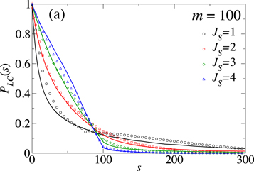
Figure 7. The binding profile obtained with the analytic approach (14) (symbols) are compared to MC simulations (solid lines) for m = 100, ℓ0 = 10 and JS = 1, 2, 3 and 4.
Download figure:
Standard image High-resolution imageThe simulations are performed with the standard Metropolis rules:
- 1.Propose a move of a particle randomly chosen to a random empty site of the lattice (conserved order parameter). A MC iteration step consists of m attempts of move.
- 2.Calculate the difference of energy
 between final and initial configurations.
 - 3.If, the move is accepted with probability 1, otherwise it is accepted with probability .


The system is set initially with all particles in a single cluster ( ), and then thermalized to the actual JS of the simulations ranging from 1 to 4 (see figure 7). The sampling starts after thermalization of the system (40 000 MC iterations). A sampling of the systems configuration is performed every 100 MC iterations. All MC averages have been performed over 107 configurations, ν = 0.588, L = 4000 and ℓ0 = 10. The numerical results of this Monte Carlo simulation are in good agreement with our approximate analytic results, as shown in figure 7.
A.2. Numerical integration
To evaluate the binding profile PLC(s), we proceeded as follows. We carried out the evaluation of the simplified expression in equation (14) using numerical summation and integration. We truncated the summation at n = 15, instead of going up to m − 1, based on the corresponding average number of loops of figure 5. Finally, we introduced an upper cutoff for the loop-length, ℓmax = 100, instead of going up to infinity. We confirmed that shape of the binding profiles does not change significantly for higher values of ℓmax = 100.
The numerical evaluation of the multidimensional integrals in equation (14) have been performed with an accuracy and precision of respectively 2 and 3 effective digits in the final results. We have carried out convergence tests of the curve shapes in order to assess our parameter choice and rule out numerical instabilities. All computations have been performed by routines written in the Wolfram Language and executed by the Mathematica software suite (version 10 and 11).
Appendix B.: Formal connection between the LC model and a Lattice Gas with renormalized coupling
For m, n ≫ 1 (thermodynamic limit), we can formulate a saddle point approximation to evaluate the partition function and  , by approximating the entropic (factorial) term in Z (equation (11)) using the standard entropy of mixing for placing n loops on m − 1 possible sites. This approach gives physical insight into how the loop entropy contributes to a renormalized protein–protein interaction and how the competition between this renormalized interaction and the entropy of mixing controls
  . Taking the thermodynamic limit leads to a partition function:

where ρℓ = n/(m − 1) is the concentration of loops (0 ≤ ρℓ ≤ 1) and

an effective free energy where  is a loop activation energy renormalized by the cost in loop entropy with
  . In the limit
  , the approximate partition function
  becomes exact and can be evaluated exactly in the saddle point approximation by minimizing Feff. The solution, ρSP, to the saddle point equation, dFeff(ρℓ)/dρℓ = 0, is

The entropic contribution to Feff (second term) vanishes at ρℓ = 0 and 1, and reaches a minimum at ρℓ = 1/2, which is the exact result for ρSP at vanishing renormalized loop activation energy  because the entropy of mixing is then maximized. For
  decreases from 1/2 to vanish in the limit
  as
as  . In this limit only the no and one loop states contribute and the asymptotic behavior can be simply obtained by a series expansion of the partition sum and the corresponding expression for
  . The saddle point result leads to

which turns out to be the exact result, thanks to compensating errors, for  for finite m (which can be obtained by differentiating the exact Z with respect to JS, see equation (12)). For example, for ℓ0 = 10, d = 3, and ν = 0.588, α0 = 4.437 and ln(α0) = 1.49, which is not negligible if
  .
.
Footnotes
- 5
Although this reasoning is not strictly true for self-avoiding polymers, it does hold if we adopt the usual approximation used in the Poland–Scheraga model for DNA melting that self-avoidance acts only within individual loops.