ABSTRACT
Supermassive black holes are believed to be ubiquitous at the centers of galaxies. Measuring their masses is extremely challenging yet essential for understanding their role in the formation and evolution of cosmic structure. We present a direct measurement of the mass of a black hole in an active galactic nucleus (Arp 151) based on the motion of the gas responsible for the broad emission lines. By analyzing and modeling spectroscopic and photometric time series, we find that the gas is well described by a disk or torus with an average radius of 3.99 ± 1.25 light days and an opening angle of 68.9+21.4 − 17.2 deg, viewed at an inclination angle of 67.8 ± 7.8 deg (that is, closer to face-on than edge-on). The black hole mass is inferred to be 106.51 ± 0.28 M☉. The method is fully general and can be used to determine the masses of black holes at arbitrary distances, enabling studies of their evolution over cosmic time.
1. INTRODUCTION
In the past decade, it has become clear that supermassive black holes are a fundamental ingredient of the universe (Ferrarese & Ford 2005). Accretion onto their deep gravitational potential is responsible not only for some of the most powerful sources of light (Lynden-Bell 1969), but also appears to be a key ingredient for the formation and evolution of galaxies (Granato et al. 2004; Croton et al. 2006). Energy released by the accretion mechanism is believed to play a role in regulating the heating and cooling of interstellar gas, and therefore the formation of stars. The “smoking gun” of this connection between galaxies and black holes is the tight correlation between the mass of black holes and the stellar velocity dispersion σ* of their host galaxies, observed at small redshifts (Ferrarese & Merritt 2000; Gebhardt et al. 2000). This correlation represents the endpoint of the so-called coevolution of galaxies and black holes, though it is still unclear how galaxies and black holes coevolve across cosmic time. Both galaxies and black holes are believed to grow by mergers and accretion from initial perturbations of the density field in the early universe; however, it is not yet known whether galaxies and black holes grow in lockstep, or one of the two forms first and subsequently acts as a seed for the other.
The main challenge in mapping the coevolution across cosmic time is determining black hole masses. Traditional methods rely on spatially resolved kinematics of stars and gas within the gravitational sphere of influence of the black hole. Therefore, they are only applicable with current technology in the very local universe (Ferrarese & Ford 2005). Alternative methods are needed to measure black hole masses out to distances of several billion light years—look-back times corresponding to a sizable fraction of the present-day age of the universe (Komatsu et al. 2011).
Reverberation mapping is the most promising method for measuring the masses of black holes powering active galactic nuclei (AGNs) at cosmologically interesting distances (Blandford & McKee 1982; Peterson 1993; Peterson et al. 2004). The technique is made possible by the temporal variations in the intrinsic brightness of the central continuum source and by the subsequent response of line-emitting gas well within the gravitational sphere of influence of the black hole, known as the broad-line region (BLR). By measuring the time delay (or lag) τ between the variations of the continuum and the variations of the broad emission lines, the physical size of the BLR can be determined. In addition, the typical orbital velocity of the broad-line gas can be measured from the width of the broad lines themselves, σl. Combining this velocity measurement with the radius yields an estimate of the mass of the central black hole, MBH = fσ2lcτ/G (Peterson et al. 2004), where f is the so-called virial coefficient, c is the speed of light, and G is the gravitational constant.
Despite the simplicity of the reverberation mapping idea, its practical implementation is beset with numerous difficulties (e.g., Krolik 2001). First, in its standard implementation, the formula connecting black hole mass to spectral line width and the time lag includes a virial coefficient that depends on the unknown geometry of the orbiting BLR gas (Onken et al. 2004; Woo et al. 2010; Greene et al. 2010; Decarli et al. 2011). Second, the adopted approach is usually indirect: the data are used to measure properties of the transfer function describing the distribution of lags, or simply the mean lag. To constrain properties of the BLR gas distribution itself, another layer of modeling is necessary to reveal which possible BLR geometries are consistent with the inferred transfer function (Bentz et al. 2010).
We overcome these difficulties by applying a new framework to modeling high-quality spectrophotometric monitoring data of the Type 1 active nucleus of Arp 151. The combination of dynamical models with high-quality data allows us to characterize the structure of the BLR and achieve a direct determination of the mass of a supermassive black hole using reverberation mapping. Our measurement is independent of any external information on the virial coefficient.
2. DATA AND MODELING FRAMEWORK
The data were collected as part of the Lick AGN Monitoring Project (LAMP) campaign (Bentz et al. 2009; Walsh et al. 2009). They consist of 84 epochs of photometric monitoring and 43 epochs of spectroscopic monitoring of the region containing the Hβ emission line (Bentz et al. 2009; Walsh et al. 2009). The continuum and line flux temporal series are shown in Figure 1. The Hβ spectral time series is illustrated in the left panel of Figure 2 (wavelength on the abscissa, epoch on the ordinate; the epochs are approximately one day apart, but not exactly, due to gaps and scheduling issues).
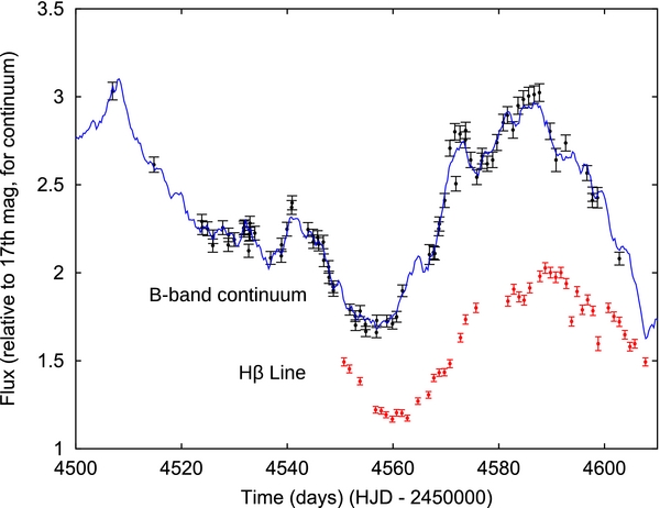
Figure 1. Continuum flux time series from LAMP, and the corresponding Hβ flux time series. The curve drawn through the continuum data shows a realization of an interpolation of the continuum data using Gaussian processes.
Download figure:
Standard image High-resolution image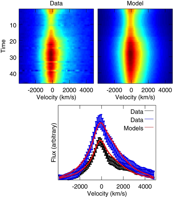
Figure 2. Top left: measured spectrum of the broad Hβ emission line as a function of epoch; these are the data used for our inference. Top right: model-predicted spectrum as a function of time, using parameter values chosen at random from the posterior distribution. The major features of the data (time variation, line widths) are reproduced by our model. Bottom: example of the spectral line shape at two times, along with model fits.
Download figure:
Standard image High-resolution imageIn order to infer the BLR geometry and the black hole mass, we take a Bayesian Inference approach to the problem (Sivia & Skilling 2006). We construct a model characterized by a finite number of parameters describing the black hole mass, the spatial density profile of the BLR and its kinematic structure, and the intrinsic continuum light curve, denoting these parameters collectively by Φ. We define broad prior probability distributions for Φ and then define the probability distribution for the data, conditional on knowledge of all of these properties p(D|Φ). Given specific data, the prior distribution gets updated to the posterior distribution which describes knowledge of the parameters after taking into account the data, using Bayes’ rule  . In practice, we quantify our results by generating randomly sampled models from the posterior distribution using a Nested Sampling method (Brewer et al. 2010).
The physical model consists of a large number (1000) of BLR clouds that are in orbit in the Keplerian potential of the central black hole. The spatial distribution of the clouds is generated using a flexible model that is capable of representing generic geometries including thin disks and tori as well as complete spheres and shells. By applying spatially varying illumination to the clouds, we can also describe non-axisymmetric geometries. The cloud emission is assumed to respond linearly to continuum variations. Therefore, the observed spectrum at a given time is the result of the continuum emission at earlier times, with time lags corresponding to the optical path from the central continuum to the cloud to the observer. The configuration of a model that well represents the data is illustrated in Figure 3.
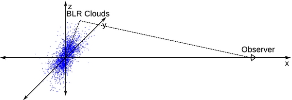
Figure 3. Distribution of extra path lengths the light must travel from the central engine to a BLR cloud and then to the observer is the cause of the delayed response of the emission-line flux, and the variations in line shape. The distribution of BLR gas in this diagram corresponds to a probable configuration inferred from the Arp 151 data.
Download figure:
Standard image High-resolution imageFitting of models to the data requires knowledge of the continuum flux at all times, not just the measured times. To solve this problem, our method uses Gaussian processes to interpolate and extrapolate the continuum light curve taking errors into account. A typical intrinsic light curve generated by this process is shown in Figure 1. Thus, our results include uncertainty caused by the fact that we have noisy measurements of the continuum flux at a finite number of times. Our modeling of the continuum light curve is similar to that independently developed by Zu et al. (2010) and used outside of reverberation mapping in studies of quasar variability (e.g., Kozłowski et al. 2010; Kelly et al. 2009; MacLeod et al. 2010). Additional information on the method in general is given by Pancoast et al. (2011, hereafter P11).
3. THE DYNAMICAL MODEL
We do not aim to infer the position and velocity of each cloud from the data, but rather to use the clouds to map out a spatial and dynamical model described by a small number of hyperparameters. This approach is equivalent to that followed by P11, except that we are using Monte Carlo samples of clouds to represent the distribution of BLR gas as opposed to computing the density on a spatial grid. To generate a three-dimensional distribution of BLR clouds, we start by generating an axisymmetric distribution in the x–y plane, and then apply rotations to “puff up” the model into a three-dimensional configuration. Finally, we weight the clouds by a non-axisymmetric illumination function to model non-axisymmetric distributions of gas.
The distance of a cloud from the black hole is prescribed according to  , where F ∈ [0, 1] and
  is drawn from a gamma distribution with mean μ and standard deviation βμ. With this prescription, μ is the overall mean radius, F is the fraction of the mean radius that is due to the hard lower limit, and β ∈ [0, 1] describes the shape of the distribution; β ≈ 1 is an exponential distribution, and β ≈ 0 is a narrow normal distribution. The polar coordinate ϕ of a cloud is chosen uniformly from [0, 2π].
For the inference, the priors on these parameters are as follows. We use a uniform prior for β, a scale invariant ∝1/x prior for μ (between generous limits), and a uniform prior for black hole mass given μ, such that the predicted line widths are on the order of those in the data, reducing the volume of parameter space that needs to be explored.
We then assign cloud velocities in a probabilistic manner (note that we can assign multiple velocities to each cloud in order to improve sampling of the phase space in a computationally efficient way; throughout this Letter, we adopt 100 velocities for each of the 1000 clouds). As in P11, we assume that the only force acting on the BLR clouds is gravity from the central black hole.
The total energy of a cloud at a distance r from the black hole, moving with angular momentum L, is given by

which has the minimum possible value

If we knew the position, energy, and angular momentum of a cloud, we could solve for the radial velocity,

We choose the negative (inbound) solution with probability q and the outbound with probability 1 − q, a free parameter. For solutions to exist, the angular momentum must satisfy

Circular orbits are obtained if we set the energy and angular momentum to


To get elliptical orbits, instead of assigning E and L the exact circular values above, we assign them at random from the following probability distributions:

where 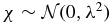 , and
, and

These probability distributions are centered around the values for circular velocities, but the parameter λ describes the dispersion, or how noncircular typical orbits will be. The circular orbit formulae are reproduced when λ → 0. The probability distributions for E and L given three different values for λ are shown in Figure 4, along with the corresponding line shapes. For the inference, we use a uniform prior on λ between 0 and 1.
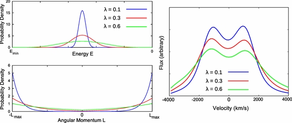
Figure 4. Probability distributions for energy and angular momentum that generate elliptical orbits for the clouds. The effects on the predicted line shape are illustrated for an edge-on disk for three different values of the “noncircularity parameter” λ.
Download figure:
Standard image High-resolution imageThe main advantage of our implementation of this method with respect to that of P11 is that we can generate relatively broad distributions of E and L with a smaller number of parameters. The drawback is that this model is technically nonstationary (in the case of noncircular orbits) and would change if it were allowed to evolve in a dynamically self-consistent way. Our model can be thought of as describing the time-invariant illuminated part of the full phase-space distribution, even though the underlying particles are actually flowing through the region. We checked that this simplifying assumption does not bias our inference on the black hole mass by analysis of the data with the code developed by P11. The results are consistent with the ones presented here.
We then rotate the models (positions and velocities of the clouds) by an appropriate distribution of angles to generate an axisymmetric distribution of angular momentum vectors. The first rotation is about the y-axis by a small random angle; the typical size of these angles determines the opening angle of the disk or torus. We then rotate around the z-axis by random angles to restore the axisymmetry of the model. Finally, we rotate again about the y-axis by the inclination angle to model the inclination of the system with respect to the line of sight. For the inference, we use uniform priors on the opening angle and the inclination angle.
To obtain non-axisymmetric models, in order to reproduce the line asymmetry, we weight each cloud by a simple spatially varying illumination function. In spherical polar coordinates, this function is

where ![$\kappa \in [-\frac{1}{2}, \frac{1}{2}]$](https://content.cld.iop.org/journals/2041-8205/733/2/L33/revision1/apjl391448ieqn5.gif) is a free parameter with a uniform prior. Positive κ illuminates the front portion of the BLR, while negative κ illuminates the back. We also implemented, as a secondary check, a model with a different (linear in x) functional form for the illumination, but this model did not reproduce the data as well, although the final black hole mass estimate was similar. In predicting the observed spectra, we included the narrow-line component as a constant which does not respond to the continuum variations.
is a free parameter with a uniform prior. Positive κ illuminates the front portion of the BLR, while negative κ illuminates the back. We also implemented, as a secondary check, a model with a different (linear in x) functional form for the illumination, but this model did not reproduce the data as well, although the final black hole mass estimate was similar. In predicting the observed spectra, we included the narrow-line component as a constant which does not respond to the continuum variations.
4. RESULTS AND CONCLUSIONS
Our results are presented in Figure 5. We find that the geometry of the BLR is well described by a thick disk or torus (opening angle 68.9+21.4 − 17.2 deg), viewed at an inclination 67.8 ± 7.8 deg (where 0° = edge-on and 90° = face-on), as depicted in Figure 3. This geometry is consistent with the hypothesis that Type 1 AGNs are viewed close to face-on, if the dusty torus is coplanar with the BLR. The mean radius μ of the disk is 3.99 ± 1.25 light days, and the radial profile is inferred to be close to exponential (β = 0.86+0.10 − 0.19). We note that four light days corresponds to <10−5 arcsec at the distance of Arp 151 (redshift 0.021), an angular size more than a thousand times smaller than what can be resolved even with the Hubble Space Telescope. The orbits of the BLR clouds are found to depart significantly from circular, and there is no strong evidence favoring either inflow or outflow (see Figure 5).
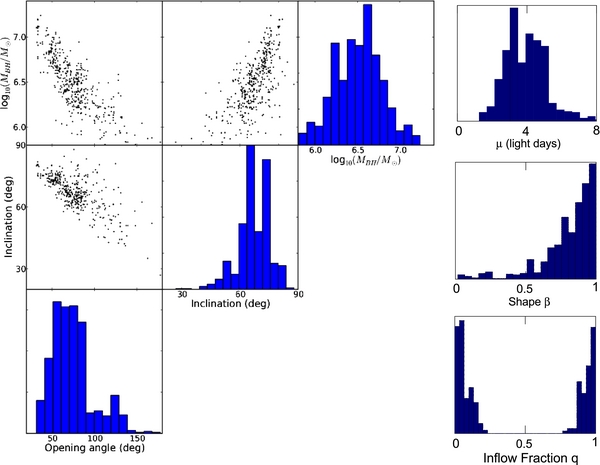
Figure 5. Joint and marginal posterior distributions for the parameters of the BLR geometry and kinematics. The strongest correlation is between the inclination angle and the opening angle of the disk. Both of these parameters are also strongly correlated with the black hole mass.
Download figure:
Standard image High-resolution imageWe note that the posterior distribution does not rule out radial profiles that peak close to r = 0, which is unphysical due to the high ionizing flux from the accretion disk (Korista & Goad 2004). However, conditioning on the peak of the radial profile being at the high end of the posterior does not significantly change any inferences except for the inflow fraction q: inflow becomes favored by a ratio of 70:30 if we assume the density peaks at r > 1 light day. Thus, there is weak evidence for inflow, as found by Bentz et al. (2010). If inflow is present, then the front of the disk must be more visible than the back (i.e., κ > 0), either because of obscuring material or nonuniform illumination effects.
By marginalizing over all of the model parameters, we derive the posterior probability distribution function for the central black hole mass. The median and 68% credible interval are 106.51 ± 0.28 M☉. This is lower than, but overlaps with, the value of 106.85 ± 0.07 M☉ obtained by Bentz et al. (2009) assuming log10f = 0.74 based on requiring active and inactive galaxies to obey the same correlation between MBH and host-galaxy stellar velocity dispersion σ* (Onken et al. 2004), and neglecting uncertainty in f. Recent measurements suggest that the intrinsic uncertainty in f from this method is at least 0.4 dex (Woo et al. 2010; Greene et al. 2010). Reversing the traditional argument, our measurement implies that log10f = 0.40 ± 0.28, a low value, for this particular system. Modeling a larger sample of systems and comparing the results of traditional methods with our direct approach would allow us to test the assumption that active galaxies obey the same MBH−σ* relation as inactive galaxies (Davies et al. 2006; Hicks & Malkan 2008; Onken et al. 2007).
To summarize, our measurement has three key advantages with respect to traditional methods. First, it is direct, independent of any assumption regarding the correlations between supermassive black holes and their host galaxies, thus allowing us to test this assumption. Second, it provides a more precise measurement (smaller formal uncertainties) than traditional methods. Finally, the outputs of the inference procedure are physical properties of the BLR, rather than a transfer function, bypassing the need for an additional modeling step.
We conclude by listing some of the limitations of this work and the prospects for future improvements. In our dynamical model we neglect radiation-pressure support and the dynamical influence of the accretion disk itself, as is commonly the case in traditional reverberation mapping analysis. We also neglect the optical depth of the BLR clouds themselves (Bottorff et al. 1997). If the motion of the BLR clouds were partially supported by radiation pressure, then we would be underestimating the mass of the central black hole. This is currently a topic of debate (Marconi et al. 2008; Netzer & Marziani 2010), and external information needs to be used to break the degeneracy between black hole mass and pressure support. Once external information is available, it can easily be taken into account in interpreting our results.
On a more detailed level, our model for the spatial profile of the BLR is significantly oversimplified with respect to the real physical picture. Thus, we cannot reproduce all features of the observed line profiles (Figure 2). Neglecting this systematic uncertainty would lead us to underestimate the uncertainty in the parameter values. In this study, we addressed this issue by inflating the observed error bars (see Figure 2) until the model reproduced just the macroscopic features of the emission lines. In other words, we do not expect to be able to model all features of the lines, to within the given noise level. Inflating the measurement error bars on the data protects our results from some (but not all) systematic errors, particularly those that would result in fluctuations in the line profiles smaller than the domain of the data. See Brewer et al. (2011) for a discussion of this issue.
For these reasons, our uncertainty in the black hole mass is significantly larger than what the method can in principle deliver for data of comparable quality in the absence of modeling errors, ∼0.05 dex (P11). In addition, our model neglects collisional effects as well as anisotropic winds, which could change somewhat the dynamics and geometry of the BLR, but should not affect the inference on black hole mass as long as gravity is the dominant force.
Thus, modeling uncertainties dominate over measurement uncertainties, driving the total uncertainty in black hole mass. Therefore, the next step toward improving the overall precision of the measurement is to develop more flexible and physically realistic models. Such models will also allow us to explore in more detail the kinematics of the BLR.
B.J.B., A.P., and T.T. acknowledge support by the NSF through CAREER award NSF-0642621, and by the Packard Foundation through a Packard Fellowship. In addition, A.P. is funded by the NSF Graduate Research Fellowship Program. The LAMP project was also supported by NSF grants AST-0548198 (UC Irvine) and AST-0507450 (UC Riverside). A.V.F. is grateful for the financial support of NSF grant AST-0908886 and the TABASGO Foundation. J.H.W. acknowledges support by the Basic Science Research Program through the National Research Foundation of Korea funded by the Ministry of Education, Science and Technology (2010-0021558). B.J.B. thanks Matt Auger for assistance with plotting, and Greg Dobler and Sebastian Hoenig for useful suggestions. We thank W. P. McCray for useful comments that improved the clarity of the manuscript, and the anonymous referee for suggestions that improved the modeling.