ABSTRACT
We predict the spatial distribution and number of Milky Way dwarf galaxies to be discovered in the Dark Energy Survey (DES) and Large Synoptic Survey Telescope (LSST) surveys, by completeness correcting the observed Sloan Digital Sky Survey dwarf population. We apply most massive in the past, earliest forming, and earliest infall toy models to a set of dark matter-only simulated Milky Way/M31 halo pairs from the Exploring the Local Volume In Simulations project. Inclusive of all toy models and simulations, at 90% confidence we predict a total of 37–114 L ≳ 103 L☉ dwarfs and 131–782 L ≲ 103 L☉ dwarfs within 300 kpc. These numbers of L ≳ 103 L☉ dwarfs are dramatically lower than previous predictions, owing primarily to our use of updated detection limits and the decreasing number of SDSS dwarfs discovered per sky area. For an effective rlimit of 25.8 mag, we predict 3–13 L ≳ 103 L☉ and 9–99 L ≲ 103 L☉ dwarfs for DES, and 18–53 L ≳ 103 L☉ and 53–307 L ≲ 103 L☉ dwarfs for LSST. We also show that the observed spatial distribution of Milky Way dwarfs in the LSST-era will discriminate between the earliest infall and other simplified models for how dwarf galaxies populate dark matter subhalos.
1. INTRODUCTION
In a universe described by a Λ+cold dark matter cosmology (ΛCDM; Planck Collaboration et al. 2013), the predicted number of dark matter subhalos far exceeds the observed number of dwarf galaxies orbiting Milky-Way-(MW)-like galaxies. In the time since this discrepancy was dubbed “the missing satellites problem” (Kauffmann et al. 1993; Klypin et al. 1999; Moore et al. 1999), more than a dozen previously unseen ultra-faint (L ≲ 50,000 L☉) Local Group dwarfs have been discovered, primarily in Sloan Digital Sky Survey (SDSS; e.g., Willman 2010, and references therein) and PAndAS (e.g., Martin et al. 2013a, 2013b) data. However, it is not yet clear whether the observed number, spatial distribution, and masses of these discoveries are consistent with CDM-based expectations (Weinberg et al. 2013).
A common approach to the cosmological interpretation of the MW's dwarf population is to predict the number (e.g., Tollerud et al. 2008) and spatial distribution (e.g., Willman et al. 2004; Macciò et al. 2010; Yniguez et al. 2014) expected in surveys, such as the Dark Energy Survey (DES; The Dark Energy Survey Collaboration 2005; Rossetto et al. 2011) and the Large Synoptic Survey Telescope (LSST; Ivezic et al. 2008). Such predictions are typically either (1) based on an N-body simulation+semi-analytic galaxy formation model (Macciò et al. 2010; Bovill & Ricotti 2011; Font et al. 2011), or (2) a completeness correction of the known number of MW dwarfs, using a physically motivated spatial distribution (Koposov et al. 2008; Tollerud et al. 2008; Walsh et al. 2009). All past predictions for ultra-faint dwarf galaxies in DES and LSST have been subject to one or more limitations: (1) the use of only one average model or a single simulation to predict the spatial distribution of ultra-faint dwarfs, (2) the use of isolated (rather than paired MW/M31) galaxy simulations, (3) the inclusion of “hyperfaint” (L ≲ 103 L☉) dwarfs such as Segue 1 in the same predictions as more luminous dwarfs, or (4) the application of rigid magnitude limits for DES and LSST.
In this Letter, we take steps to overcome these limitations using the Exploring the Local Volume In Simulations (ELVIS; Garrison-Kimmel et al. 2014) suite of N-body simulations, plus physically motivated toy models for populating subhalos with galaxies. We predict a spatial distribution of MW dwarf galaxies and correct the MW dwarf galaxy count for completeness. In Section 2 we summarize our toy models. In Section 3 we discuss the predicted spatial distributions of dwarfs, and in Section 4 we present our predicted numbers. We summarize our expectations for DES and LSST in Section 5.
2. DWARF GALAXY TOY MODELS
Owing to observational bias, the underlying spatial distribution of the MW's dwarf galaxy population is unknown. To statistically correct the observed number of MW dwarfs, we use spatial distributions of dark matter subhalos in the ELVIS simulations. ELVIS includes a dozen dark-matter-only, cosmological zoom-in simulations of MW and Andromeda pairs (see Garrison-Kimmel et al. 2014 for details). We consider the galaxy in each simulated pair with the lower virial mass to be the MW analog. The particle mass in the high-resolution regions of the fiducial simulations is mp = 1.9 × 10⁵ M☉. The simulation suite includes isolated simulations of each of the MW and Andromeda analogs at the same resolution, with three simulated at a higher-mass resolution of mp = 2.35 × 10⁴M☉. The fiducial subhalo catalogs are complete to Vmax = 8 km s−1 and Vpeak = 12 km s−1.
To generate statistical descriptions for the spatial distribution of MW dwarfs, we implement three physically motivated toy models for which subhalos of the ELVIS MW analogs host dwarf galaxies—most massive in the past, earliest forming, and earliest infall. The first two models have been implemented in a number of past studies (e.g., Bullock et al. 2000; Strigari et al. 2007; Kravtsov 2010). For all models we exclude any subhalos with Vpeak > 25 km s−1, as their deeper potential wells are likely to host the more luminous “classical” dwarfs.
- 1.Massive in the past (Vpeak > 12 km s−1). Subhalos with deeper potential wells are more likely to retain and cool the gas fuel necessary for star formation. Vpeak is the historical peak of a subhalo's circular velocity curve and provides a measure of potential well depth. We tested threshold values for Vpeak of 12 km s−1 and higher, and found an average of ∼100 subhalos per MW-massed primary for Vpeak > 15 km s−1 and ∼200 for Vpeak > 12 km s−1. Although the typical number of subhalos in the higher threshold model is a better match to the predicted number of ultra-faint dwarfs, the spatial distribution of the higher threshold model is similar. We therefore implement the Vpeak > 12 km s-1 cut to improve statistics.
- 2.Formed before reionization (z > 8 and Npart ⩾ 32). Another hypothesis is that the ultra-faint dwarf galaxies are “fossil” that produced the bulk of their stars prior to reionization (Bovill & Ricotti 2011). This hypothesis is supported by photometric and spectroscopic studies of ultra-faint dwarfs, which show that these galaxies formed their stars within ∼1 Gyr of each other at early times (Sand et al. 2010; Brown et al. 2012; Kirby et al. 2013; Frebel et al. 2014). We follow the Bovill & Ricotti (2011) definition of reionization fossils as galaxies residing in halos with Vpeak < 20 km s−1, and which had a resolved progenitor in the ELVIS paired simulations at z = 8. These thresholds result in ∼170 subhalos per MW analog.
- 3.Earliest infall (zpeak ⩾ 3, i.e., tinfall ≳ 11.5 Gyr ago, and Vmax > 8 km s−1). An alternative model to explain the truncated star formation histories of ultra-faint dwarfs is that early infall into the MW's halo resulted in massive gas stripping (e.g., Weisz et al. 2014). Many of the MW's ultra-faint dwarfs show spatial or kinematic hints of tidal disturbance (Muñoz et al. 2010; Willman et al. 2011; Sand et al. 2012), which might be expected among dwarfs that have been orbiting within the MW's potential for the longest time, and with (on average) relatively smaller orbital pericenters. Because subhalos typically reach Vpeak just before infall onto a larger halo (Behroozi et al. 2014), we adopt the redshift of peak circular velocity as our estimate of the infall time. To avoid overestimating the Poisson contribution to our uncertainties, for this model we exclude the four ELVIS pairs with resulting subhalo counts less than the number of ≳ 103 L☉ dwarfs expected from an area-only correction (∼34; Zeus and Hera, Sonny and Cher, Hall and Oates, Thelma and Louise). This model yields ∼56 subhalos per MW analog.
2.1. Numerical Testing
Figure 1 compares the cumulative radial profile of each toy model applied to: the 12 MW analogs from the paired fiducial simulations, the corresponding 12 isolated fiducial simulations, the 3 high-resolution isolated simulations, and the 3 corresponding fiducial isolated simulations.
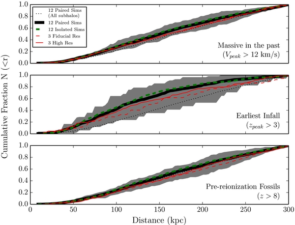
Figure 1. Comparison of the cumulative radial distribution of subhalos for the three toy models: massive in the past (top panel), earliest infall (middle panel), pre-reionization fossils (bottom panel). Shown are the mean profiles for the 12 paired (solid black), 12 isolated (dashed green), and 3 isolated fiducial (dashed red line) and high-resolution (solid red line) simulations. The mean of the 12 paired fiducial resolution simulations is shown for comparison (dotted line). The gray region shows the simulation-to-simulation scatter from the 12 paired simulations.
Download figure:
Standard image High-resolution imageThese comparisons demonstrate that the radial distributions of subhalos in the paired and isolated simulations are indistinguishable, and the high-resolution and fiducial-resolution simulations are statistically the same when comparing the same three simulated halos. The range of radial profiles from the 12 paired MW analogs are also shown, with the earliest infall model showing a large halo-to-halo variation. We will further discuss these radial distributions in Section 3.
A mild caveat for the ELVIS-based radial distributions is that baryonic physics can decrease the survivability of subhalos with small orbital pericenters. For example, tidal shocking of satellites by the MW's disk can accelerate mass loss (D'Onghia et al. 2010). Supernova feedback may yield cored density profiles in the most luminous dwarf satellites, making them more vulnerable to destruction (Zolotov et al. 2012; Brooks et al. 2013). The former issue is more relevant to the ultra-faint dwarfs than the latter (Governato et al. 2012). However, both effects should drive the true surviving subhalo population to be less concentrated than the ELVIS toy models. Thus our predictions may be lower limits to the expected satellites counts in future surveys.
3. PREDICTED SPATIAL DISTRIBUTION OF DWARFS
A complete census of dwarfs out to the MW's virial radius should provide the statistics needed to use the observed radial distribution of dwarfs to discriminate between some toy models for how dwarfs populate subhalos (e.g., Gao et al. 2004; Willman et al. 2004; Rocha et al. 2012; Wang et al. 2013). Figures 1 and 2 show that the earliest infall subhalos are significantly more centrally concentrated than the most massive and earliest forming subhalos, which have very similar spatial distributions to that of all subhalos resolved in ELVIS.4
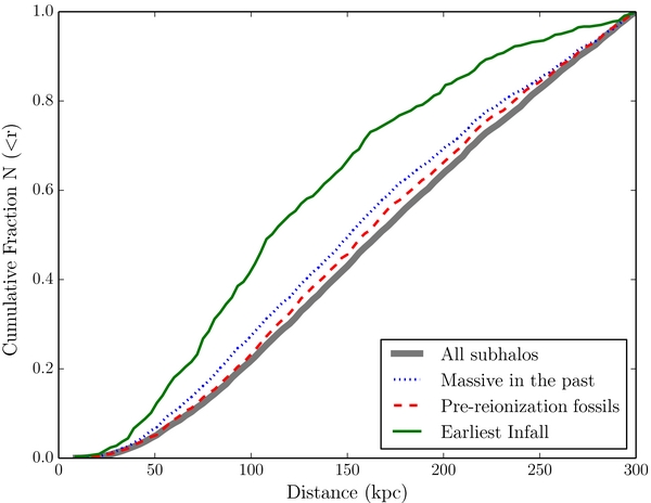
Figure 2. Comparison of the mean cumulative radial distributions of subhalos for the 3 toy models applied to the MW analog in the 12 ELVIS paired simulations.
Download figure:
Standard image High-resolution imageThe lack of MW dwarf discoveries between the SDSS Data Release 6 (DR6, 9583 deg2, 12 dwarfs) and Data Release 8 (DR8; 14555 deg2, 2 additional dwarfs) has recently re-invigorated the discussion of the population's azimuthal anisotropy. Inspired by this observational result, we explored ΛCDM expectations by generating 100 mock survey pointings for each of five survey areas (1000–14, 500 deg2) in both the paired ELVIS MW analogs and a set of azimuthally uniform subhalo distributions (“Poisson” expectations). The survey-to-survey variation in subhalo counts (for the median of all simulations) is marginally consistent with Poisson expectations on survey scales larger than ∼10,000 deg2. On smaller survey scales, however, Poisson fluctuations are a lower limit to the expected survey-to-survey variations. Most ELVIS simulations (∼9 of the 12) show survey-to-survey variations of up to twice those of Poisson expectations, although usually only ∼25%–50% more variation, underscoring the importance of accounting for azimuthal variations when making predictions (see Section 4). We also note the importance of considering the bias against the detection of dwarfs within 25°of the MW's disk (Walsh et al. 2009). For example, the lack of dwarfs discovered in SDSS DR8 is consistent with Poisson expectations (and therefore with ΛCDM, to zeroth order) if one only considers the 2900 deg2 of new imaging area at |b| > 25° between SDSS DR6 and DR8.
To look specifically for evidence of a systematic alignment of subhalos along the MW–M31 axis, we generated smoothed spatial maps of the resolved subhalo distributions (stacked, medians, and individual), rotated to place the simulated M31 analog at the same Galactic coordinates as M31. Although the stacked map showed a suggestive trend, we did not find a statistically significant global trend in the alignment of the subhalo distribution relative to M31. Examining the individual maps showed that only three paired simulations displayed an overdensity of subhalos in the direction of the M31 analog (Burr and Hamilton, Scylla and Charybdis, and Kek and Kauket).
4. PREDICTED NUMBERS OF DWARFS IN DES AND LSST
We make our predictions using a method similar to Tollerud et al. (2008). Our approach has two steps: (1) completeness correcting the observed MW dwarfs to the total number of expected within 300 kpc (approximately the MW virial radius) within a randomly placed mock-SDSS footprint, then (2) scaling that result to a randomly placed mock DES (5000 deg2) or LSST (20,000 deg2) survey with some magnitude limit. Our choice of 300 kpc as the outer radial limit is consistent with the mean virial radius (as defined in the ELVIS simulations) of the MW analogs. For each toy model and each fiducial survey magnitude limit, we simulate 100 mock-SDSS + DES/LSST survey pointings in each MW analog in the 12 paired ELVIS simulations. These mock survey pointings do not mimic the relative sky pointings of the actual surveys.
We adopt 12,000 deg2 for the mock-SDSS survey area. This corresponds to the area of DR8 with uniform detection limits, specifically excluding |b| < 25° (Walsh et al. 2009), and it includes all 14 dwarfs discovered in SDSS. Our correction only includes these 14 dwarfs, because we assume that dwarfs similar to those previously known would have already been detected at |b| > 25° (Willman 2010). Our dwarf sample includes 10 L ≳ 103 L☉ dwarfs (Hercules, Boötes I, Leo IV and V, Pisces II, Canes Venatici I and II, UMa I and II, Coma Berenices) and four “hyperfaint” L ≲ 103 L☉ dwarfs (Boötes II, Willman 1, and Segue 1 and 2). The boundary at L ∼ 103 L☉ loosely corresponds to those objects that can only be discovered by main sequence turnoff stars and fainter (too few red giant branch stars).
For each dwarf, the corrected number within the SDSS footprint is 1/(fraction of toy model subhalos within the maximum detection distance). We calculate each dwarf's maximum detection distance, dmax, SDSS, using the 90% SDSS detection efficiency function given by Walsh et al. (2009). This fraction is normalized to unity for dmax, SDSS = 300 kpc. Only CVn I has dmax, SDSS > 300 kpc, resulting in no completeness correction. The values of dmax, SDSS for CVn II, Psc II, and Leo V are smaller than their observed distances, so we adopt dobserved as their dmax, SDSS's and perform an additional efficiency correction based on an estimated integrated detection efficiency within dobserved from Walsh et al. (2009, = 1.0, 0.5, and 0.85 respectively). Objects like the other 11 SDSS dwarfs were detected with 100% efficiency with the Walsh et al. (2009) algorithm, unlike the Koposov et al. (2008) algorithm—the primary source of the difference between our and the Tollerud et al. (2008) results.
To scale the corrected numbers within the SDSS footprint to the expected numbers in each mock DES or LSST survey, we account for both survey area and point-source detection limit. Rather than scaling directly by relative survey area, we scale by the ratio of the number of subhalos within dmax, survey of a mock survey area to the number within dmax, survey of a mock SDSS. This captures the azimuthal anisotropy in the ELVIS simulations, allowing us to directly incorporate the effect into our uncertainties. We naively assume that completeness distances scale like the flux depth of each survey (dmax, survey = dmax, SDSS × 10 ), given rlim, SDSS = 22.0 mag. In light of the challenges separating resolved stars from unresolved galaxies at faint apparent magnitudes, we consider 23.3 < rlim, survey < 25.8 for both DES and LSST.
We apply a slightly different method to the hyperfaint dwarfs, because the numbers of subhalos within their dmax, SDSS (≲ 50 kpc) are too small to provide robust mock survey results. In some toy models, several MW analogs have no subhalos within the dmax of Seg 1 (∼30 kpc). We therefore used azimuthally averaged radial distributions to predict an average number for each simulation and used the mock survey approach to estimate the 10/90 percent confidence intervals. We ignored any random mock survey pointing without a Segue 1-like subhalo. The resulting predictions do not properly capture halo-to-halo and spatial anisotropy uncertainties, but they provide reasonable limits on the uncertainty in the predicted numbers.
The top and bottom panels of Figure 3 show the predicted numbers of L ≳ 103 L☉ and L ≲ 103 L☉ dwarfs as a function of r-magnitude depth. We adopted the median and 10/90 percent confidence intervals from the 1200 mock surveys as our estimated number and uncertainty. The uncertainty on each number reflects both halo-to-halo and survey-to-survey (radial and azimuthal) variations.
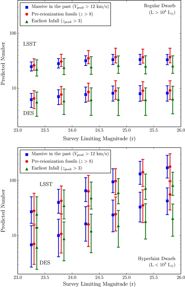
Figure 3. Predicted number of ultra-faint dwarfs for each of the three toy models as a function of survey r-band limiting magnitude for LSST and DES. The results for the brighter and fainter subsets of the ultra-faints are shown in the top and bottom panels, respectively. The error bars show the 10%/90% confidence intervals as described in Section 4.
Download figure:
Standard image High-resolution image5. DISCUSSION
Using our approach of correcting the known population of SDSS dwarfs, we find that the use of paired versus isolated simulations does not yield systematically different predictions for the MW's dwarf population. Although there is statistically significant super-Poisson azimuthal anisotropy in the toy model subhalo distributions, this anisotropy appears neither extreme nor systematically aligned with M31. We also noted that Poisson statistics alone can explain the seemingly low number of SDSS dwarf discoveries post-SDSS DR6 (see Section 3), when the bias against finding dwarfs at low Galactic latitude is considered.
We predict vastly different numbers of regular (L ≳ 103 L☉) versus hyperfaint (L ≲ 103 L☉) dwarfs (see Tables 1 and 2). Spanning all toy models, at 90% confidence, and assuming rlimit = 25.8 mag: 3–13 regular versus 9–99 hyperfaints should be discovered in DES and 18–53 regular versus 53–307 hyperfaints should be discovered in LSST. Over the entire sky and within 300 kpc, we predict ∼37–114 regular and ∼131–782 hyperfaint dwarfs with 90% confidence (see Table 2). Owing to the severely limited numbers of subhalos within dmax for the hyperfaint dwarfs, those predicted numbers are less robust and should be interpreted lightly in future observational studies. We emphasize that these numbers assume no future bias against discovering dwarfs at low Galactic latitude. Any interpretation of future observational studies must also cautiously account for this bias.
Table 1. Predicted Number of Dwarf Galaxies for LSST and DES
| DES (±10/90) | LSST (±10/90) | |
|---|---|---|
| L > 103 L☉, rlim = 23.8 | ||
| Massive in the past |  |
 |
| Pre-reionization fossils |  |
 |
| Earliest infall |  |
 |
| L < 103 L☉, rlim = 23.8 | ||
| Massive in the past |  |
 |
| Pre-reionization fossils |  |
 |
| Earliest infall |  |
 |
| L > 103 L☉, rlim = 25.8 | ||
| Massive in the past |  |
 |
| Pre-reionization fossils |  |
 |
| Earliest infall |  |
 |
| L < 103 L☉, rlim = 25.8 | ||
| Massive in the past |  |
 |
| Pre-reionization fossils |  |
 |
| Earliest infall |  |
 |
Download table as: ASCIITypeset image
Table 2. Predicted Number of Dwarf Galaxies within d = 300 kpca
| All Sky (±10/90) | |
|---|---|
| L > 103 L☉ | |
| Massive in the past |  |
| Pre-reionization fossils |  |
| Earliest infall |  |
| L < 103 L☉ | |
| Massive in the past |  |
| Pre-reionization fossils |  |
| Earliest infall |  |
Note. aThese numbers do not include objects like the “classical” dwarf galaxies.
Download table as: ASCIITypeset image
The predicted number of L ≳ 103 L☉ dwarfs is strikingly lower than previous predictions (e.g., Tollerud et al. 2008) due to our use of updated detection limits, the decreased rate of SDSS dwarfs discovered per sky area, our toy models, and a 300 kpc distance limit. The lower limit on the predicted number of L ≳ 103 L☉ is similar to a simple area correction, because a mock SDSS can include an overdensity of subhalos and because the radial distribution of the early infall model of some MW analogs is very centrally concentrated. The discovery of only a few dwarfs in DES imaging (for a shallow survey limit of r ∼ 23.8) could be consistent with our lower limits.
The predicted total numbers of dwarfs are not significantly different between the most massive in the past or the pre-reionization models, but the earliest infall model systematically predicts lower total numbers of dwarfs by a factor of ∼2. The discoveries of small numbers of dwarfs in future surveys would provide support for an early infall, or other centrally concentrated, model. However, such hypotheses may be more sensitively tested by the observed radial distribution of dwarfs (e.g., Section 3, Figure 1).
Table 1 summarizes our DES and LSST predictions for two effective survey depths, rlim = 23.8 and 25.8 mag. Both of these are shallower than the expected surveys' 5σ point-source detection limits. The shallower limit is a pessimistic estimate of the effective survey depth possible for studies of low-surface brightness objects if color-based methods to separate stars from unresolved galaxies are not successful, while the deeper limit may be achievable with color-based, probabilistic star–galaxy separation (Fadely et al. 2012).
Within their footprints, and at high Galactic latitudes, DES and LSST (single visit) should easily recover the full population of MW dwarfs similar to those known with L ≳ 103 L☉. Mining point-source catalogs fainter than r ∼ 24 mag will primarily yield the detection of increasing numbers of hyperfaint dwarfs, when only considering the dwarf population within 300 kpc. Given the enormous range of possibilities for the MW's dwarf population, the coming decade will bring another wild ride of discovery through our Galaxy's halo.
B.W. and J.H. were supported by an NSF Faculty Early Career Development (CAREER) award (AST-1151462). This work was also supported in part by National Science Foundation grant No. PHYS-1066293 and the hospitality of the Aspen Center for Physics. We thank the anonymous referee for timely and very helpful comments on the manuscript. We acknowledge Shea Garrison-Kimmel for helpful conversations and for sharing the ELVIS data. We thank Tim Beers for inspiring our use of the term “hyperfaint” dwarf. We also acknowledge useful conversations with Mike Boylan-Kolchin, Andrew Wetzel, Erik Tollerud, and Alis Deason.
Footnotes
- 4
Although the radial distribution of the ELVIS subhalos is more spatially extended than the MW's classical dwarfs, it is consistent with M31's bright dwarf satellites (Yniguez et al. 2014). However, incompleteness limits our knowledge of the observed distribution of MW dwarfs (Willman et al. 2004). We specifically exclude the subhalos which may host classical dwarfs in our analysis (see Section 2), because we are modeling ultra-faint dwarfs which may have a different underlying spatial distribution. We note that more centrally concentrated spatial distributions would result in lower numbers of predicted dwarfs relative to more spatially extended profiles.