Abstract
We present a method for solving the constraint equations in the Hassan–Rosen bimetric theory to determine the initial data for the gravitational collapse of spherically symmetric dust. The setup leads to equations similar to those for a polytropic fluid in general relativity, here called Lane–Emden-like equations. Using a numerical code which solves the evolution equations in the standard 3 + 1 form, we also obtain a short-term development of the initial data for these bimetric spherical clouds. The evolution highlights some important features of the bimetric theory such as the interwoven and oscillating null cones representing the essential nonbidiagonality in the dynamics of the two metrics. The simulations are in the strong-field regime and show that, at least at an early stage, if the bimetric initial data are close to those for general relativity, the bimetric evolution stays close to the evolution in general relativity as well, and with no instabilities, albeit with small oscillations in the metric fields. In addition, we determine initial data and first evolution for vacuum bimetric spherically symmetric nonstationary solutions, providing generic counterexamples to a statement analog to Jebsen–Birkhoff theorem in bimetric relativity.
Original content from this work may be used under the terms of the Creative Commons Attribution 4.0 licence. Any further distribution of this work must maintain attribution to the author(s) and the title of the work, journal citation and DOI.
1. Introduction
In comparison to general relativity (GR), the phenomenology of the Hassan–Rosen (HR) bimetric relativity [1–4] is at an early stage, and the full extent of its physical features is still unknown. At present, bimetric theory is compatible with Solar System and cosmological data [5]. In GR, numerical relativity plays an important role in theoretical astrophysics to clarify structure formation and growth, or formation processes of black holes. Only by means of numerical simulation and experiments, it is possible to get a theoretical understanding of such phenomena occurring in nature [6–10]. In particular, numerical relativity is essential in analyzing strong-field gravitational systems to interpret gravitational wave detections [11]. Similar remarks also hold for the HR theory. In order to perform bimetric numerical simulations (and discriminate bimetric from GR predictions), many questions need to be addressed; for example [12]:
- (a)Which initial data solve the bimetric constraints for gravitational collapse?
- (b)Which formalism to use for stable bimetric numerical evolution?
- (c)What are appropriate gauge conditions?
- (d)What algorithms provide numerical stability?
- (e)What are suitable boundary conditions for numerical grids?
- (f)What is a good method for finding the apparent horizon?
To obtain reliable numerical results, all of these issues have to be resolved.
This work belongs to a series of papers in which we aim to investigate the above issues. Earlier papers in this series establish the bimetric equations in the standard 3 + 1 form [13], and calculate the ratio of lapse functions for the case of spherical symmetry [14]. In the current paper, we present a method for solving the bimetric constraints to determine the initial data for the gravitational collapse of dust in the HR theory. Using a numerical code based on the equations of motion in the standard 3 + 1 form, we then obtain a short term development of the initial data. Obtaining a long term bimetric development is the subject of ongoing work. In order to achieve a more stable numerical evolution, [15] establishes the covariant Baumgarte–Shapiro–Shibata–Nakamura (cBSSN) formalism [16–20] for bimetric relativity. A class of gauge conditions specific to the HR theory are treated in [21].
This paper is structured as follows. The rest of this section summarizes the results by examples; it also reviews the basic equations. Section 2 poses and solves the bimetric constraint equations. Section 3 highlights the properties of the evolution of the initial data. The paper ends with a brief discussion and outlook.
1.1. Summary of results
We consider the case where the two metric sectors are spherically symmetric with common SO(3) Killing vector fields [22]. In GR, with a pressureless dust perfect fluid and spherical symmetry, the Lemaître–Tolman–Bondi spacetime is an analytical solution [23–25]. In bimetric theory, there are no analog solutions, as shown in [26].
In GR, the kinematical and dynamical parts of a metric field can be separated using the 3 + 1 formalism [27, 28]. The same procedure can be applied to bimetric theory using a suitable parametrization based on the geometric mean metric [13]. In this context, the general form of the two metrics in spherical polar coordinates reads,


where α and  denote the lapse functions, β and
  are the radial components of the shift vectors, and
  denote the nontrivial components of the spatial vielbeins. In addition, we also evolve the nonzero components of the extrinsic curvature,

The radial components of the shift vectors are conveniently redefined in terms of the mean shift q and the separation parameter p [13],

In this parametrization, the lapses α,  , and the mean shift q do not appear in the constraint equations. All the variables in (1.1a)–(1.3) are functions of (t, r).
We start from the development of existing GR initial data for g, hereinafter called the reference GR solution. At this stage we decouple f; the bimetric theory is reduced to two copies of GR where we only consider the evolution in the g-sector containing the collapsing matter (letting f evolve in parallel, for instance, a Minkowski solution). The bimetric interaction will be engaged in a second stage, treating the bimetric collapse after knowing the behavior of the reference GR solution2.
As a reference GR solution, we consider a spherical dust cloud with arbitrary density profile at t = 0. The initial data can be constructed using the time symmetric initial condition where the extrinsic curvature is vanishing, assuming the conformally flat spatial metric. The initial values for the density with a Gaussian profile and the corresponding metric field A are shown in figure 1. The development of this initial data forms a black hole [30].
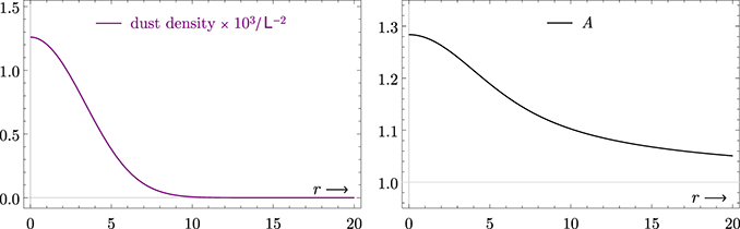
Figure 1. Initial data for the reference GR solution where the density profile of dust is Gaussian at t = 0. The radial coordinate is in units of the black hole mass (formed after the collapse).
Download figure:
Standard image High-resolution imageAfter constructing the reference GR solution, we engage the two sectors through the bimetric interaction and solve the bimetric constraint equations for the metric fields, keeping the same matter profile coupled to g. This results in a system of coupled differential equations whose solution depends on the parameters of the HR theory. The construction of the bimetric initial data is the topic of section 2. Typical initial values for the metric fields A and  which are far from the GR limit are shown in figure 2. These fields carry physical content for the observers in the respective metric sector; they roughly correspond to gravitational potentials in the Newtonian limit.
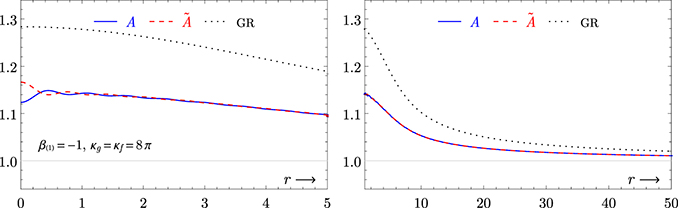
Figure 2. An example of bimetric initial data obtained by deforming the reference GR solution in figure 1. The bimetric fields A and  are interwoven and oscillate along the radial coordinate.
Download figure:
Standard image High-resolution imageFinally, as described in section 3, we numerically evolve the initial data. The simulations are not long enough to shed light on the end point of gravitational collapse. Nevertheless, the bimetric collapse of the dust cloud stays very close to the reference GR solution, if the initial data is close to the GR initial data, as illustrated in figure 3. More details about the gravitational collapse in the GR limit are given in section 3.3 (see also figures 5 and 18).
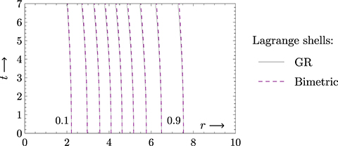
Figure 3. Lagrange shells for the reference GR and the bimetric initial data which are close to GR (the shells are worldlines of Lagrangian matter tracers labeled by the fixed interior rest-mass fraction). The collapse is in the strong-field regime, where almost all of the dust is initially inside r ≈ 8. In GR, the apparent horizon of the formed black hole is at r ≈ 3 after t ≈ 40 (figure 5). The bimetric solution follows GR, showing no instabilities during the initial phase (see section 3.3).
Download figure:
Standard image High-resolution imageTo highlight the bimetric features in the physical content, we employ causal diagrams that display metric configurations according to the method given in [31], an overview of which is given in appendix
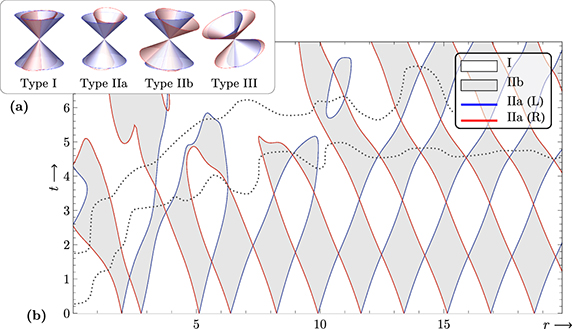
Figure 4. Causal diagram for the evolution of bimetric initial data. These causal types are referring to alignments of the nullcones. Geometrically, they are related how many null directions are shared [3]. The white regions are type I (bidiagonal), the shaded type IIb, and the edges type IIa. Type III does not appear in spherical symmetry because of the dimensional reduction. The dotted lines are isohypses (surface levels) of the l2-norm of the scalar constraint violations (the upper line is at 10−2, the lower at 10−3, with no violations at t = 0; see equation (3.1)). The plot displays the oscillations of the metric fields in space and time.
Download figure:
Standard image High-resolution image1.2. Basic equations
The action of the Hassan–Rosen bimetric theory reads, [33–35],

The metrics g and f are specifically coupled through the ghost-free bimetric potential V(S),

Here,  denotes the principal square root of the (1, 1) tensor field gμρfρν, and en(S) are the elementary symmetric polynomials (the principal scalar invariants of S). The potential is parametrized by dimensionless real constants β(n) with an overall length scale ℓ−2 in the geometrized units c = G = 1. The particular form of the potential is dictated by the necessary condition for the absence of ghosts [36], where the dynamics of each metric is given by a separate Einstein–Hilbert term in the action [1]. The principal branch of the square root ensures an unambiguous definition of the theory [3].
The resulting bimetric field equations are (here stated in the operator form),


where Gg and Gf are the Einstein tensors of the two metrics, κg and κf are Einstein’s gravitational constants, Tg and Tf are the stress–energy tensors of the matter fields each minimally coupled to a different metric sector, and Vg and Vf are the contributions of the bimetric potential (1.5), also called the bimetric stress–energy tensors. The functions Yn(S) in (1.6) encapsulates the variation of the bimetric potential with respect to the metrics,

Note that Y4 ≡ 0 truncates the sums in (1.6) accordingly.
The bimetric stress–energy tensors satisfy the following identities [37, 38],


where ∇μ and  are the covariant derivatives compatible with g and f, respectively. Assuming general covariance of the matter action, the matter conservation laws hold, ∇μTgμν = 0 and
  , and the field equation (1.6) imply the bimetric conservation law,

The two equations in (1.9) are not independent according to the differential identity (1.8b).
The 3 + 1 decomposition. The structure of the bimetric field equations is equivalent to having two copies of GR with the additional stress–energy contributions Vg and Vf coupled through (1.8a); hence, their 3 + 1 split is straightforward, provided that one knows the projections of Vg and Vf [13]. The 3 + 1 decomposition of (1.6) results in two sets of the evolution and constraint equations formally analog to those in GR [6–10].
The constraint equations do not depend on the lapse functions and one shift vector because of the particular form of the potential (1.5). The projection of the bimetric conservation law (1.9) gives one additional constraint [13], equivalent to the additional constraint obtained from the Hamiltonian analysis [4] (the so-called secondary constraint). Moreover, as shown in [4, 39], the preservation of this additional constraint relates the two lapses through a ratio, calculated for the case of spherical symmetry in [14].
Since our focus is not on the evolution equations, their standard 3 + 1 form is given in appendix
2. Initial data
We let matter (if any) be coupled to only one of the metric sectors, here g. The initial values for evolution are subject to certain constraints. In spherical symmetry, the dynamical variables are (A, B, K1, K2) and  . Also, the separation parameter p defines the relative shift between the two metrics (characterizing the relative ‘off-diagonality’ of the metrics). The two lapse functions α,
  , and the mean shift q are kinematical variables and do not appear in the constraint equations. Hence, we need to specify the following metric functions of r at t = 0: A, B, K1, K2,
  ,
,  ,
,  ,
,  , and p. These functions are constrained by five equations, which leaves a lot of freedom in choosing their initial values. In the rest of this section, we state the constraint equations, solve for a reference GR solution, and construct the related bimetric initial data.
2.1. Constraint equations
To write down the constraint equations, we need the 3 + 1 decomposition of the stress–energy tensors. Let  , and
, and  denote the normal, tangential and spatial projections of the total stress–energy tensors V + T in the respective sector. These projections sum up the contribution coming from the bimetric potential, denoted by the upper label ‘b’, and the matter contribution, denoted by the upper label ‘m’; for example, ρ = ρb + ρm.
2.1.1. Bimetric sources
The nonzero components of the projections of Vg are [13],



where J1 ≔ Jrr, J2 ≔ Jθθ = Jϕϕ, J = J1 + 2J2.
Similarly for Vf we have,



where  ,
,  , and
, and 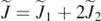 . To simplify equations, we have defined
  and,
and,

The function  encapsulates the β(k)-parameters that do not appear elsewhere. The tangential components satisfy the following identity coming from (1.8a),

2.1.2. Matter sources
We assume that matter is present only in the g-sector and let T ≔ Tg. In particular, we consider a perfect fluid with the stress–energy tensor [7, 40],

where ρ0 is the rest-mass density, h is the specific enthalpy, is the specific energy, P is the pressure, and uμ is the four-velocity of the fluid. The general relativistic hydrodynamic equations consist of the conservation law for Tμν, the conservation law of the baryon number, and the equation of state for the fluid, respectively given by,

Following the 3 + 1 ‘Valencia’ formulation [40, 41], we rewrite (2.6) in the first order flux—conservative form. In spherical coordinates, the resulting equations are expressed in terms of the following conserved variables (here densitizied),

where  is defined in (2.4),
  is the radial component of the Eulerian three-velocity of the fluid, and w is the corresponding Lorentz factor,

The flux—conservative evolution equations for  are relegated to the ancillary file.
For a pressureless fluid (dust), we have P = 0, = 0, h = 1, and the conversion from the conserved to the primitive variables reads,

Finally, the calculation in [40] yields the components of the matter stress–energy tensor,



2.1.3. Bimetric constraints
The scalar and vector constraint equations are obtained as the normal and tangential projections of the bimetric field equation (1.6) on the initial hypersurface. The scalar (or Hamiltonian) constraint equations are,


The vector (or momentum) constraint equations are,


When compared to the full set of constraint equations in four dimensions [13], the angular components of the momentum constraints become trivial. The last two equations can be combined using the identity (2.4),

The separation parameter p can be determined either from (2.11c) or (2.11d).
The bimetric scalar and vector constraints (2.11) are the same as in GR with the addition of the bimetric sources. What is specific to the HR theory is the additional constraint obtained from the projection of the bimetric conservation law,

This constraint eliminates the ghost degrees of freedom. It is obtained using the 3 + 1 projection of the bimetric conservation law, with a general form given in [13] (which is compatible with [4]). Requiring that it stays preserved in time (i.e., ∂tCbim = 0), yields the ratio of lapses [14].
As an example of the bimetric initial data with no matter sources, consider the initial values p = 0,  ,
,  , and
, and  where
where  . These satisfy (2.11)–(2.13) and yield the bi-Minkowski solution.
2.2. Reference GR solution
As mentioned in the introduction, we start from a reference GR solution with decoupled bimetric sectors; we set β(n) = 0 and let the two sectors independently evolve in parallel. This implies  , hence (2.13) identically vanishes at all times. The f-sector is set up to develop the Minkowski solution from the initial data
  ,
,  , and
, and  .
.
The initial data for g are constructed using the time symmetric initial condition,

also assuming a conformally flat spatial metric at t = 0 with the conformal factor ψ(r),

At this point all the bimetric constraints except (2.11a) are satisfied. Hence, ψ and  must satisfy,

where  and Δ denotes the spherical Laplacian. Consider the initial density,

Here, c0 > 0 is a free parameter and erf(z) is the integral of the Gaussian distribution. This density is the same as in [30] for κg = 8π. The solution to (2.16) becomes,

An example of the initial data for  is shown in figure 5; the evolution of these data is treated in section 3, with the results shown in the right panel of figure 5.
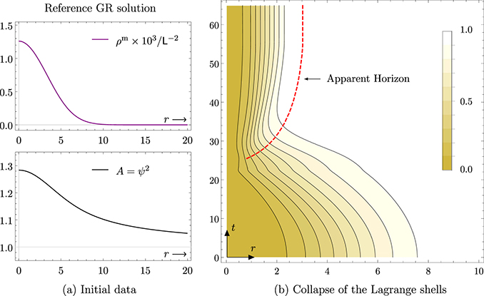
Figure 5. (a) The initial data of the reference GR solution. (b) The development of the initial data forms a black hole. The dashed line shows the apparent horizon. The shells are worldlines of Lagrangian matter tracers labeled by the fixed interior rest-mass fraction (here plotted in the 0.1 or 10% increments).
Download figure:
Standard image High-resolution image2.3. Bimetric spherical cloud
We now engage the bimetric interaction, keeping the same initial density of dust as in the reference GR solution. We again use the time symmetric initial condition with the conformally flat spatial metrics in each sectors,


We set p = 0 but allow for arbitrary β(n)-parameters. The metric configuration is therefore of type I at the initial hypersurface with simultaneously diagonal g and f.
At the moment of time symmetry where  ,
,  , and p = 0, the constraint equations (2.11c), (2.11d), and (2.13) are automatically satisfied. Thus, we only have to consider the scalar constraints (2.11a) and (2.11b); these form a system of Lane–Emden-like equations,


In astrophysics [42], the Lane–Emden equation represents a self-gravitating spherically symmetric fluid with the polytropic equation of state P ∝ ρ1+1/n; in that context, ρ ∝ ϑn satisfies the Lane–Emden equation Δϑ + ϑn = 0. Now, interpreting the conformal factors as gravitational potentials in the Newtonian limit, the metric fields obey deformed equations of states (where the polytropic index becomes definite for a specific β(k)-model in vacuum,  ). In other words, engaging the second metric in an existing GR solution introduces a fluid with nontrivial features in both sectors; this gives the name ‘bimetric spherical cloud’ (referred to as ‘pure’ when
  ). The departure from GR is controlled by the overall factors κgℓ−2 and κfℓ−2.
Given  , the system (2.20) should be solved for ψg(r) and ψf(r). We choose asymptotic boundary conditions where
  , ψg → const, and
  at infinity. This imposes a necessary condition
  for the β(n)-parameters; for example, requiring R∞ = 1 implies,

which fixes β(0) and β(4) in terms of the other parameters. Moreover, in spherical symmetry, the metric components must be even functions of r [43]. Therefore, we use the Neumann boundary conditions at r = 0 requiring ∂rψg = 0 and ∂rψf = 0. Note that we may still choose some arbitrary positive values for ψg and ψf at r = 0.
To summarize: beside κg, κf, β(1), β(2), β(3), ℓ−2, and the density  , we are free to choose ψg and ψf at r = 0, and their ratio at r → ∞. Note that the departure from the reference GR solution is a smooth function of the free parameters (as found by inspection). The GR limit of the HR theory is given by κg/κf → 0 [29, 44–46]. The bounadry value problem was solved using a shooting method, (i.e., as the initial value problem starting from r = 0).
Examples of initial data for different parameter values are shown in figure 6. From the plots we observe higher oscillation frequencies for large β(n)-parameters, which is compliant with the properties of the usual Lane–Emden equation [42, 47]. The leading frequencies for the pure bimetric spherical clouds are shown in figure 7.
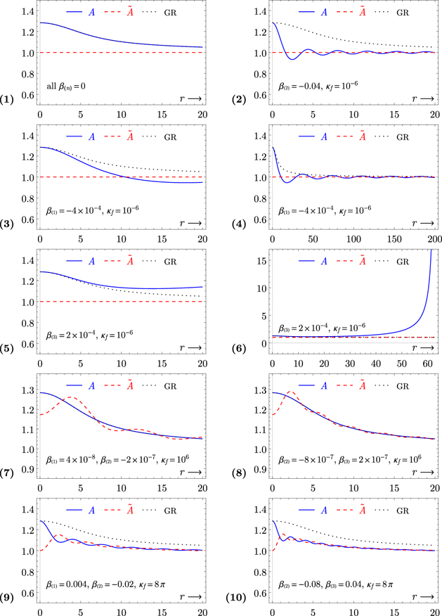
Figure 6. Bimetric spherical cloud examples: (a) decoupled sectors; (b) κf ≪ κg and β(2) = −0.04; (c) and (d) lower frequency modes for β(2) = −4 × 10⁻⁴; (e) and (f) initial data diverging at a finite radius for β(2) = 2 × 10⁻⁴; (g) κf ≫ κg, β(1) = 4 × 10⁻⁸ and β(2) = −2 × 10⁻⁷; (h) κf ≫ κg, β(2) = −8 × 10⁻⁷ and β(1) = 2 × 10⁻⁷; (i) β(1) = 0.004 and β(2) = −0.02 for κf = κg; (j) β(2) = −0.08 and β(1) = 0.04 for κf = κg. All solutions have κg = 8π. The gravitational constants are κf ≪ κg in (a)–(f), κf ≫ κg in (g) and (h), and κg = κf in (i) and (j). The solved initial data may diverge at finite r for some parameters, as in (e). Oscillation frequencies are higher for large β(n)-parameters. Note that  in (a), but
  in (b)–(f). The GR limit is (g) and (h) where κg/κf → 0 and A ≈ AGR.
Download figure:
Standard image High-resolution image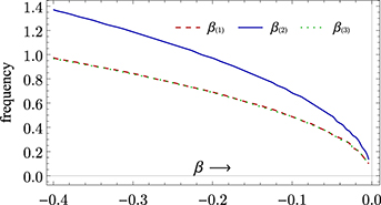
Figure 7. Leading frequencies in the oscillations of A at large radii. The values are extracted from the power spectrum of A, each obtained by solving the initial data for a different β(n)-model.
Download figure:
Standard image High-resolution imageThe preservation of the additional constraint (2.13) relates the two lapses through  where Wg and Wf are functions of dynamical variables [4, 39]. For the case of spherical symmetry, these functions are established in [14]. The relation holds at all times, including t = 0 where it depends on the initial data as shown in figures 8 and 9.
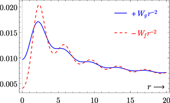
Figure 8. Functions Wg and Wf for the initial data in figure 6 panel 9.
Download figure:
Standard image High-resolution image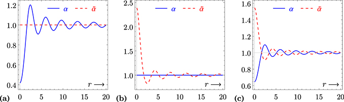
Figure 9. The lapses at t = 0 depending on the gauge (a)  , (b) α = 1, and (c)
  .
.
Download figure:
Standard image High-resolution imageSymmetries in the shapes of Wg and Wf at t = 0 may be used as a guideline to what kind of gauge conditions are preferable for the time slicing, e.g., singling out (c) from figure 9.
3. Dynamical evolution of the initial data
Here we present the solutions obtained from the bimetric initial data. We use a free evolution scheme where the constraint equations are solved at the initial surface and the initial data developed by the bimetric evolution equations. The constraint equations are used as error estimators during the evolution. To evolve the equations, we have written a numerical relativity code package for the bimetric theory, bim-solver [48]. The package is written in C++ and provides a framework that combines the evolution equations generated in mathematica into a functioning bimetric numerical relativity code. The code is OpenMP parallelized [49] and supports MPI [50]. The implementation details for bim-solver will be given elsewhere.
3.1. Formalism and numerical methods
The evolution equations are of the standard 3 + 1 form, given in appendix
The equations are solved using the finite difference approximation in a uniform grid. The implemented spatial difference scheme is centered in space and with arbitrary finite difference order (we have used up to the sixth order). For the time evolution, we employ the method of lines (MoL) using Runge–Kutta (RK) and iterated Crank–Nicholson (ICN) integration. Moreover, Kreiss–Oliger (KO) dissipation has been added for stability [54, 55]. The form of the Kreiss–Oliger operator is taken from [40]. As diagnostics, we monitor the l2-norm of the scalar constraints. The l2-norm of a quantity q is defined by [56],

where the sum goes over all grid points with valid data. As mentioned, the inner boundaries are fixed by mirroring the grid cells around r = 0. The outer boundaries are handled by imposing open boundary conditions. Hence, the ghost cells at r > rmax are updated by extrapolating the interior solution, assuming continuity at the boundary. The extrapolation of the fields is to first order; hence, small unphysical errors are generated in numerical simulations. To delay their propagation, we set the right grid boundary at large radii.
The gauge variables are q, α, and  where the lapses related through
  . The simplest gauge choices are the algebraic: α = 1,
  , or
, or  . The last choice fixes to one the lapse function of the geometric mean metric [13] (other gauges specific to the HR theory are discussed in [21]). Besides using the algebraic gauge conditions, the numerical code also implements the maximal slicing, in this paper used with respect to g.
To detect black hole formation, the code implements an apparent horizon finder in both sectors. In spherical symmetry, a marginally outer trapped surface (MOTS) is given by [6, 57, 58],

The apparent horizon is the outermost MOTS at which (3.2) is satisfied. The solution is obtained using a root-finding algorithm. Alternatively, the function ζ(r) can be plotted, and the apparent horizons determined graphically. Note that MOTS is a geometrical concept of a metric and therefore is also valid in bimetric relativity for each metric separately. The outermost MOTS can be found and plotted for each metric separately; however, their implications on the concept of ‘bimetric event horizon’ are still unknown.
3.2. Simulations
Here we give the numerical details for the simulations and show representative results. We have performed two kinds of simulations:
- (a)Benchmark (diagnostics) simulation for the reference GR initial data,
- (b)Simulations with the engaged bimetric interactions.
For the GR simulation, the grid spacing is Δr = 0.01 with the outer boundary at r = 80. The spatial difference scheme is of the fourth order. The integration employs the method of lines with the third order Runge–Kutta and the Courant–Lax factor (CFL) of Δt/Δr = 0.5. The added Kreiss–Oliger dissipation is of the fourth order with the coefficient 0.03. The lapse is evolved using maximal slicing. The evolution is stable and goes beyond t = 60.
The results of the GR simulation are shown in figure 5, which are compatible with [30]. For comparison, figure 10 shows the solution from figure 5 with an inset that contains datapoints which have been extracted from [30].
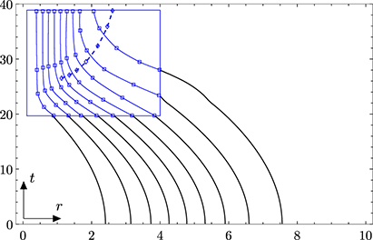
Figure 10. The time variation of the radius of each Lagrange shell for the GR simulation. The inset/overlay shows datapoints extracted from [30] for comparison.
Download figure:
Standard image High-resolution imageAfter the control benchmark, we consider the development of the bimetric initial data constructed in section 2.3. Here we use the grid spacing Δr = 0.04 with the outer boundary pushed to r = 300 and the CFL decreased to 0.25. The code is validated using convergence tests varying Δr by factors of two. Since exact solutions are unknown, we employ a Cauchy-type convergence test using the results obtained at three different resolutions. Denote with f(1), f(2) and f(4) the solutions computed using radial grid spacings Δr, Δr/2 and Δr/4, respectively; then the convergence factor is given by [59],

where n is the order of the sequence of approximations f(1), f(2), f(4). The convergence tests for a solution whose initial data is close to GR are shown in figure 11. The factor remains stable, hence the algorithm converges in the selected range of Δr.
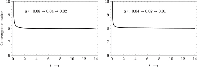
Figure 11. The convergence factor for the sequence of solutions obtained for the scalar constraint at the grid spacing Δr = 0.08 (left panel) and Δr = 0.04 (right panel). The factor 8 indicates the third order of convergence of the scalar constraint to the value zero.
Download figure:
Standard image High-resolution imageNext, we examine the evolution of the metric components to the initial conditions shown in figure 12(a). The metric components have a tendency to become bi-proportional,  and
and  , at least over a short time period as in figure 13. Note that the null cones oscillate over the time; the same figure shows the radial components of the shift vectors at t = 2 and t = 4.5.
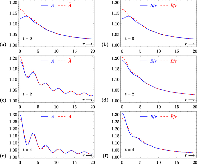
Figure 12. The metric components at t = 0, t = 2, and t = 4. The initial values are for κg = κf = 8π, β(1) = −1, ψg|r=0 = 1.06, ψf|r=0 = 1.08, and R∞ = 1.
Download figure:
Standard image High-resolution image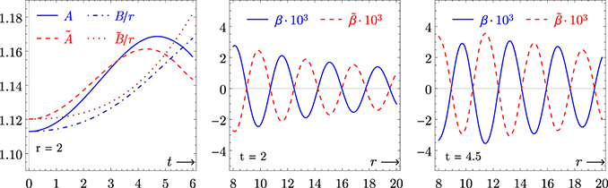
Figure 13. The time variation of A and  at r = 2, and the shift vectors at t = 2 and t = 4.5.
Download figure:
Standard image High-resolution imageThe lapses are evolved using the maximal slicing with respect to g; the proper times of the Eulerian observers for g and f are shown in figure 14. Time is slowed down near the coordinate origin because of the failed regularization. In contrast to the GR simulations that run beyond t > 60, the bimetric evolutions fail within t < 15, mostly because of the violated boundary conditions. The main cause of the instability are irregularities coming from round-off errors when calculating the lapse ratio and the corresponding spatial derivatives near r = 0.
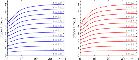
Figure 14. Time slicing represented by the proper time of the Eulerian observers for g and f.
Download figure:
Standard image High-resolution imageThe causal diagram for the solution near the coordinate origin is shown in figure 15. As noted before, the white regions are type I (bidiagonal) and the shaded type IIb. The edges are type IIa, either with the common left- or right-null directions. The intersections of two left–right type IIa edges are of type I. The irregularities are visible close to the origin. The dotted lines in the causal diagrams again indicate surface levels of the l2-norm of the scalar constraint violations with separation 10−3. Note that the scalar constraint violations are dimensionful; following [30], they are considered too large when exceeding 10% of the quantity κg(ρb + ρm). The causal diagram and the constraint violations at larger radii are given in figure 16. The plot displays regular oscillations of the metric fields in space and time.
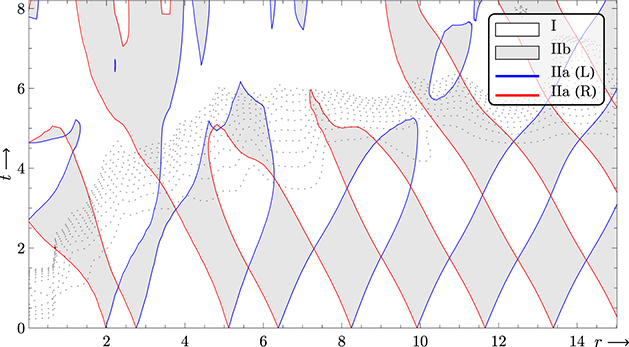
Figure 15. Causal diagram for the bimetric spherical cloud near r = 0.
Download figure:
Standard image High-resolution image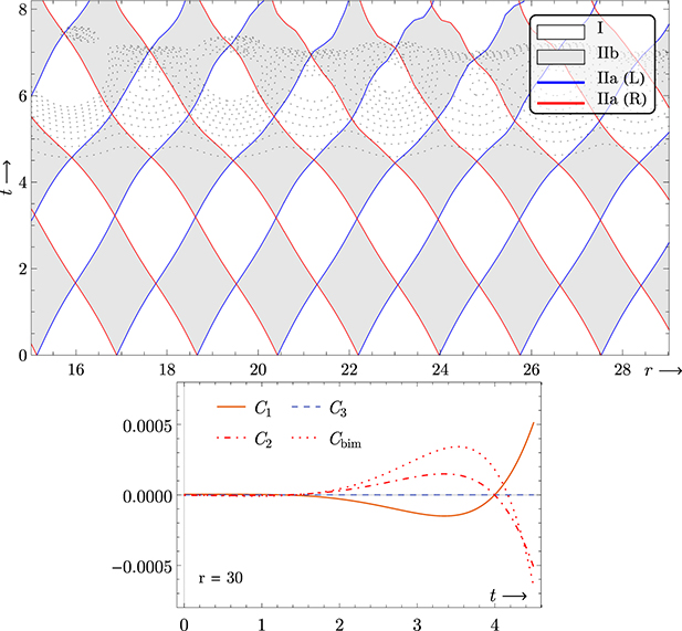
Figure 16. Top: causal diagram for the bimetric spherical cloud at large radii. Bottom: the vertical slice of the constraint violations at r = 30.
Download figure:
Standard image High-resolution imageFinally, we have performed several thousands of simulations for different parameter values, and the earlier shown examples are typical. All the solutions show the time-dependent nonbidiagonality in the dynamics of the two metrics represented by the interwoven and oscillating null cones. An important observation is that the pure bimetric spherical clouds (vacuum solutions) share the same property: they are generically nonbidiagonal and nonstationary; an example is shown in figure 17. The pure bimetric spherical clouds contradict the bimetric analogue of Birkhoff’s theorem [60–62], which is compliant with [63].
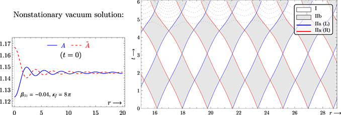
Figure 17. A bimetric spherical cloud for the same parameters as earlier but without matter,  . This is a bimetric nonstationary spherically symmetric solution in vacuum.
Download figure:
Standard image High-resolution image3.3. Gravitational collapse
The simulations are not long enough to shed light on the end point of gravitational collapse. Nevertheless, the present numerical experiments show that the collapse of the dust cloud follows the pattern from the reference GR solution, showing no instabilities. A physically realistic solution is illustrated in figure 18, where the initial data are close to GR and κf ≫ κg = 8π. The time variation of the Lagrange shells is shown in panel (b); the plot is almost the same as in figure 5 (the plots can be compared since the evolution of the time gauge are similar for the two solutions for t < 7).
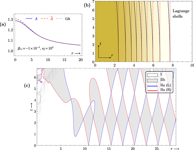
Figure 18. (a) A bimetric spherical cloud where the initial data are close to the reference GR solution. (b) The gravitational collapse follows the same pattern as in figure 5. The vertical dotted lines indicate the initial positions of the Lagrange shells. (c) Although A ≈ AGR, the causal diagram shows the oscillations in the metric fields. The solution is trustworthy for t < 7 and r > 5.
Download figure:
Standard image High-resolution imageThe stress–energy contributions coming from the matter, ρm, and the bimetric potential, ρb, are shown in figures 19(a) and (b). These contributions enter the constraint equations (2.11a) and (2.20a). In the GR limit, ρb is more than 103 times smaller than ρm, due to small β(n)-parameters. For comparison, figure 19(c) shows a large contribution from the bimetric potential when the initial data are far from GR (as in figure 2).
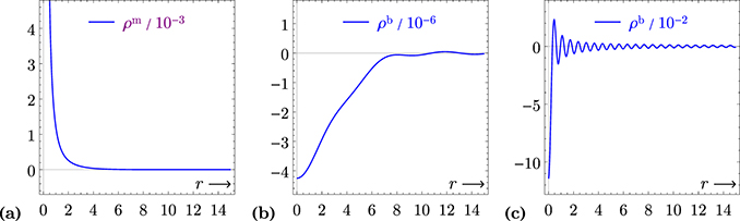
Figure 19. The initial stress–energy contributions coming from: (a) the matter ρm, (b) the bimetric potential ρb in the GR limit for β(1) = −10−4, κf = 104, and (c) the bimetric potential ρb when the initial data are far from GR, having β(1) = −1 and κf = 8π.
Download figure:
Standard image High-resolution image4. Discussion and outlook
In this work, we have:
- (a)Presented a method for solving the constraint equations in the Hassan–Rosen theory to determine bimetric initial data by deforming the existing GR initial data,
- (b)Obtained the Lane–Emden-like equations for the bimetric initial data specifically assuming the conformally flat spatial metrics at the moment of time symmetry,
- (c)Solved for and analyzed the obtained initial data,
- (d)Evolved the initial data using a new numerical code for bimetric relativity.
The results once again point out the importance of nonbidiagonality in the dynamics of the two metrics. The authors in [64] showed that to have dynamically stable solutions, nondiagonal metric elements are needed. Moreover, [65] concludes that considering static black hole solutions in the HR theory is insufficient and that a full dynamical treatment needs to be performed in order to investigate the end point of gravitational collapse. Finally, even in the absence of external matter sources, the bimetric solutions are essentially nonbidiagonal and nonstationary; hence, our results disprove the analogue version of Birkhoff’s theorem for bimetric theory, which is compatible with the findings in [63].
The initial data for bimetric spherical clouds requires negative β(n)-parameters because of the boundary conditions that are imposed on the constraint equation (2.20a) (see figure 7). This would correspond to an imaginary Fierz–Pauli mass obtained from the spectrum of linearized mass eigenstates on the proportional backgrounds [5, 29, 66]. However, the bimetric spherical clouds are nonproportional solutions in a strong-field regime with the initial conditions that assume conformal flatness. In addition, we are more restrictive on the choice of β(0) and β(4) in (2.21) than needed to define the Fierz–Pauli mass, which could affect the conclusions on its sign. This suggests that the properties of the bimetric parameter space should be further investigated.
Similarly to GR, the PDE system of evolution equations is ill-posed in general since it is in standard 3 + 1 form. A future goal is to obtain a long term development of the initial data. For this purpose, the covariant BSSN formalism is established in [15], and various gauge conditions specific to bimetric relativity are investigated in [21]. The hyperbolicity of the reduced bimetric field equations is discussed in more detail in [15]. Work in progress deals with the implementation of BSSN in bim-solver to obtain stable numerical simulations in spherical symmetry.
Finally, we comment on a possibility to extend the present method to construct initial data for non-spherically symmetric spacetimes. In spherical symmetry, the spacetime dimension is effectively 1 + 1, so the square root is parametrized by a scalar p. In the case of axial symmetry, the effective dimension is 1 + 2, which results in a complicated expression for a two-dimensional vector p. Moreover, the closed form of the ratio of lapses is not known for this case, so one of the lapses must be numerically solved during the evolution.
Acknowledgments
We would like to thank Giovanni Camelio for a careful reading of the manuscript.
Appendix A.: Bimetric causal diagrams
Here we give an overview of the procedure [31] how to plot a bimetric causal diagram in spherical symmetry. Consider two metrics given in (1.1). Let rL and rR be the coordinates of the g null cone, and similarly  and
and  the coordinates of the f null cone, both cut at ∂/∂t in the tangent space (these coordinates can be obtained by setting g, f, dΩ = 0, dt = 1, and then solving for dr),

Then, the causal type can be determined from the following two distances using table A.1,

The causal regions can be shown by plotting the product LΔRΔ, in which case type I regions have LΔRΔ < 0, type IIb regions LΔRΔ > 0, and type IIa regions have LΔRΔ = 0 (type I if it is a double zero). An example for the solution from figure 4 is shown in figure 20.
Table A.1. Causal type discrimination based on LΔ and RΔ.
| LΔ | RΔ | LΔRΔ | Causal type | Comment |
|---|---|---|---|---|
| <0 | <0 | >0 | Type IIb | g left of f |
| <0 | =0 | =0 | Type IIa (R) | right null direction in common |
| <0 | >0 | <0 | Type I | f inside g |
| =0 | <0 | =0 | Type IIa (L) | left null direction in common |
| =0 | =0 | =0 | Type I | double null direction in common |
| =0 | >0 | =0 | Type IIa (L) | left null direction in common |
| >0 | <0 | <0 | Type I | g inside f |
| >0 | =0 | =0 | Type IIa (R) | right null direction in common |
| >0 | >0 | >0 | Type IIb | f left of g |
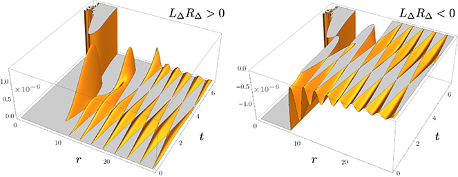
Figure 20. Discriminant LΔRΔ for the bimetric solution similar to the one in figure 4.
Download figure:
Standard image High-resolution imageNote that LΔ and RΔ are smooth functions, smoothly deformed by the coordinate transformations. Hence, topological features (e.g., which regions are adjacent to each other) can not be removed. Finally, the causal types can be tracked along any curve (or surface) as shown in figure 21.
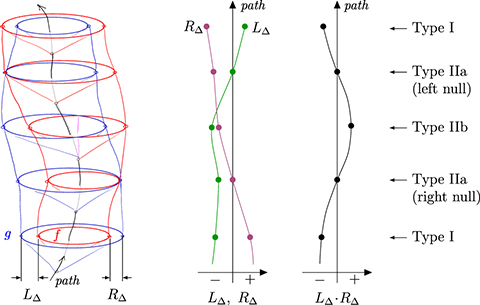
Figure 21. Tracking the causal type along an arbitrary path.
Download figure:
Standard image High-resolution imageAppendix B.: Evolution equations
The evolution equations for the spatial metrics are,


The evolution equations for the extrinsic curvatures are,

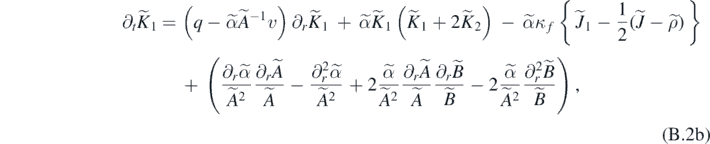

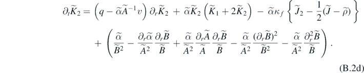
The above set of equations is in each sector equivalent to the GR case [6].
These equations are subject to the regularization procedure described in [9, 43, 51, 52]. There are two types of regularity conditions that must be satisfied. First, the parity which comes from symmetry considerations. Spherical symmetry implies that a reflection in the radial coordinate leaves metrics unchanged. After reflecting r → −r, we see that the lapses, the spatial metric components, and the corresponding components of the extrinsic curvature must be even functions of r, while the shift vector must be odd. Beside the parity, the extra regularity conditions require that the manifold must be locally flat at the origin. The regularization is done in several steps (done in both sectors):
- (a)Redefine B → Br (and similarly
 ),
), - (b)Introduce:Dα ≔ ∂r log α, DA ≔ ∂r log A, DB ≔ ∂r log B,σ = (A − B)/r, and KΔ = (K1 − K2)/r,
- (c)Find the evolution equation for these variables,
- (d)Evolve these variables imposing the odd parity conditions.

The regularized equations are too long to write down here; they are relegated to an ancillary file, which can be found on arXiv [53].
Footnotes
- 2
Before coupling matter, the bimetric field equations exhibit duality under the exchange of metrics. The metric sector where the standard model fields are coupled define the physical metric, in the paper selected to be g. Of course, one can also couple another independent matter to f, but this matter will only interact indirectly to the physical matter. Coupling the same matter to both metrics reintroduces the ghost modes (see, e.g., [29]).
- 3
The l2-norm is used to measure distance in the function space of solutions (see, e.g., [32]).