Abstract
In this work we study the long-lived post-merger gravitational wave signature of a boson-star binary coalescence. We use full numerical relativity to simulate the post-merger and track the gravitational afterglow over an extended period of time. We implement recent innovations for the binary initial data, which significantly reduce spurious initial excitations of the scalar field profiles, as well as a measure for the angular momentum that allows us to track the total momentum of the spatial volume, including the curvature contribution. Crucially, we find the afterglow to last much longer than the spin-down timescale. This prolonged gravitational wave afterglow provides a characteristic signal that may distinguish it from other astrophysical sources.
Original content from this work may be used under the terms of the Creative Commons Attribution 4.0 license. Any further distribution of this work must maintain attribution to the author(s) and the title of the work, journal citation and DOI.
1. Introduction
Gravitational waves (GWs) were first predicted by Einstein in 1916 as a consequence of general relativity. Their recent detection by the LIGO and Virgo observatories has opened up a new window on the Universe. This window has led to new probes of the nature of black holes (BHs) and to a wealth of astrophysical findings, challenging our understanding of stellar evolution and binary population models [1–4]. However, one of the most exciting and as yet unrealized prospects is to use GWs to shed light on the nature of the dark matter (DM) component of the Universe’s energy budget. In the absence of direct couplings between dark and baryonic matter, gravitational interactions will be the only way to probe fundamental characteristics of DM—i.e. mass, spin and strength of self-interactions. With weakly interacting massive particles proving elusive in direct detection experiments, there has been a resurgence in the interest of other DM candidates, particularly those with low masses ( eV) and bosonic in nature. Promising alternatives of this type include the QCD axion, axion-like particles motivated by string theory compactifications, and ‘dark photons’ [5–14].
These bosonic distributions may condense, for example from localized overdensities [15], into gravitationally bound compact objects, which are referred to as boson stars (BSs) [16–27]. Stationary equilibrium solutions of this type have been found for different types of bosons, including scalars [23, 28–53], vector fields [54–67] or higher-spin fields [68].
Binary coalescences involving BSs represent a promising channel to observationally identify or constrain their populations. Their potentially high compactness implies that mergers can generate GWs detectable with present GW observatories. Most present work in the literature on BSs focusses on the GW signatures generated during the pre-merger infall or inspiral [69–73] and during the merger phase itself [21, 28, 74–89]; these are, of course, the regimes of most notable interest in the GW observation of neutron-star and black-hole binary coalescences. The main focus of our work, however, is the long-lived post-merger GW emission or afterglow resulting from the merger of two BSs into a single compact but horizon-free remnant; for first explorations of BS coalescences including the relaxation into a non-rotating BS or a hairy BH see [75, 79, 82]. First indications of such an afterglow were noted in [78] in the case of a head-on collision resulting in a highly perturbed BS. Here, we demonstrate that this afterglow can be very long lived, with barely any decay in amplitude following a transient burst during the merger phase itself. The characteristics of this post-merger afterglow contrast sharply with the corresponding GW signatures of most BH or NS mergers, which, if resulting in BH formation, are dominated by the exponential quasi-normal ringdown.
We illustrate and explore in detail the gravitational afterglow of BSs for the case of the inspiral and merger of two equal-mass BSs in a collision with a non-zero impact parameter. For the moderate compactness of the initial binary constituents chosen in our simulations, the final state of the collision is a highly perturbed BS with decreasing spin. Crucially, this spin-down occurs on a time scale much longer than a single GW oscillation time period. The associated long-lived GW afterglow may exhibit information about the post-merger dynamics of such systems. In particular, we find an intriguing correlation between the phases of different GW multipoles and the dynamical spin amplitude.
The results of this paper suggest that using standard merger templates consisting mostly of the inspiral and merger contributions may be insufficient to capture fundamental dynamics of a boson-star merger event. Rather, comprehensive BS searches likely require extended waveform templates which also capture the rich post-merger GW afterglow phenomenology.
This paper is structured as follows: In section 2 we briefly summarize our computational framework, list the parameters of our initial configurations and the grid setups employed in their time evolution, and introduce the diagnostics specific to our simulations. In section 3, we list the key features of the post-merger remnant. The corresponding GW signal is discussed in more detail in section 4 and we conclude in section 5. Technical details of the numerical methodology, the calculation of angular momentum, and the estimate of numerical uncertainties are relegated to appendices  , and we express the gravitational constant in terms of the Planck mass
  . Unless specified otherwise, Latin indices run from 1 to 3 while Greek ones run from 0 to 3.
2. Simulation set-up
Throughout this work, we model BSs as a complex scalar field minimally coupled to the gravitational sector of a Lorentzian manifold with metric  . The corresponding Lagrangian is given by the Einstein–Hilbert action plus a matter term,


with the potential function for a non-interacting scalar of mass m,

This choice of potential results in BS solutions that are referred to as mini-boson stars [32, 90, 91]. Our construction of boson-star binary initial data can loosely be summarized in the following three steps.
- (a)Generate a stationary, non-rotating solution for a single BS.
- (b)Apply a Lorentz boost to obtain a single star with linear momentum.
- (c)
Most of our results are obtained from simulating a grazing collision of two stable BSs, each with mass
6
 and initial velocity
  .
.
The stars are initially located  apart in the x direction and also offset by an impact parameter
  perpendicular to this axis; it is through this offset (rather than a velocity component off the x direction) that the binary is endowed with initial orbital angular momentum. The Newtonian point-particle estimate for the angular momentum of this configuration,

agrees remarkably well with the relativistic measurement which only deviates by 1.1%. A summary of this binary’s initial data together with the main parameters of the numerical setup are given in table 1. We have simulated numerous other binary configurations—different BS masses, initial velocities v and impact parameters b—that display qualitatively the same behavior. The main features of the binary dynamics that we will report in the following are thus not a consequence of any fine tuning of initial data.
Table 1. Overview of the simulations. Here, M is the individual mass of each BS, vx
the initial velocity, b the impact parameter,  the initial distance in the x direction, b the vertical offset or impact parameter and N is the number of cells on the coarsest AMR Level (which sets the resolution of the respective runs). We allow for seven extra refinement levels. The data associated with these runs can be found here: https://github.com/ThomasHelfer/BosonStarAfterglow.
| Run | N |

|

| vx |

| |
|---|---|---|---|---|---|---|
| Low | 1 | 256 | 80 | 8 | 0.1 | 0.395(0) |
| Medium | 2 | 320 | 80 | 8 | 0.1 | 0.395(0) |
| High | 3 | 384 | 80 | 8 | 0.1 | 0.395(0) |
| Ultra-high | 4 | 448 | 80 | 8 | 0.1 | 0.395(0) |
For all simulations, we use a square box of width  , employing the adaptive mesh refinement (AMR) capabilities of GRChombo [93–95]. Besides the standard computation of the Newman-Penrose scalar whose implementation in GRChombo is described in detail in [93], we compute in our simulations two diagnostic quantities specific to the BS systems under study.
First, we introduce the mass measure

where  is the energy density as measured by observers moving along the normal vector nµ
to the spatial hypersurfaces. The second is a time dependent measure
is the energy density as measured by observers moving along the normal vector nµ
to the spatial hypersurfaces. The second is a time dependent measure  , defined in equation (B10), for the angular momentum contained inside a specified volume V. This quantity is obtained by adding to the initial angular momentum the time integrated rate of change due to the source of momentum that crucially includes contributions from the spacetime dynamics; the details for computing this quantity
  are given in appendix
3. The merger remnant
When colliding two BSs with angular momentum, we expect one of the following outcomes:
- (a)
- (b)
- (c)
- (d)Total dispersion of all matter.
For sufficiently small compactness of the progenitors the merger does not form a BH. While we have observed black-hole formation in some of our calibration runs starting with more compact BSs, in the remainder of this paper we focus on the scenario where the merger results in a compact bosonic configuration without a horizon as shown in figure 1. The scalar-amplitude profiles in this figure (nor at any other times during the evolution) display no signs of a toroidal structure and we therefore interpret the merger outcome as a perturbed non-spinning BS corresponding to the second item in the above list; see also [79, 80].
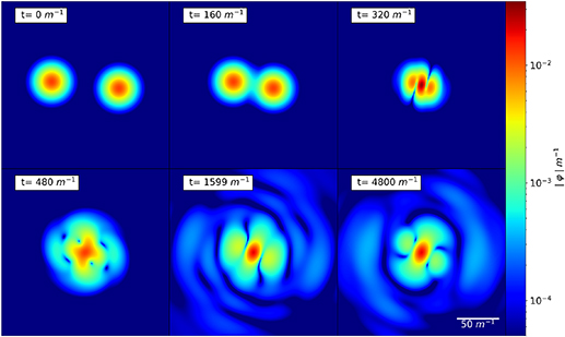
Figure 1. Snapshots of the scalar field amplitude  in the orbital plane for a grazing collision of two BSs of equal mass
  starting with initial horizontal distance
  , impact parameter
  (vertical center to center distance) and initial velocity
  in the x (horizontal) direction. A video of the merger can be found at https://youtu.be/JE5FRG7kgvU.
Download figure:
Standard image High-resolution imageIn figure 2, we display the angular momentum  of the BS configuration inside a coordinate sphere of radius
  throughout inspiral, merger and the afterglow phase. Up to the time of merger around
  , the angular momentum remains approximately constant before rapidly decreasing in the post-merger phase. To leading order, the tail of the resulting curve
  is approximated by an exponential decay with half-life
  , as obtained from an exponential fit to the data of Run 2 starting at
  .
.
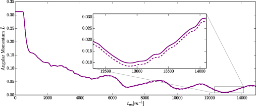
Figure 2. Angular momentum of the scalar field: We show the angular momentum  (see definition in equation (B10)) inside a coordinate sphere of radius
  as a function of time. We compute
  in two ways, (i) via integrating the outgoing flux—solid lines (see equation (B4)) – and (ii) as a volume-integral—dotted lines. This was plotted using run 2 of table 1.
Download figure:
Standard image High-resolution imageTranslated into SI units, the half-life is

For a scalar mass  eV, for example, the dominant frequency of the
  , m = 0 signal falls into the most sensitive region of the LISA noise curve (see equation (7) below) and we obtain a half-life of
  . For scalar masses in or above this regime, this implies that a delayed formation of a BH, should it occur, will result in a BH with negligible spin. With regard to the possibility of the formation of a black-hole population through isolated BS progenitors [42, 43], this implies that spinning BHs are unlikely to have formed this way unless the BS progenitors are composed of ultra light scalar particles. More quantitatively, we see from equation (6), that astrophysically large decay times for the angular momentum of order
  require ultra light scalars with mass
7
require ultra light scalars with mass
7
 .
.
The rapid drop in the angular momentum of rotating scalar soliton stars has been noticed as early as the mid 1980s [35, 36], but we note that the post-merger evolution of our  , besides an approximately exponential drop, also exhibits significant oscillations on a time scale of about 2000 m−1. We conjecture that these oscillations arise from the complex dynamics of the post-merger remnant and may carry memory of its formation process.
We also observe significant oscillations in the time evolution of the merger remnant’s mass M as defined in equation (5). As demonstrated in figure 3, however, the mass evolution differs significantly from that of the angular momentum. First, the mass gradually levels off at  or
or  % of the initial mass instead of decaying over time. Second, the oscillations occur on a much shorter time scale.
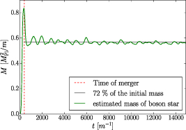
Figure 3. The estimated mass using equation (5) contained inside a box Ω with side length  as computed for the ‘medium’ resolution run 2 of table 1. Since the BSs are not initially inside this box, the mass at t = 0 is close to zero. The small fluctuations after merger are due to the gauge-dependence of the measure.
Download figure:
Standard image High-resolution image4. GW signal
We now turn our attention to the GW signal generated by the BS coalescence. We find this signal to be dominated by the  and
and  quadrupole modes which are displayed in figure 4 for Run 2 using an extraction radius
  . The large burst around merger at
  (see the upper left inset of the figure) closely resembles the corresponding features regularly seen in the merger of black-hole binaries. The ensuing long-lived, semi-regular radiation clearly visible with barely any signs of diminuition up to the end of our simulation, however, drastically differs from the familiar ringdown of a merged BH. This afterglow signal is the main result of our study. We emphasize that this signal is well resolved (rather than merely displaying numerical noise), and also persists with negligible variation under changes in the numerical resolution of our grid. As discussed in more detail in
  signal at about
  during the afterglow phase with most of this error budget being due to the finite extraction radius. The GW signals of the higher-resolution Runs 3 and 4, if added to figure 4, would almost overlap with that shown in the figure for Run
8
2; cf also figure 5 below.
during the afterglow phase with most of this error budget being due to the finite extraction radius. The GW signals of the higher-resolution Runs 3 and 4, if added to figure 4, would almost overlap with that shown in the figure for Run
8
2; cf also figure 5 below.
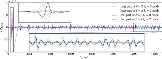
Figure 4. GW afterglow emission from the collision of two BSs with non-zero impact parameter (‘medium’ run in table 1). The Weyl scalar Ψ4 is extracted at  and we only show the dominant
  modes. The
  vanishes identically due to symmetry. There is a large initial burst at merger (first zoom-in box), followed by a long, but irregular signal produced by the excited remnant BS. A video of the merger can be found at https://youtu.be/JE5FRG7kgvU.
Download figure:
Standard image High-resolution image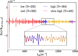
Figure 5. Convergence: We display the  multipole of the GW signal obtained for four different resolutions corresponding to runs 1 to 4 in table 1. A quantitative analysis yields overall convergence at first order.
Download figure:
Standard image High-resolution imageThe afterglow signal (without the prodigious merger burst) is also shown in figure 6 together with its Fourier spectrum. The frequency spectrum demonstrates contributions on many time scales, but also reveals a narrow dominant peak at  which, translated into SI units, can be written as

Both the time- and frequency-domain signals exhibit signature of beating effects: the amplitude of the rapid oscillations itself undergoes a modulation at lower frequency.
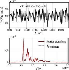
Figure 6. Time domain signal and Fourier transform of the  mode of
  : We perform a Fourier transformation of the tail of the GW signal of the ‘medium’ resolution run in table 1. We find excellent agreement between the displayed spectrum for the
  mode and the corresponding Fourier transform of the
  mode; in particular, both yield the same peak frequency.
Download figure:
Standard image High-resolution imageThe prolonged afterglow furthermore accumulates a non-negligible amount of energy emitted in GWs. By the end of our simulation at  , the radiated energy computed according to equation (C1) including infall and merger has reached
  of the initial mass, corresponding to an average rate of
  (see dotted line in figure 7). The radiated energy and power are shown as functions of time in figure 7 and clearly show an approximately linear increase in
  during the afterglow phase. This significant amount of post-merger GW emission in itself is a striking signature of exotic binary merger progenitors that distinguishes them from BH binaries devoid of significant post-merger radiation beyond the quasi-normal ringdown. By using windowing of the GW signal, we find that the rate of radiation in the afterglow (excluding the merger peak) decreases by about
  over the course of the simulation. Note that the decay in GWs is much more protracted than the drop in the angular momentum displayed in figure 2. Clearly, the system loses angular momentum much more rapidly than energy.
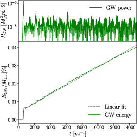
Figure 7. Radiated GW energy over time: We calculate the energy and power radiated in GWs from the ‘medium’ resolution run of table 1. We observe no significant reduction in the GW radiation over the simulation time, allowing us to estimate a lower bound on the half-life of the signal.
Download figure:
Standard image High-resolution imageA more subtle feature in the post-merger signal is revealed in the multi-polar decomposition of the quadrupole signal; more specifically in the relative position of the local extrema in the  and
and  modes. As exhibited by the upper left inset of figure 4, the amplitudes of the
  and
and  modes are almost exactly in anti-phase around merger and remain so in the early afterglow around
  . At late times
  , however, the two modes are almost synchronized with their extrema in good overlap. The timing of this synchronization coincides remarkably well with the drop in angular momentum shown in figure 2 and we hypothesize the two effects are causally related. This would imply a concrete observational signature of the BS angular momentum in the emitted GW afterglow signal.
In physical terms, the GW afterglow is a direct consequence of the the presence of matter around the compact merger remnant and the resulting complex matter dynamics following the violent merger. A qualitatively similar behavior may arise in the merger of neutron stars provided these do not promptly merge into a BH. Two key differences between neutron-star and boson-star binaries, however, may aid considerably in the distinction between neutron-star and BS signals. The first consists in the extremely long-lived nature of the BS afterglow which we anticipate will last for much longer times than are presently within grasp of our numerical studies; cf again figure 4 and the barely perceptible drop in the GW signal. The second fundamental discriminator arises from the scale-free nature of the BS spacetimes; the scalar mass parameter m appears as a characteristic scale in all dimensional variables of the GW analysis. While NS masses are restricted to be below the Chandrasekhar limit of about  , BSs may theoretically exist across the entire mass spectrum and barring for a remarkable coincidence in the scalar mass value, will be distinguishable from their neutron-star counter parts by the frequency regime of their GW emission. Put the other way round, comprehensive observational searches for GW signatures from BSs require scanning over a wide range of frequencies using vastly different detectors such as LIGO-Virgo-KAGRA, LISA, third-generation detectors but also high frequency GW observatories presently under development [103, 104].
5. Conclusion
In this paper, we have shown that the inspiral and coalescence of BS binaries into a non-BH remnant can produce a long-lasting GW afterglow. This signature is salient, and markedly differs in duration and—possibly—also frequency from the GW signatures of more traditional astrophysical compact object mergers; it thus represents a distinct detection channel for exotic compact objects in compact-binary-coalescence and continuous-GW searches [105–112].
There are several implications resulting from our findings. In terms of search strategies, as mentioned in the introduction, these signatures are likely to be missed if we focus exclusively on constructing pre-merger inspiral and merger waveform templates. The systematic construction of waveform templates for post-merger signatures of this type of binaries is in its infancy at present and an immediate challenge for further work consists in identifying an effective parameterization of the GW signatures. Our results furthermore demonstrate an efficient loss of angular momentum in BS mergers resulting in a horizon-less remnant, consistent with previous studies noticing that the spin of rotating BSs decays with a fairly short half-life of  [113]. We also observe a remarkable correlation between the BS remnant’s spin-down in figure 2 with a gradual synchronization of the local extrema in the GW amplitudes of the
  and
and  modes; from near anti-alignment of the peaks around merger and shortly thereafter, the extrema gradually shift into approximate overlap over a time interval
  (see figure 4), coinciding exactly with the time during which the angular momentum drops to a negligible level. We tentatively conclude that through this synchronization, the GW afterglow carries important information about the remnant’s dynamical evolution.
Given the extraordinary length of the afterglow signal, one would expect the radiation from numerous BS merger events—if they occur—to result in a stochastic background. Such a background could be searched for additionally to that expected from more traditional binary mergers [114]. Evidently, more exploration of the underlying BS parameter space and the resulting afterglow phenomenology will be required to relate theoretical estimates of the GW background to hypothesized BS populations. We reiterate, however, that nothing about our BS configurations has been fine-tuned, so that we expect the afterglow to be a rather generic feature of BS coalescences as long as these do not promptly form a BH.
Acknowledgment
We thank Caio Macedo and Emanuele Berti for helpful discussion. T H is supported by NSF Grant Nos. AST-2006538, PHY-2207502, PHY-090003 and PHY20043, and NASA Grant Nos. 19-ATP19-0051, 20-LPS20- 0011 and 21-ATP21-0010. This research project was conducted using computational resources at the Maryland Advanced Research Computing Center (MARCC). K C acknowledges funding from the European Research Council (ERC) under the European Unions Horizon 2020 research and innovation programme (Grant Agreement No. 693024), and an STFC Ernest Rutherford Fellowship project reference ST/V003240/1. This work has been supported by STFC Research Grant No. ST/V005669/1 ‘Probing Fundamental Physics with Gravitational-Wave Observations’. R C and T E are supported by the Centre for Doctoral Training (CDT) at the University of Cambridge funded through STFC. We acknowledge the Cambridge Service for Data Driven Discovery (CSD3) system at the University of Cambridge and Cosma 7 and 8 of Durham University through STFC capital Grant Nos. ST/P002307/1 and ST/R002452/1, and STFC operations Grant No. ST/R00689X/1. The authors acknowledge the Texas Advanced Computing Center (TACC) at The University of Texas at Austin for providing HPC resources that have contributed to the research results reported within this paper [115]. The authors would like to acknowledge networking support by the GWverse COST Action CA16104, ‘Black holes, gravitational waves and fundamental physics.’. This research made use of the following software: SciPy [116], Matplotlib [117], NumPy [118] and yt [119].
Data availability statement
The data that support the findings of this study are openly available at the following URL/DOI: https://github.com/ThomasHelfer/BosonStarAfterglow.
Appendix A: Numerical methodology
The simulations of this work have been performed with GRChombo, a multipurpose numerical relativity code [93–95] which evolves the CCZ4 [120, 121] formulation of the Einstein equation. The four-dimensional spacetime metric is decomposed into a spatial metric on a three-dimensional spatial hypersurface, γij , and an extrinsic curvature Kij , which are both evolved along a chosen local time coordinate t. The line element of the decomposition is

where α and βi denote the lapse function and shift vector. For more details about the grchombo code and the system of evolution equations see [93, 94].
The matter part of the Lagrangian is given by

whose variation with respect to the scalar field gives the evolution equation

We implement this equation as a first-order system in terms of the CCZ4 variables in the form


The energy-momentum tensor is

and its space-time projections, defined by

are



These are the expressions for the matter terms that source the evolution of the spacetime geometry according to the evolution equations (13)–(18) in [93].
Appendix B: Angular momentum measure
Conserved quantities in general relativity are associated with isometries of the spacetime manifold. In particular, if a spacetime conserves energy, then there must exist a time-like Killing vector field ξ . A classic example is that of the Kerr vacuum solution. On the other hand, in a less symmetric spacetime like that of a black-hole merger, such a Killing vector field does not usually exist except in the asymptotically flat region. In this section we define a diagnostic quantity for the angular momentum that does not require a Killing vector, but merely a vector field to generate a measure that converges to the classical angular momentum definition in the flat-spacetime limit.
In order to define such a measure in a precise manner, we will follow the work of [122, 123] where readers will also find more details of the calculations.
We start by defining, based on our Cartesian coordinates, the azimuthal vector

We next define the angular angular momentum

with the volume element  on the spatial hypersurface Σ, which in our case is a sphere of finite radius, and

where  is the azimuthal component of the mixed space-time projection Si
given by equation (A9). We also integrate the angular momentum flux density
is the azimuthal component of the mixed space-time projection Si
given by equation (A9). We also integrate the angular momentum flux density  through
  , to get the total angular momentum flux

Here  is the induced volume element on
  and the flux density is

where
β
is the shift vector where  and with
  the radial unit vector.
If  is a Killing vector the rate of change of the momentum within a given volume Σ will be equal to the momentum flux through the boundary, i.e.

However, in general dynamical spacetimes, we do not have such a Killing vector and angular momentum is not conserved in this simple manner. Instead, we obtain a further term representing curvature contributions on the right-hand side of equation (B6) which effectively acts as a further source or sink of momentum for the matter [122, 123]. This term is given by

where the momentum source density  expressed in terms of the 3+1 variables is

for a spacelike vector ξ . The corresponding term for a timelike vector ξ is given (see equation (19) in [123]). We can thus generalize equation (B6) to the exact conservation law

a schematic overview of the different contributions to this balance law is shown in figure 8. In the flat-space limit  , so that find that
  and we recover equation (B6) as expected given the symmetry of flat spacetime.
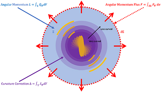
Figure 8. Schematic representation of the angular momentum measure: We illustrate the origin of the different quantities appearing in the conservation equation (B9): The angular momentum L, the angular momentum flux F and the curvature correction Δ. Recall that the post-merger configuration does not have a toroidal structure as would be expected for the spinning BS model of [96, 97], but is more bar-like in shape.
Download figure:
Standard image High-resolution imageIn our simulations we introduce the adjusted angular momentum defined as

which obeys the equation

We can then define a relative measure for the error in the conservation of angular momentum as

The resulting error measured for our BS binary using the four different resolutions is shown in figure 9 and exhibits clear convergence toward the expected limit of zero.
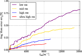
Figure 9. Angular momentum error: We numerically verify the conservation equation (B9) for the simulations with parameters given in table 1. In the continuum limit this quantity becomes zero. The colored curves obtained for different resolutions demonstrate conservation with excellent accuracy of about  error after 16 000
 and exhibit convergence to the zero continuum limit.
Download figure:
Standard image High-resolution imageWe reiterate that this angular momentum measure is a local quantity that obeys a rigorous conservation law given by equation (B11) for any chosen volume. Its calculation does therefore not require extrapolation to infinity (as is needed, for example, for the calculation of the GW signal) nor even asymptotic flatness of the underlying spacetime. However, to relate it to a more physical measure, such as the ADM angular momentum of the spacetime, we do require such conditions. Also note that for matter fields decaying to zero on the surface of Σ the quantity  (but not L) is constant in time for a general spacetime.
In practice, we monitor the conservation of  as follows. We calculate our angular momentum measure by integrating (i) the angular momentum (see equation (B10)), and (ii) integrating the flux F (see equation (B4)) over time; we set the integration constant equal to
  . Having thus obtained two measures for the same quantity allows us to estimate the uncertainty by taking the difference between the two; see figure 9 for the evolution of the error. Using the final value of
  obtained for Run 2 (see table 1) inside the volume of a coordinate sphere of coordinate radius
  , we estimate the final spin of the merged BS as
Appendix C: Numerical accuracy
GRChombo evolves the CCZ4 equations using the method of lines with a standard fourth-order Runge-Kutta method (RK4) and for the spatial discretization, we use fourth order centered stencils. To mitigate spurious modes from the AMR, we are using N = 3 Kreiss-Oliger dissipation. More details about the numerical methods used in GRChombo can be found in [93].
To assess the accuracy of our results we have performed simulations with four different resolution given, in terms of the number of points in each direction on the coarsest level, by  , all for a box width of
  ). As demonstrated in figure 5, the individual wave signals obtained for this range of resolution are in excellent agreement. More quantitatively, we observe convergence at about 1st order convergence using the four resolutions for the
  mode of
  . Additionally, we estimate the discretization and error from the finite extraction region in
  and we find that the latter dominates, causing a ∼7% error.
To calculate the energy (see figure 7) we used the the  modes and using the equation for the power

where we apply an 5th order Butterworth high-pass filter (using the scipy implementation [116]) on the integral  . As otherwise accumulating numerical error causes a drift in the Energy over time. We estimate the error, similarly as for
  , using both the discretisation error as well as the error from the finite extraction radius. For the discretization error we use Richardson extrapolation assuming 1st order convergence to estimate the error. Similarly as before, we find that the mostly the error in the finite extraction radius dominates, giving us the value
  .
.
Lastly to calculate the average rate of emission, we simply perform a linear fit over the whole Energy over time signal of the largest radius of the ‘medium’ run (see figure 7). We also perform this fit on a rolling window of  to determine any reduction of radiation over time. Excluding the merger, we find the rate roughly declines by
  over the simulation time.
The GW data and angular momemtum data is available at https://github.com/ThomasHelfer/BosonStarAfterglow.
Footnotes
- 6
This mass is obtained for a central scalar-field amplitude
 and results in a compactness estimate in radial gauge. For comparison the Kaup limit configuration has M = 0.633 and .
 - 7
Note that candidates below
are ruled out as constituting 100% of the DM by structure formation constraints but may still form some proportion of the DM [7]. - 8
Run 2 is our longest simulation and therefore used for most of our analysis.



