Abstract
Kinetic inductance detectors (KIDs) have been proven as reliable systems for astrophysical observations, especially in the millimeter range. Their compact size enables them to optimally fill the focal plane, thus boosting sensitivity. The KIDs Interferometric Spectral Surveyor (KISS) instrument is a millimeter camera that consists of two KID arrays of 316 pixels each coupled to a Martin–Puplett interferometer (MPI). The addition of the MPI grants the KID camera the ability to provide spectral information in the 100 and 300 GHz range. In this paper, we report the main properties of the KISS instrument and its observations. We also describe the calibration and data analysis procedures used. We present a complete model of the observed data including the sky signal and several identified systematics. We have developed a full photometric and spectroscopic data analysis pipeline that translates our observations into science-ready products. We show examples of the results of this pipeline on selected sources: the Moon, Jupiter, and Venus. We note the presence of a deficit of response with respect to expectations and laboratory measurements. The detector's noise level is consistent with values obtained during laboratory measurements, pointing to a suboptimal coupling between the instrument and the telescope as the most probable origin for the problem. This deficit is large enough to prevent the detection of galaxy clusters, which were KISS's main scientific objective. Nevertheless, we have demonstrated the feasibility of this kind of instrument in the prospect of other KID interferometers (such as the CONCERTO instrument). In this regard, we have developed key instrumental technologies such as optical conception, readout electronics, and raw calibration procedures, as well as adapted data analysis procedures.
1. Introduction
The Sunyaev–Zel’dovich effect (SZe; Sunyaev & Zel’dovich 1970, 1972) is one of the most important and thoroughly studied secondary cosmic microwave background (CMB) anisotropies. CMB photons undergo inverse Compton scattering with electrons in hot gas regions, which produces an increase of the photon energy. The electron temperature is particularly high in the intracluster medium within galaxy clusters (GCs), making the SZe a useful probe to detect distant matter structures. Because of the independence of the SZe signal with respect to the redshift at which each GC is located, it has been extensively used for cosmological analysis in the past (e.g., Planck Collaboration et al. 2014, 2016b). Besides this signal, which is normally referred to as the thermal SZe (or tSZe), an additional component of the SZe must be taken into account when the velocity of the GC is not negligible with respect to the CMB reference frame. This component receives the name of kinematic SZe (or kSZe), and it has been studied in less depth (Hand et al. 2012; Planck Collaboration et al. 2016a) because of its lower amplitude (and therefore, more challenging detection).
New physics is available when an accurate description of the SZe beyond its thermal component is achieved, with a special focus on kSZe (Deutsch et al. 2018; Battaglia et al. 2019; Mroczkowski et al. 2019; Münchmeyer et al. 2019). One can rely on their different spectral dependencies in order to separate the two, but precise measurements are required due to the smaller amplitude of kSZe. Therefore, gathering as much data as possible in the millimeter (100–300 GHz) range, where SZe is most important, is mandatory to perform an accurate separation between the two components. Constraining the emission around 217 GHz is especially enlightening, as the tSZe contribution is null at that frequency, so every shift from the expected CMB blackbody distribution will be ascribed to the kSZe.
One way to obtain these data would be to use spectrometers in the millimeter band. Martin–Puplett interferometers (MPIs; Martin & Puplett 1970) allow one to obtain interferometric data produced by a differential signal under a varying optical path difference (OPD). The obtained interferograms are later transformed into the actual spectral energy distribution (SED) from the observed source after running a Fourier transformation. Several other instruments have used Fourier transform spectrometers (FTSs) in the past, both ground-based (e.g., EMIR, Carter et al. 2012; SEPIA, Belitsky et al. 2018) and on board space satellites (e.g., FIRAS, Mather et al. 1999; SPIRE, Griffin et al. 2010). However, for the first time, we propose to couple such a spectrometer with kinetic inductance detectors (KIDs; Zmuidzinas 2012), while most of the previous ones used bolometric or heterodyne receivers. KIDs have been used already in photometric millimeter instruments such as the NIKA and NIKA2 cameras (Monfardini et al. 2010; Adam et al. 2018), both installed at the IRAM 30 m telescope at Pico Veleta. The two have provided extensive information on GCs in the millimeter band for the last 15 yr (e.g., Adam et al. 2014; Perotto et al. 2020).
In order to test this concept and as a test bed for the CONCERTO instrument (CONCERTO Collaboration et al. 2020), we constructed and operated the KIDs Interferometric Spectral Surveyor (KISS) instrument (Fasano et al. 2020a). KISS was installed in the first QUIJOTE (Rubiño-Martín et al. 2010) telescope at the Teide Observatory in Tenerife, from 2018 to 2020. The instrument consisted of a KID camera coupled to the actual warm MPI, which is coupled to the telescope through a series of tailored optics. The data discussed in this work cover a frequency range between 120 and 180 GHz, while data with an additional band between 200 and 300 GHz have been discussed in previous works (e.g., Fasano et al. 2020b). The CONCERTO (CONCERTO Collaboration et al. 2020) instrument followed a similar instrumental configuration while pursuing much finer sensitivity and angular resolution. It was installed in the larger APEX (Güsten et al. 2006) telescope in Chile with a new and customized set of KIDs.
This paper is organized as follows. In Section 2, we introduce the KISS instrument, and in Section 3, we discuss how the raw data are transformed into scientific products. We explain the characteristics and systematics of photometric and spectroscopic data in Sections 4 and 5, respectively. We finally present the scientific results on astrophysical targets in Section 6 and the concluding remarks in Section 7.
2. The KISS Instrument
KISS is a ground-based millimeter Fourier transform spectral imager installed at the first QUIJOTE telescope (Gomez et al. 2010; Gómez-Reñasco et al. 2012), one of the two 2.25 m telescopes of the QUIJOTE experiment at the Teide Observatory. 12 Operations ran from 2018 to 2020. KISS is based on an MPI (Martin & Puplett 1970) coupled to the telescope and to a millimeter camera made of two arrays of KIDs operating in the frequency range from 120 to 180 GHz. KISS has been designed to achieve a typical angular resolution of 7′ at 150 GHz with a field of view (FoV) of 1°. The KISS performance parameters are summarized in Table 1.
Table 1. Basic Performance Parameters of KISS
| Parameter | Value |
|---|---|
| Total number of KIDs | 632 |
| Central frequency (GHz) | 150 |
| Bandwidth (GHz) | 60 |
| Primary mirror diameter (m) | 2.25 |
| FoV (deg) | 1 |
| Sampling frequency (kHz) | 3.816 |
| Beam FWHM 150 GHz (arcmin) | 7 |
| Beam ellipticity, e (arrays A and B) | 0.175–0.275 |
| White-noise level @ 150 GHz | 1.5–2 Hz s1/2 |
| 60–80 mK s1/2 | |
| NEFD @ 150 GHz (Jy s1/2) | 140–180 |
| Calibration factor from | 35.7 ± 2.6 |
| photometry on Jupiter (Hz K−1) | |
| Maximum mirror displacement (mm) | 30 |
| Interferogram rates (Hz) | 7.45 |
| Spectral frequency range (GHz) | 120–180 |
| Results spectral binning (GHz) | 8.33 |
Note. We find a lower value when using the Moon as a calibrator, as explained in Section 6.1.1. The calibration factor obtained from spectral data is also lower than that obtained from photometry, as discussed in Section 5.
Download table as: ASCIITypeset image
2.1. The KISS MPI
An MPI measures the difference between two optical inputs, as all FTSs, but in this case, the beam is split in two with different linear polarization (Martin & Puplett 1970, see Figure 2). This can be done with the use of two initial wire-grid polarizers. After interfering with the MPI, the first half of the beam is focused on the detectors, creating an image of 1° on the sky. The second half of the beam is first defocused from a focused image to a pupil (corresponding to the image of the primary mirror of the telescope) and then collected by the detectors. This accounts for a constant signal over the whole FoV. From the point of view of the spectroscopic measurements, this is equivalent to an initial hardware subtraction of the constant common mode from the atmosphere (which simplifies the offline analysis). Instead of the sky itself, this second, flat input can also be taken from a cold reference, which can be either the detectors themselves by a narcissus effect (i.e., being reflected by a mirror; Howard & Abel 1982) or a cold blackbody at a given tunable temperature. The KISS MPI posed a technological challenge due to the fast scanning speed required to overcome the effects of large-scale atmospheric fluctuations. The control of the systematic errors of such a configuration drives the major requirement for the whole instrument. The MPI must be able to perform continuous 3 cm path interferograms (which give a spectral resolution of about 3 GHz within the band) at a rate of 7.45 Hz 13 to maintain a low sky noise level and sufficient angular sampling on the sky. The fast KID response time permits us to use this method without any loss of information. This requirement also constrains the readout sampling frequency. We found that a few hundred data points for each interferogram are needed in order to preserve all the spectral information from the data in the band of interest. This means that the readout electronics have to operate at a sampling frequency of 3.816 kHz.
These requirements have been studied, and a solution is presented in Figure 1. One of the two roof mirrors is moved by a mechanical-bearing direct-drive linear stage allowing for backward and forward displacement at 3.725 Hz. In order to achieve accurate linear movement and reduce vibration effects, which would significantly increase the noise in the data, we used a flat spiral spring similar to that developed for the Planck HFI 4 K compressor. In this geometry, the flexing movement is produced by arms that connect the inner and outer rings (Fasano et al. 2020a). Flexing allows the planes defined by these rings to move easily with respect to each other by rotation perpendicular to the flexing axis, displacement, or a combination of both.
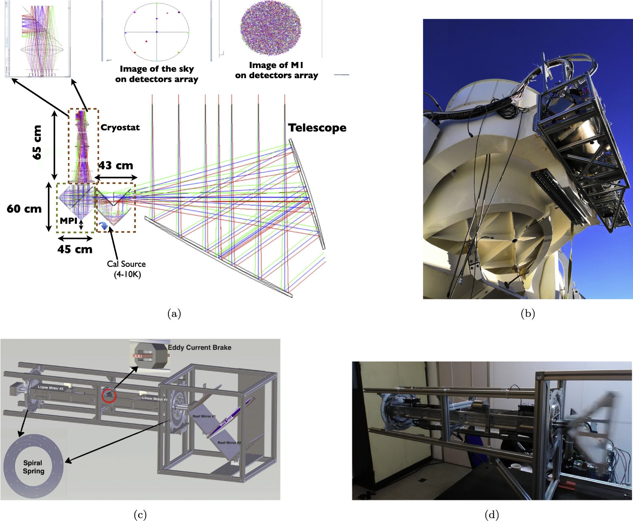
Figure 1. The fast MPI interferometer developed for the KISS experiment. (a) The optical scheme of the KISS instrument. (b) Picture of the instrument installed at the QUIJOTE telescope. (c) and (d) Comparison between a mechanical drawing and the real KISS MPI. It consists of two roof mirrors, one of which can move up to 100 mm with a frequency of 5 Hz.
Download figure:
Standard image High-resolution image2.2. The KISS Camera and Readout Electronics
The KISS camera design is based on the NIKA and NIKA2 cameras (Monfardini et al. 2010; Adam et al. 2018) sharing the same KID technology (Swenson et al. 2010) and readout electronics (Bourrion et al. 2012a, 2012b, 2013, 2016). The optical coupling between the camera, the MPI, and the telescope is ensured by a series of lenses (see Figure 1). The 1° focal plane is fully covered by two arrays of single-polarization aluminum lumped-element KIDs containing 316 pixels each and illuminated by a 45° folded polarizer. Each array has a common optical band of 120–180 GHz. KISS detectors are operated at a temperature of 170 mK, stabilized at 0.5 mK for elevation change. This operation temperature is obtained via a 3He–4He dilution cryostat based on the NIKA camera cryostat (Monfardini et al. 2010), which has been adapted for KISS.
The KISS detectors are instrumented by two (one per array) AMC NIKEL electronic boards (Bourrion et al. 2016). For each array, the KIDs are coupled to a single transmission line and are read simultaneously in the Fourier domain. Variations in the sky signal produce shifts in the KID resonance frequency that are measured by the readout electronics. For each KID, noted k, a frequency tone is injected. The electronic readout monitor then allows recovery of the in-phase (Ik ) and quadrature (Qk ) response of the KID to that input tone. These two quantities can be related to the KID resonance frequency shift. For this, we modulate the frequency tone for each KID and apply the three-point calibration algorithm described in detail in Fasano et al. (2021). As explained later in Section 3, KISS was operated in sky-sky mode for which we expect moderate signal amplitudes and as so in the range of operation of the three-point calibration procedure. If this is not the case, an extra modulation cycle at the end of each scan can be introduced to reconstruct the resonance shape for each detector. This has already been considered in the updated version of the KISS software used in CONCERTO (Hu et al. 2024).
3. Raw Data and Observation Modes
The KISS instrument can be considered as a spectral imager, allowing us to obtain spectral and photometric data simultaneously over the full FoV. For a given scanning strategy, we intend to reconstruct the sky SED for each sky position. As for other MPI-based instruments, SEDs can be reconstructed directly from the Fourier transform of interferograms, as detailed in the following section. These interferograms are produced by displacing the movable roof mirror from a given initial position to the maximum displacement and back to the initial position, as introduced in Section 2. Figure 2 shows a schematic view of the KISS MPI and the interface with the telescope and the KID arrays.
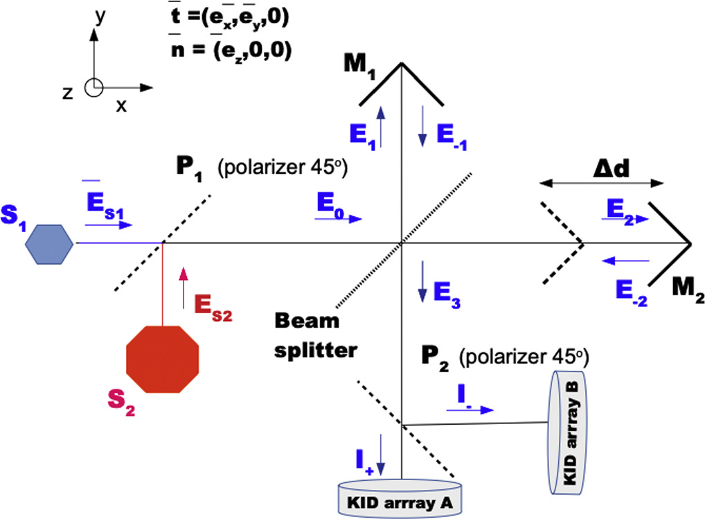
Figure 2. KISS Martin–Puplett schematic view. Input signals S1 and S2 are combined to produce an interference pattern thanks to the displacement of a roof mirror (M2) with respect to a fixed one (M1).
Download figure:
Standard image High-resolution image3.1. Interferograms and Spectral Energy Density
Considering two multichromatic input sky signals, S1(ν) and S2(ν), we can write the total observed intensity in the two detector arrays as

with

where H(ν) and Tatm(ν) represent the KISS frequency transmission and the atmospheric transmission, respectively. The relations between the total observed intensity from Equation (1) and the electrical fields propagating through the instrument (as shown in Figure 2) are detailed in Appendix A. The ± relates to the in-transmission or in-reflection outputs of the MPI corresponding to KID arrays A and B, as shown in Figure 2.
The first term can be considered as the total photometric continuum contribution including both input signals, S1 and S2. The second term can be identified as the spectroscopic measurement. In practice, as discussed above, by moving the roof mirror in the range  to
to  , it is possible to reconstruct the SED of the input signal as the inverse Fourier transform of the interferometric signal,
where  represents the real part.
3.2. Raw Signal Data and Modulation
The raw signal data from the KISS instrument consist of blocks of 1024 points at a sampling rate of 3.816 kHz.
14
For each sample, we register (Ik
, Qk
) for each KID. The readout electronics and MPI motors are synchronized so that the roof mirror does a full forward–backward displacement producing a forward ( ) and a backward (
 ) interferogram within each block. The initial position of the displacement mirror is set so that the zero path difference (ZPD) is well centered with respect to the mirror path. Two lasers allow us to monitor the displacement of the mirror and thus reconstruct the OPD.
In order to define the optimal MPI sampling frequency, we first assumed a 1/f spectrum for the atmospheric contribution with a high knee frequency of 1 Hz. This was taken as an extreme case from the NIKA2 instrument (Perotto et al. 2020). Then, we set the sampling frequency to its maximum value (1 kHz), and the MPI frequency is set to the value that maximizes the number of acquired interferograms while maintaining a low atmospheric noise contribution. This is naturally obtained by pushing the interferometric signal to frequencies above the expected atmospheric knee frequency.
In practice, the modulation of the frequency tone is performed during the first 128 samples of each block, considering 64 samples with positive modulation and 64 samples with negative modulation. These modulations are used to calibrate the response from the KID. The other 896 samples are used to obtain the two interferograms, which leads to 448 samples for each of them. As the interferogram is centered with respect to the ZPD, the maximum number of sampled points for the signal is 224. A typical block of data is shown in Figure 3. In the following, we define Nspb = 1024 as the number of samples per full spectroscopic cycle or block,  as the number of modulated samples, and Nint = 448 as the number of data samples per interferogram. Using the three-point calibration algorithm described in Fasano et al. (2021), we can compute photometric and spectroscopic estimates of the signal as described in the following sections.
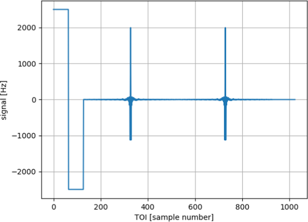
Figure 3. Simulated KISS data block as presented in Fasano et al. (2021). The first, square-shaped samples correspond to the modulation used for the three-point calibration, which is described in depth in Section 2 of Fasano et al. (2021). Then, we observe the forward (left/first) and backward (right/second) interferograms.
Download figure:
Standard image High-resolution image3.3. Observation Mode
One of the objectives of KISS was to prove that atmospheric contamination can be reduced in real time. For this, as discussed above, during astrophysical observations, we decided to set the second input as the constant signal along the focal plane. Assuming that the sky signal is given by the combination of a compact (with respect to the FoV) astrophysical source and the atmospheric emission, we can write

where Bν is the beam pattern and Ω is the observed position on the sky. Ssource(ν) represents the spectrum of the source. Batm(ν) is the averaged atmospheric background signal and δ Batm(ν) atmospheric spatial fluctuations across the FoV. Notice that in these equations we did not account for the displacement of the source during the time of observation of a block.
4. Continuum Analysis and Calibration
4.1. Continuum Signal Reconstruction and Mapmaking
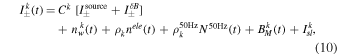
Following the discussion in Section 3, the continuum signal for the kth KID as a function of time can be expressed to first-order approximation as
where Ck is a calibration factor per KID accounting both for response variations between detectors and for a global calibration factor. nk (t) is the detector noise contribution, and nelec(t) represents the detector correlated electronic noise. We assume the atmospheric and electronic correlated noise between detectors with scaling coefficients per KID of Aatm k and Aelec k , respectively. Thus, to correct for the atmospheric and electronic noise, we subtract a baseline and perform a standard decorrelation analysis. We construct a common mode template of the KID signals per array (or per electronic box) and per subscan (regions with constant azimuth or elevation within the scan). In practice, we find that the common signal is dominated by an electronic noise component induced by 50 Hz pickup. With a linear regression analysis, we compute the contribution of this common signal to the data of each KID and subtract it, as well as a constant value per subscan. These corrections are similar to those also applied for spectral data, as further explained in Section 5. The corrected data are then projected into sky maps. In the case of very bright sources (such as the Moon), a simple median baseline per subscan is subtracted.
4.2. Focal Plane Geometry Reconstruction
As is later discussed in Section 4.4, we found the response of the instrument to be severely lower than expected from laboratory measurements (a factor of 30–40 worse). This is expected to be due to the anomalous optical coupling between the QUIJOTE telescope and the KISS camera. This low response implies that even the brightest planets (Jupiter and Venus) are too faint to derive a reliable focal plane geometry (i.e., none of the two are directly visible from individual detector maps).
15
Thus, we used Moon observations to derive the position of each KID in the focal plane and their relative response. We performed a large number of raster scans of the Moon and selected the best ones in terms of weather conditions and instrumental behavior. For each scan, we produced photometric maps per detector and fit the Moon signal on those to both a 2D Gaussian beam and a model of the Moon signal (mainly an uniform disk of  diameter) convolved by the expected beam. Overall, we obtained similar results, but those related to the 2D Gaussian fit proved to be more robust in terms of KID position. The recovered KID positions in the focal plane for the whole set of scans are shown in Figure 4 for arrays A and B. The average from the best scans was used to obtain the final geometry of the focal plane. The results are consistent with the laboratory measurements presented in Appendix B.
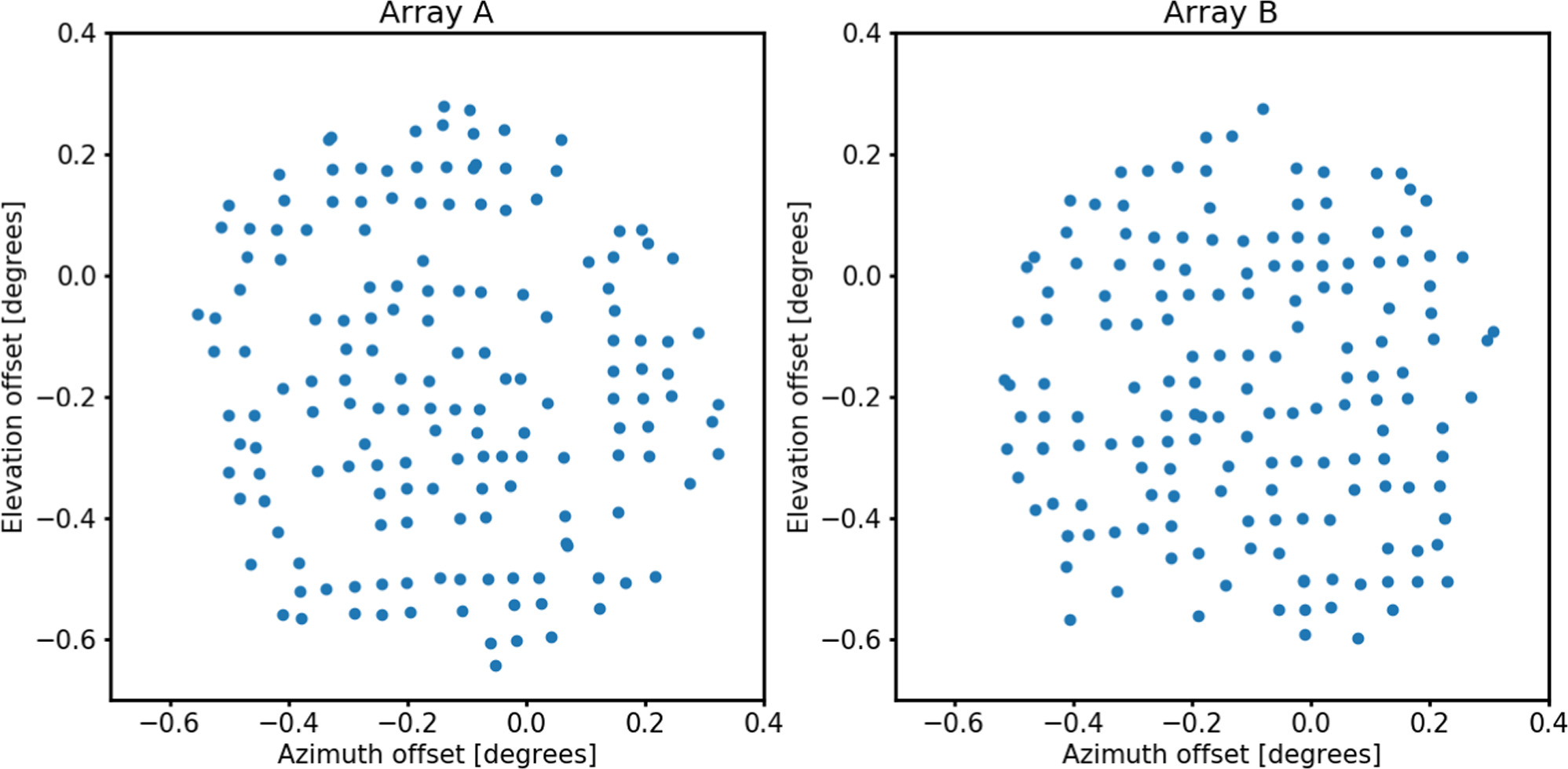
Figure 4. On-sky focal plane geometry. KID offset position for array A (left) and B (right) as computed from the median of available beam map scans on the Moon. The extended nature of the Moon, together with the joint analysis of scans taken at different elevations, explains the variable spacing between detectors (as opposed to the regular spacing obtained from laboratory measurements in Figure 12). We observe some empty regions in the focal plane corresponding to KIDs that were not selected for the final analysis.
Download figure:
Standard image High-resolution image4.3. Focus Optimization
An accurate characterization of the focal distance of the instrument is required in order to prevent a significant degradation of the properties of its beam. This would be translated into an increase of its ellipticity and FWHM; both would also imply a loss of the integrated flux (assuming in both cases a resolved source). The position of the focal plane with respect to the optical system can be changed in order to calibrate the optimal focus position (or focal distance). This corresponds to 20 mm with respect to the dedicated camera mount on the telescope. In the top plots of Figure 5, we show maps of Jupiter performed at different focus positions. By fitting the Jupiter signal to a 2D circular Gaussian, we obtain the FHWM and amplitude as shown in the bottom panels. The lowest FWHM values and flux losses are achieved for focal distances, with respect the telescope mount, between 16 and 18 mm, respectively. The results presented in this paper were obtained for a distance of 18 mm with respect to the telescope mount. We measured little to no variation in the beam properties with elevation, and the KISS sensitivity degradation due to the suboptimal QUIJOTE/KISS coupling (as presented below) did not degrade the beam properties. Therefore, we used an average focus offset along all observable elevation angles (30°–90°).
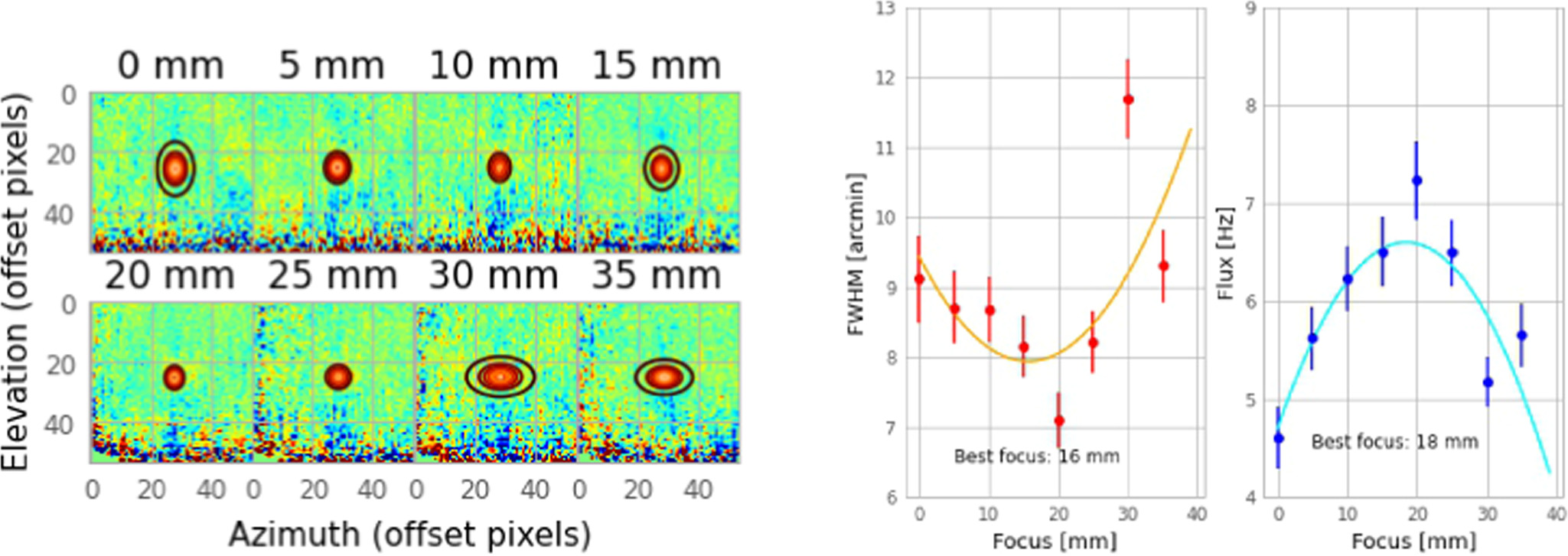
Figure 5. Focus. Top: Jupiter maps at 150 GHz obtained from the combination of all detectors for different focus distances. Low (high) values return prolate (oblate) morphologies. Bottom: changes in the maximum FWHM of the disks and the integrated flux with variable focus distance.
Download figure:
Standard image High-resolution image4.3.1. Absolute Continuum Calibration
We used Jupiter as the main KISS continuum calibrator. The Jupiter brightness temperature used here is derived from the ESA 1 model (Planck Collaboration et al. 2017) and is equal to 170 ± 8 K at 150 GHz. All Jupiter scans showing a reduced level of noise residuals have been considered, returning consistent values independent from the atmospheric opacity or the elevation and between the A and B KID arrays. In Figure 6, we show the distribution of the calibration factors obtained for all the scans considered. This distribution is consistent with a Gaussian distribution with a mean value of 35.7 ± 2.6 Hz K−1. Absolute uncertainties on the model of the brightness temperature are expected to be of the order of 5% and are accounted for in the following.
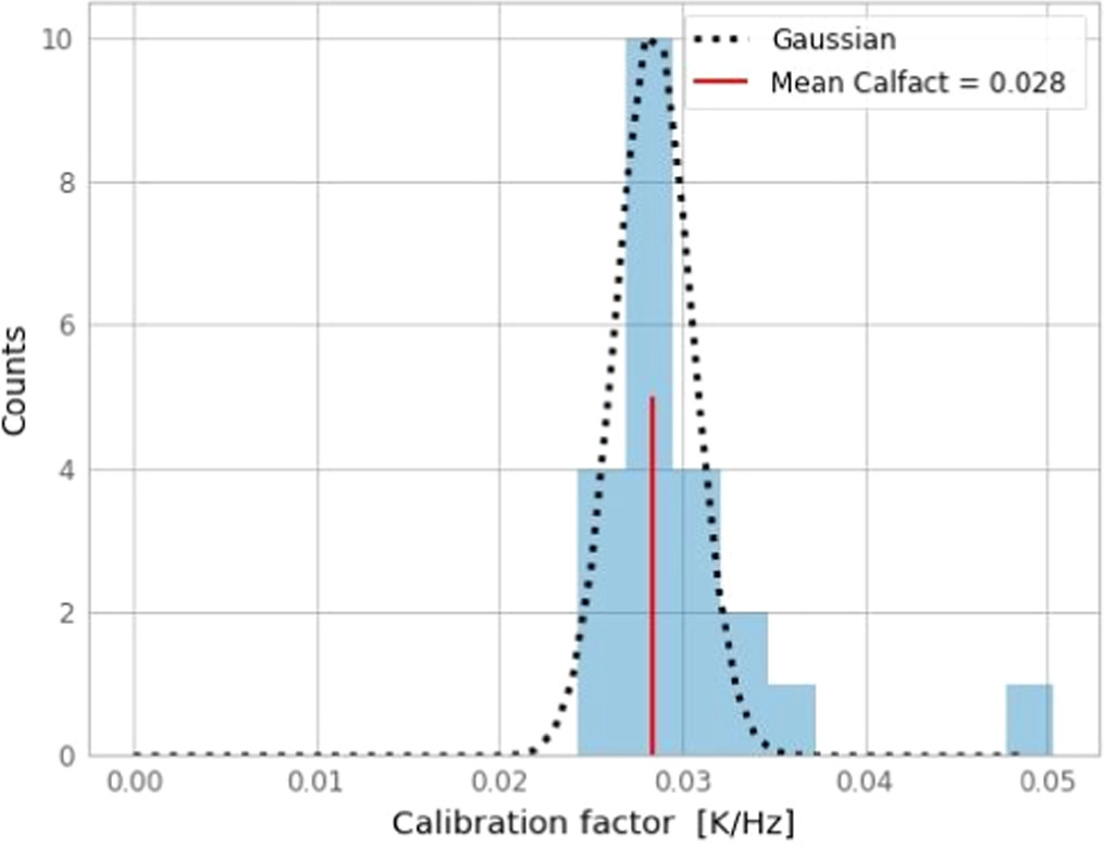
Figure 6. Distribution of the joint continuum calibration factors for the A and B KID arrays obtained from the selected Jupiter measurements. The mean value and uncertainties presented in the figure are considered for the results presented in this paper.
Download figure:
Standard image High-resolution image4.4. Continuum Sensitivity
To obtain the final noise level in the KISS observations, we have directly computed the white-noise level in the Time Ordered Information (TOIs) and neglected the contribution from correlated atmospheric and electronic noise, which could lead to residual noise in the maps. We obtain a white-noise level ranging between 1.5 and 2.5 Hz s1/2. This value is compatible with the detector noise measured in the laboratory and indicates that the detector behaves as expected. When accounting for the calibration value from Section 4.3.1, this white-noise level translates to 60–80 mK s1/2 and an NEFD = 140–180 Jy s1/2, after multiplying by the KISS solid angle. This is a large value compared to those from NIKA2 (9 mJy s1/2; Perotto et al. 2020) or CONCERTO (∼70 mJy s1/2; Hu et al. 2024). This low overall response from on-telescope data is expected to be due to the suboptimal coupling between the instrument and the telescope. Indeed, it was not observed during the laboratory characterization of the former, when calibration factors of ∼1000 Hz K−1 were obtained. In Section 6.1.1, we discuss how the ratio between these laboratory factors and the ones obtained from on-telescope data is around 30. When correcting for this degradation factor, together with the larger beam of KISS, the results are consistent with the previously mentioned NIKA and CONCERTO estimates.
5. Spectroscopic Analysis and Calibration
5.1. Data Model
5.1.1. Sky Signal
Starting from the signal model discussed in Section 3, we now describe the general data model of the measured interferograms for each detector. Based on Equation (6), we can write
where the ± subscript reflects the sign difference between KIDs in the A (in-transmission) and B (in-reflection) arrays.
5.1.2. Detector and Electronic Noise
Laboratory dark measurements have shown that the KID intrinsic noise can be considered white to first order. Furthermore, the analyses of NIKA and NIKA2 data (Perotto et al. 2020) have shown that the detected Gaussian detector correlated noise is related to the acquisition readout. In the following, the detector and electronic noise components will be noted as

similarly to the components already present in Equation (7). During operations, we identified a rather constant sinusoidal electrical signal that induces an additional noise component in the KISS detectors. As shown in Figure 7, this sinusoidal signal has a typical period of 8–12 samples at 3.816 kHz, and its amplitude is modulated with time. The exact origin of this signal is not known, but it seems to be related to the electrical installation of the telescope and its coupling with the instrument. In the following, we will refer to this signal as the 50 Hz pickup,  , as it seems to be a harmonic of 50 Hz.
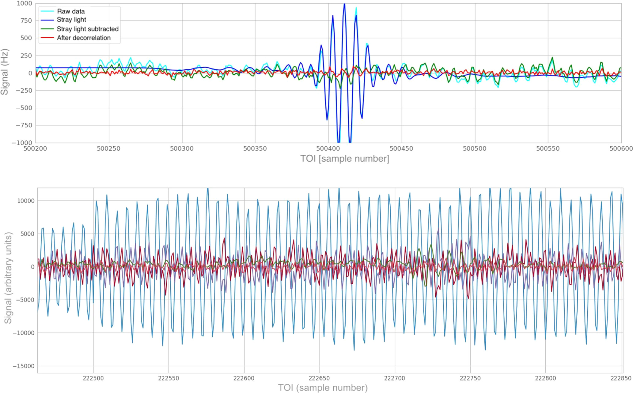
Figure 7. Top: example of KISS data after each of the steps of the data processing. The cyan line represents the raw acquired data, while the dark blue line represents the mean stray-light contribution that effectively dominates the signal. The difference between the two is shown as the green line. The dominant component at this stage of the data processing is the 50 Hz electrical pickup signal. In order to get rid of this signal (and other residual ones), a PCA is performed to estimate the noise behavior. The final decorrelated signal, which will be projected to the maps and used for scientific purposes, is shown in red. Bottom: PCA components associated with the five most significant eigenvalues. These are used as template to correct for the systematic contribution discussed above (the data are assumed to be a linear combination of those templates). This correction is done independently for each KISS scan.
Download figure:
Standard image High-resolution image5.1.3. Parasitic Mirror Signal
We identified a parasitic signal for some of the detectors that can be related to a modulation of the background between forward and backward interferograms. This is expected to be due to stray light entering the optical system when moving the displacement mirror. Therefore, it should be periodic with respect to the mirror position, and we will denote it as  .
.
5.1.4. Stray-light Background
We have found that the KISS interferograms present a constant background signal that seems to be from environment stray light, Ik sl . This signal fully dominates the observed interferograms and needs to be removed prior to the sky projection. The background signal is expected to be consistent with a Rayleigh–Jeans spectrum at room temperature.
5.1.5. Overall Model
After coadding all the components, the interferometric signal measured by a detector k can be written as
where the first two terms account for Equation (8), the former for the difference between the inputs and the latter for the atmosphere fluctuations.
5.1.6. Other Possible Systematic Effects
Other systematic effects can affect the reconstruction of the spectrum for a generic FTS. In the case of KISS, the lack of instrumental response at the telescope prevented us from studying those in detail. We just mention the most important ones here and comment on their mitigation during instrumental design and laboratory testing. An important concern during the design process was to ensure a homogeneous illumination of the focal plane and in particular of off-axis pixels. The shapes of the KISS mirrors and lenses were optimized accordingly, and we slightly underilluminated the telescope. Another important systematic effect comes from the difference in the optical path or misalignment of the two arms of the interferometer. To correct for this, we extensively performed alignment campaigns both during tests in the laboratory and prior to telescope installation. The alignment was considered optimal when maximizing the amplitude of the interferograms for all detectors. We observed no hint of misalignment on the sky data. We have also considered variations in the optical path induced by vibrations either of the mechanical system or of the beam splitter. For the former, as discussed above, we considered a spiral spring and a two-opposite-motors system that made the mechanical vibrations' contribution to the data negligible. Vibrations of the beam splitter can produce inhomogeneous time variations of the optical path across the FoV and lead to differences in the sampling of the OPD (not in accordance with the measurement from the laser monitoring) and the position of the ZPD. For KISS, we only observed time constant variations of the ZPD position across the FoV as discussed above. Finally, we have observed variations between the OPD sampling for the forward and backward interferograms, but those can be corrected using the laser monitoring.
5.2. Spectroscopic Signal Reconstruction and Mapmaking
As shown in Equation (3), after the three-point calibration has been performed, we construct independent arrays containing the forward and backward interferograms for each detector and each block. For the sake of clarity, we express the different contributions to the raw interferograms described above in terms of detector, block, and block position indices (ik, ib, ip). We notice that the observation time is proportional to t = (ib ∗ Nspb + ip) × (1/fsampling) + t0, and so we can write
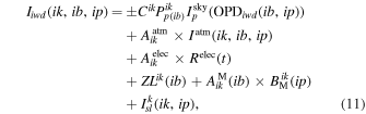
where iwd defines either the forward or backward raw interferograms. We define the offset path difference as a function of time as OPD(ib, ip) = ZPD(ib, ip) − 2Δd(t)/c. The atmospheric residual signal is assumed to be common between neighbor detectors to a given scaling factor. The electronic noise is assumed to be common for all detectors with a single scaling factor per scan. The parasitic mirror signal is modeled per block and per detector as a constant offset, ZL, and a scaled function, BM. Finally, we assume the stray-light background signal to be constant with time.
5.2.1. Preprocessing
In order to isolate the real astrophysical signal,  , from the rest of the components, several processing steps are applied separately for forward and backward interferograms.
- 1.A linear fit is subtracted from each interferogram within each block in order to account for the mirror parasitic contribution.
- 2.The ZPD is computed from the mean interferogram for each detector.
- 3.The mean interferogram per detector and per scan is subtracted from all (forward or backward) interferograms. In this way, the stray-light contribution is subtracted in OPD space. Strong sources are masked before computing the mean interferogram.
5.2.2. Correlated Noise Removal
The atmospheric and other correlated noise components can be subtracted by applying a principal component analysis (PCA) decorrelation algorithm. This analysis is run by comparing the data from all the different detectors (ik) in a given array and deriving common PCA templates accounting for both detector and electronic noise components. In practice, we consider the first five PCA components, which seem to account for most of the unwanted components in the data.
We show in Figure 7 an example of the full processing on the KISS interferograms, taken from a Jupiter scan. We show the forward raw interferograms for one detector and block of data (cyan) after correction of the mirror parasitic signal. In blue, we show the mean interferogram, which mainly accounts for the stray-light background signal. In green, we show the residual atmospheric and electronic noise, which show an oscillatory behavior. The PCA decorrelated interferogram is shown in red. We observe that there are various orders of magnitude in amplitude with respect to the raw data.
5.2.3. Projection of Interferograms on the Sky and Spectral Inversion
The processed interferograms for all detectors in one array are jointly projected into the sky in OPD space using a simple coaddition method to obtain interferometric cubes 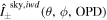 for the forward and backward interferograms. A total of 801 bins in OPD were selected to ensure a good representation of the interferograms, in particular in the region of the maximum. This also allows us to fully cover the frequency range of interest for KISS.
Combining the forward and backward interferogram cubes and taking the Fourier transform, we can obtain an estimate of the spectrum of the sky,
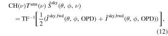
where C defines the overall calibration coefficient after the KID combination.
5.3. Calibration
As for the continuum case, the spectroscopic calibration was made using Jupiter scans and assuming the Jupiter SED model from Section 4.3.1. As we have only considered compact sources, we have decided not to rely on bandpass reconstruction, and as such, we define a combined spectral calibration coefficient, C(ν) = CH(ν). These coefficients per frequency are computed from the flux of Jupiter at each frequency as measured on the spectral cubes defined above. In practice, we construct spectral cubes for the two arrays for each of the scans of Jupiter. We compute the flux of Jupiter at each frequency by fitting the frequency map to a 2D Gaussian. The obtained flux is corrected for atmospheric transmission using an Atmospheric Transmission Model model (Pardo 2019) and the on-site measurements (Castro-Almazán et al. 2016) of precipitable water vapor (PWV). These PWV measurements are taken by a GPS antenna located at ∼1 km of the telescope, which obtains four rapid measurements and one precise measurement per hour. Finally, after comparing the measured flux with the expected Jupiter SED, we obtain the spectral calibration coefficients. 16
These coefficients as well as the best-fit FWHM are shown in Figure 8. In the top plots, we show both individual scans (gray lines) as well as mean (blue) and median (red) spectral calibration coefficients. In the bottom plots, we show the measured FWHM as a function of frequency. We observe that the FWHM values from spectroscopic data are consistent with the expected behavior in frequency as derived from continuum measurements (blue line) from Section 6. The highest-frequency point is already too close to the 180 GHz water vapor line, which implies a much larger and poorly defined calibration factor at that frequency range. We also see great variations in the beam size across scans. Both issues are especially severe for array B, as can be seen in the two panels on the right. The latter issue suggests that this point is not only noisier because of the water vapor line but might also be biased.
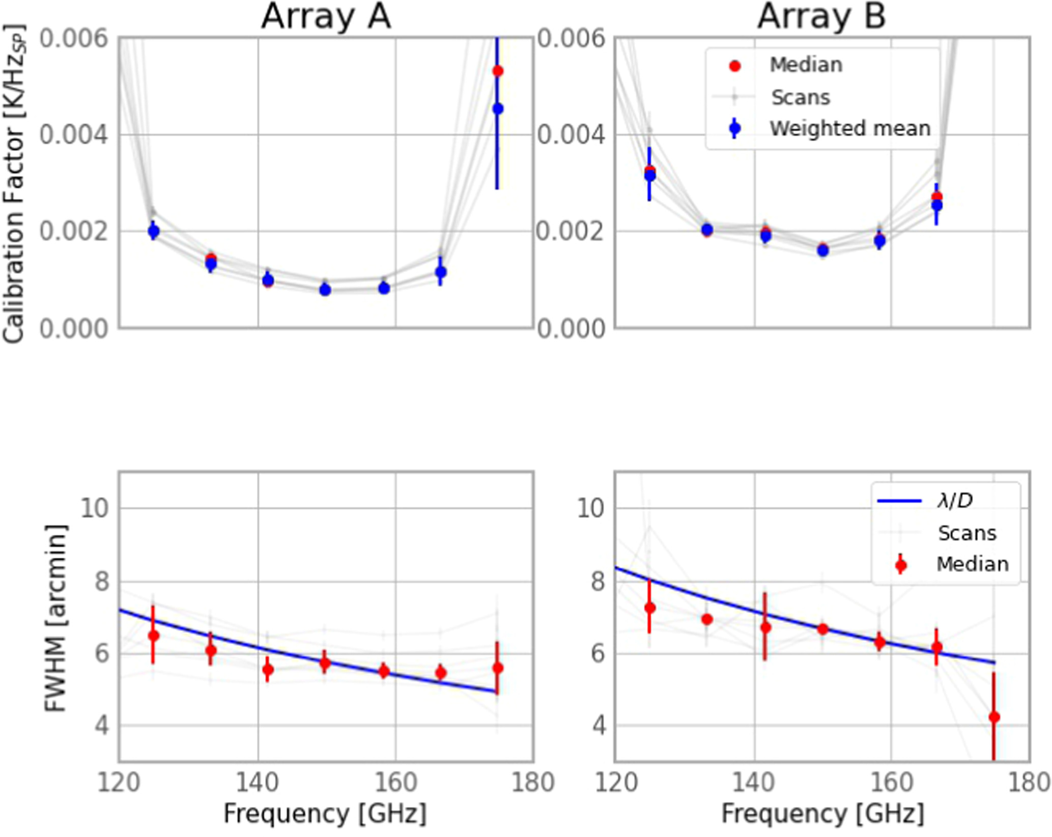
Figure 8. Spectroscopic calibration coefficient (top) and beam FWHM (bottom) per frequency as derived from Jupiter observations for the A (left) and B (right) arrays. The calibration factors are computed as in Section 4.3.1, through aperture photometry at each of the frequencies considered.
Download figure:
Standard image High-resolution image6. Continuum and Spectral Maps of Selected Astrophysical Targets
We have performed sourced-centered azimuth-elevation raster scans to map the sky sources. In practice, we perform two consecutive subscans and then repoint the telescope to follow the source motion. The main properties of the scans are the center azimuth and elevation positions, the map size in the two axes, the step between two consecutive subscans, and the scanning velocity. These observations are prepared and controlled using a new graphical user interface (GUI) customized for KISS. This GUI has been optimized to be used jointly with the control software of the QUIJOTE telescopes, based on Twincat (Gómez-Reñasco et al. 2012). One of the main tasks of this GUI is to send the telescope status and position to the KISS acquisition system in order to control the tuning procedure of the KIDs. A complete description of this tuning procedure is presented in Bounmy et al. (2022).
6.1. Moon Observations
We took a total of 284 raster scans of the Moon during the KISS observation run. Each of them lasted for 10 minutes, accounting for almost 50 hr at the end. The sizes of the maps varied greatly, with most of them being between  and
and  . Most of these scans show issues, especially before 2019 November 22, when the first complete pointing model version was applied.
17
After discarding data showing issues, we end up with a final set of 52 Moon rasters. These Moon rasters were taken on five different dates between 2019 November 22 and 2020 November 9.
. Most of these scans show issues, especially before 2019 November 22, when the first complete pointing model version was applied.
17
After discarding data showing issues, we end up with a final set of 52 Moon rasters. These Moon rasters were taken on five different dates between 2019 November 22 and 2020 November 9.
6.1.1. Moon Photometry
In Figure 9, an example photometry map from one of the Moon rasters is shown. This scan corresponds to the brightest Moon observation within our sample, while the Moon was in its full phase. Because of that, the Moon is evenly illuminated by the Sun, and its brightness can be assumed as uniform within its disk. That implies that, when studying the angular size of the Moon emission, a Gaussian fit in both directions is enough when the Moon is in its full phase. Thus, we find the FWHM of the best Gaussian fit to be consistent with the expected Moon angular size (30′). When using the FWHM values obtained for the two axes (a, b), we find an ellipticity value of just e = 1 − b/a = 0.024.
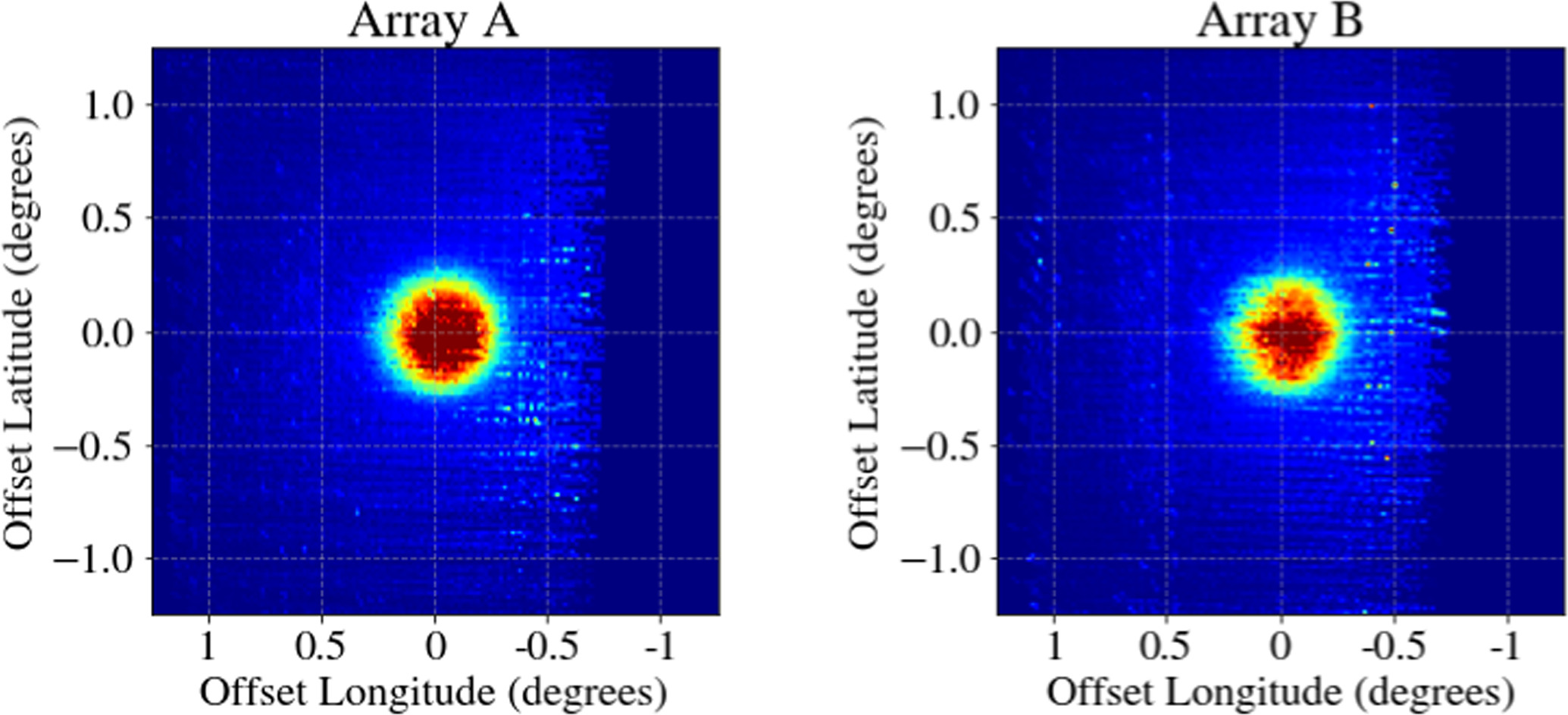
Figure 9. Continuum maps (left/right: A/B arrays) for a Moon observation taken on 2019 December 9. This is the brightest observation from our sample. We measured the offset on the obtained Moon image with respect to its expected position in order to look for residual deviations in the pointing model. These are only found at the subarcminute level, proving that the pointing model (which was obtained at the TOI level; see Appendix C) works well.
Download figure:
Standard image High-resolution imageThe Moon flux is estimated using aperture photometry. The median signal within a ring with radii  and 40′, which accounts for the background signal, is subtracted from the mean signal within a disk of radius 20′. The standard deviation of the signal within the former region is used to estimate the uncertainty of the measurement. We then studied these flux values as a function of time and compared them to the models for the lunar phase from Krotikov & Pelyushenko (1987, hereafter KP87) and Hafez et al. (2014, hereafter H14). For this, we assumed an effective frequency of 150 GHz for the Moon observations, close to the central frequency of KISS:

where ω is the angular frequency of the Moon cycle (360◦/29.35 days = 1226 days−1). t is the elapsed time since a reference new Moon, which we selected as 05:31:31.2 from 2019 December 12. The parameters defining the KP87 model are i ∈ (1, 2, 3, 4), Ti
∈ (107, 19, 15, 7) K, and ϕi
∈ (14, 26, 20, 34)°. The model is scaled by a constant value to obtain the calibration factor between the brightness temperature and the signal in frequency units. An offset constant value is also taken into account. In Figure 10, we show the fitted data and best-fit models. The two calibration factors for KID array A are 27.5 ± 6.3 Hz K−1 for the KP87 model and 33.8 ± 6.6 Hz K−1 for the H14 model, the two being consistent within 1σ. The same factors for KID array B are 24.1 ± 4.18 Hz K−1 and 29.4 ± 4.4 Hz K−1, respectively, again consistent within 1σ. Considering that the laboratory measurements of the gain returned values in the 1000 Hz K−1 range, the deficit is around a factor of 30–40.
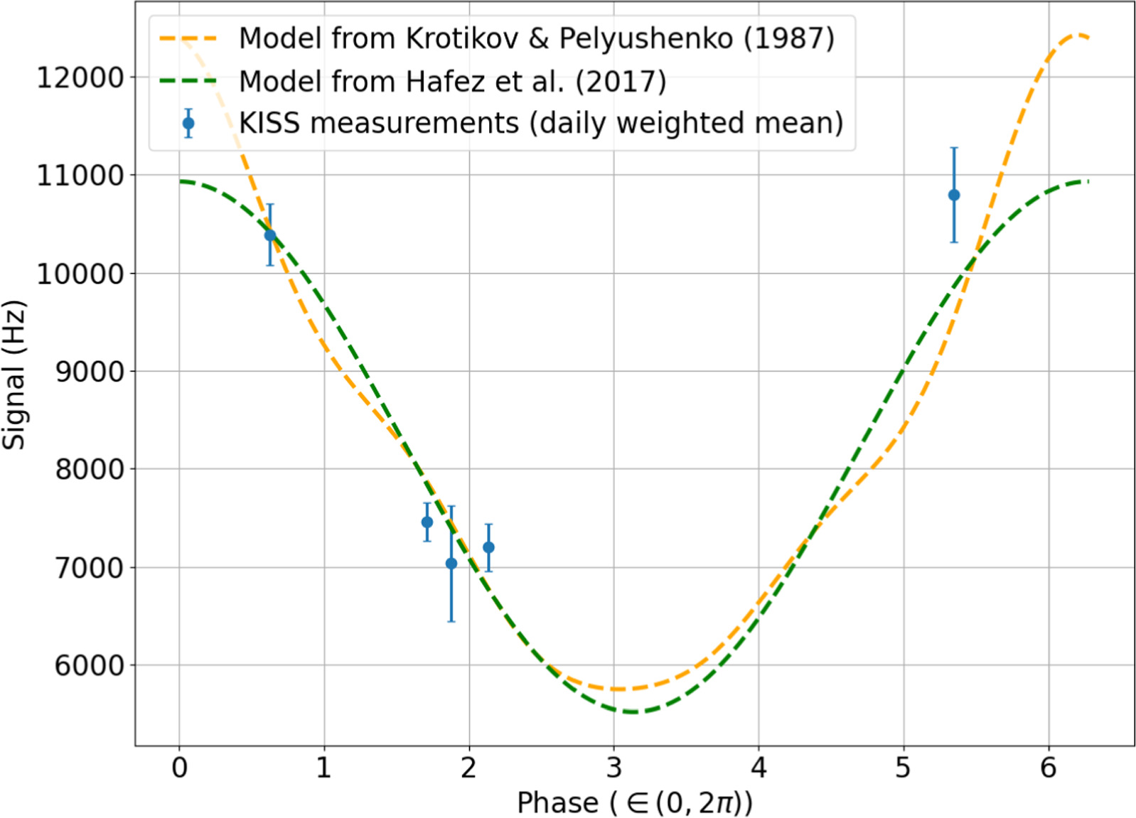
Figure 10. Comparison between the brightness temperature obtained for the Moon from the data and the models from KP87 and H14. The models have been scaled from brightness temperature to frequency units by a constant factor plus an offset value. This has been computed as the one minimizing the quadratic sum of the differences with respect to the data along the full phase. The five different observation dates account for reduced coverage of the phase. Data for KID array A.
Download figure:
Standard image High-resolution imageThese values are roughly consistent with the one from Jupiter obtained in Section 4.3.1 (Figure 6), 35.7 ± 2.6 Hz K−1, the worst of them being 2.4σ away. The agreement is better with array A than array B. The lower gain could be pointing to a deficit of signal in the KID response because of the extended nature of the Moon compared to that from Jupiter or to nonlinearities in the instrument response when under large signals. It can also be due to an oversubtraction of the signal when calculating the mean over the full FoV to estimate the baseline level because of the larger Moon size. These results confirm the issue with the optical coupling between the QUIJOTE telescope and the KISS instrument.
KISS spectral maps and data from the Moon were already presented in Fasano et al. (2020b). In that case, a notch filter was included to discard the emission from the 180 GHz water vapor line while being able to observe from 200 to 300 GHz. The observations described in this work, on the other hand, completely filtered out all emission above 180 GHz. Below this frequency, both spectral analyses are consistent.
6.2. Venus Spectra
We obtained 40 Venus scans after the final pointing model was in place. These account for almost 7 hr of observations, each scan being around 10 minutes long and covering a  region. Continuum results using KISS for Venus were already published in Fasano et al. (2021) and are presented here for the record in Figure 11 in bright red. This is compared with several ancillary observations at radio frequencies between 1 and 100 GHz, showing a consistent behavior. We also show for comparison (as in Fasano et al. 2021) the Bellotti & Steffes (2015) model (blue solid and dashed lines) and simple best-fit power law (cyan data). Notice that we also included in the figure data from recent measurements with the QUIJOTE telescope in the 10–19 GHz range (Rubiño-Martín et al. 2023).
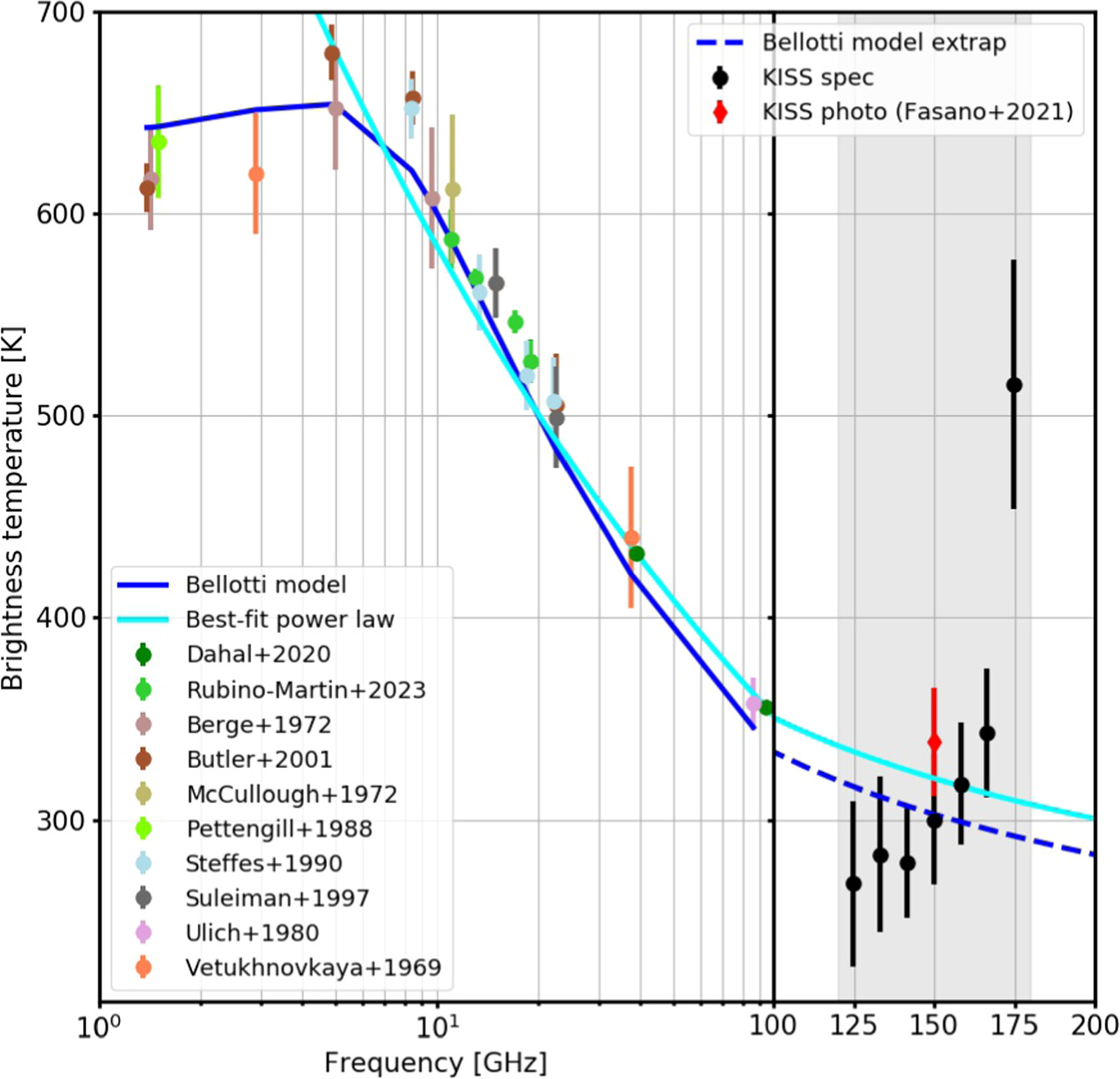
Figure 11. Comparison between the Venus continuum (light red dot) and the spectrum (black dots) obtained from KISS with ancillary data and models. At the edges of the KISS band, we expect the systematic uncertainties to be large, as the transmission is low. This explains why the KISS highest-frequency point is significantly above the model. A detailed description of the former is given in Fasano et al. (2021). We also include recent results from the QUIJOTE experiment in the 10–20 GHz frequency range (Rubiño-Martín et al. 2023).
Download figure:
Standard image High-resolution imageWe have obtained the spectrum from the same Venus data using the approach described in Section 5. The obtained spectral density is shown as black dots in the figure. Uncertainties were computed from the dispersion between scans and also include the absolute calibration uncertainties presented in Section 5.3. The uncertainties are dominated by the latter and in particular at the edges of the KISS band. This is particularly obvious at high frequency, for which systematic uncertainties dominate the signal. Overall, our measurements are consistent with the two aforementioned models proposed at the 95% confidence limit.
7. Conclusions and Perspectives
This is the last of several papers describing the performance of the KISS instrument (Fasano et al. 2020a, 2020b, 2021). We have shown that the KIDs and interferometers (and, more specifically, an MPI) can be used together to provide simultaneous photometric and spectral measurements of astrophysical targets in the millimeter range (between 100 and 180 GHz). The beam properties of the instrument matched those from its design phase, achieving FWHM values of 7′–8′ at 150 GHz over the large KISS FoV (1°). The recovered focal plane geometry also followed the one measured at the laboratory, with ∼80% of the KIDs working normally.
The main issue that we encountered during the observation phase of the instrument was a deficit in its response with respect to the one expected. This deficit is of the order of a factor of 30 and is expected to be due to a miscoupling between the instrument and the telescope. It is possible that despite the fact that the QUIJOTE telescope was designed up to millimeter wavelength, aging and environmental conditions have degraded its performance. Furthermore, we notice, first, that such an issue was not observed during KISS laboratory testing, and second, that no problem was found during the CONCERTO commissioning phase (Hu et al. 2024). As such, we are confident that the deficit of response is not related to the instrumental design of KISS.
This degraded response prevented KISS from fulfilling its second main objective: to provide measurements of the SZe from large GCs. However, it did not prevent KISS from being a reliable test bench for CONCERTO (CONCERTO Collaboration et al. 2020). This was particularly the case for the optical configuration and the readout, the raw calibration methodology, and the development of the data analysis pipeline.
Jupiter and Venus were observed with a sufficient signal-to-noise ratio to measure their SED. Moon observations were also used to show the slight differences encountered when observing an extended source. The phase of the Moon is well recovered from our data, showing that the calibration factor did not vary greatly during our observing run. Finally, our results show the promising prospects of the combination of KIDs with interferometers to provide simultaneous photometric and spectral measurements.
Acknowledgments
We thank the staff of the Teide Observatory for invaluable assistance in the commissioning and operation of QUIJOTE. The QUIJOTE experiment is being developed by the Instituto de Astrofisica de Canarias (IAC), the Instituto de Fisica de Cantabria (IFCA), and the Universities of Cantabria, Manchester, and Cambridge. Partial financial support was provided by the Spanish Ministry of Science and Innovation under the projects AYA2017-84185-P and PID2020-120514GB-I00. We thank Angelo Mattei of the Mechanical Workshop Service of the INFN Rome 1 Section for manufacturing the HDPE lenses. M.F.T. acknowledges funding from the French Programme d’investissements d’avenir through the Enigmass Labex and support from the Agencia Estatal de Investigación (AEI) of the Ministerio de Ciencia, Innovación y Universidades (MCIU) and the European Social Fund (ESF) under a grant with reference PRE-C-2018-0067. This project has been partially supported by the European Research Council (ERC) under the European Union's Horizon 2020 research and innovation program (grant agreement No. 788212) and by the LabEx FOCUS ANR-11-LABX-0013.
Software: astropy (Astropy Collaboration et al. 2013, 2018, 2022), matplotlib (Hunter 2007), numpy (Harris et al. 2020), scipy (Virtanen et al. 2020).
Appendix A: Interferometric Equation Derivation
Assuming a monochromatic input signal, focusing on S1, and following the notations of Figure 2, we can write the electric field for each of the previously described steps:
Reflections on the M1 and M2 mirrors lead to  and
and  . For the combined beam, we have
  ; therefore,

After the output polarizer, P2, the observed intensity in the KID arrays can be written as  and
and  , where
  and
and  are unitary vectors along the x- and y-axes. Therefore, we can write
where 2Δd(t) is the OPD between the two roof mirrors at time t.
Appendix B: Laboratory Measurements
During laboratory tests, we were able to reconstruct the position of the KIDs in the focal plane using a background sky simulator coupled to a fake planet. The sky simulator, consisting of cold head coupled to a pulse tube, produces a nearly homogeneous sky temperature. The fake planet, made of a metal ball attached to a metal arm by a kevlar wire, can be displaced vertically and horizontally to mimic raster scans, which were used to derive the focal plane geometry. For each scan, the raw data were projected into maps per KID, and these were fitted to a 2D Gaussian to derive the KID position in the focal plane, the beam FWHM and ellipticity, and the relative KID response. Figure 12 shows the reconstructed position of the KIDs in the focal plane for array A (left) and B (left). The 1° FoV is fully sampled, with better coverage in the center part and in the outer region. In Figure 13, we present the main measured properties of the KIDs in terms of beam FWHM and ellipticity and amplitude. We observe that the KIDs have similar properties with nominal behavior, about 6–7 mm FWHM. The small excess of ellipticity is mainly due to signal from the wire.
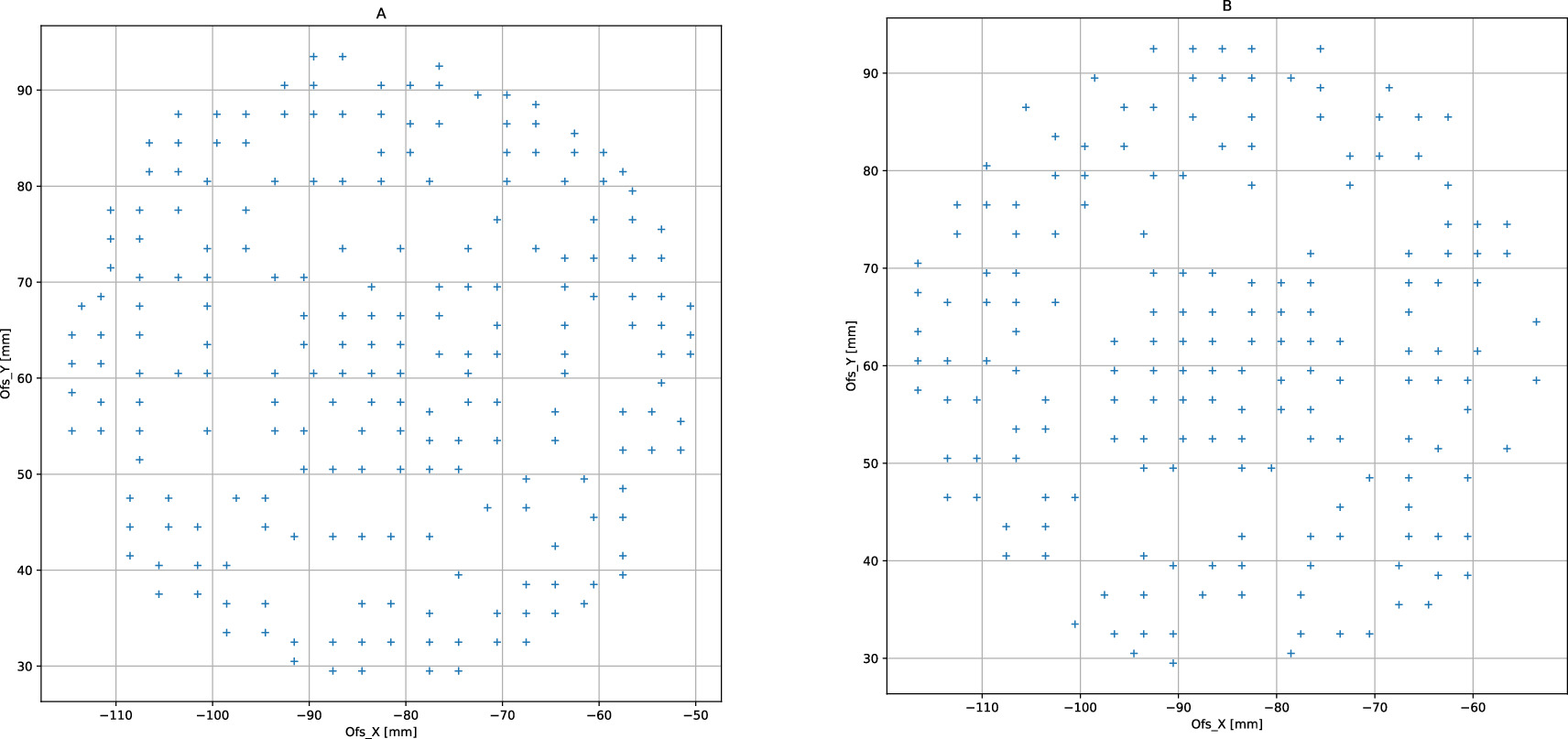
Figure 12. Geometry of the focal plane from laboratory measurements. KID offset position for arrays A (left) and B (right).
Download figure:
Standard image High-resolution image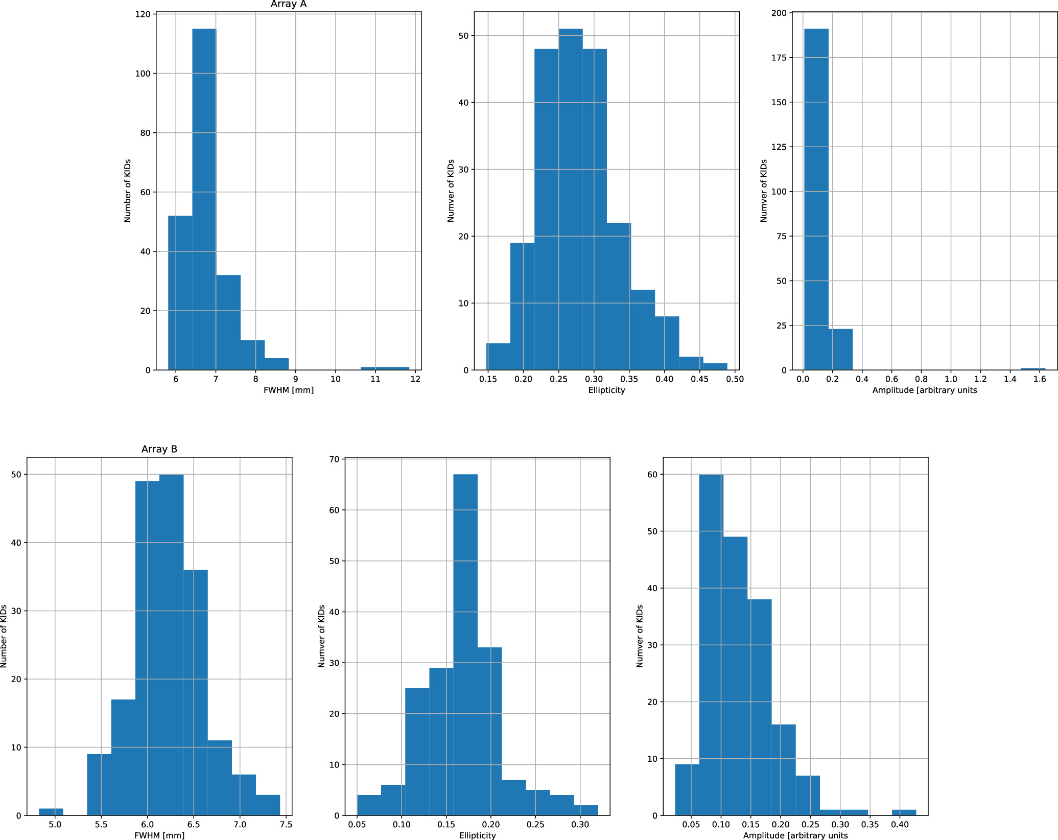
Figure 13. Measurements of KID FWHM, ellipticity, and response/amplitude (from left to right) obtained from laboratory measurements. Results for arrays A (top) and B (bottom).
Download figure:
Standard image High-resolution imageAppendix C: Pointing Model
The pointing was reconstructed using measurements of the Moon, Jupiter, and Venus. A first pointing model was obtained from Moon observations only (Figure 14), and then it was refined using the observations of the planets. The final pointing model consists of seven parameters (Figure 15). The description of these parameters can be found in Wallace (2008). The pointing model parameters were derived from the time-ordered data of detector KA005, which is at the center of array A. The astrophysical signal was modeled assuming a 2D Gaussian beam with FWHM equal to 30′ for the Moon and 7′ for the planets.
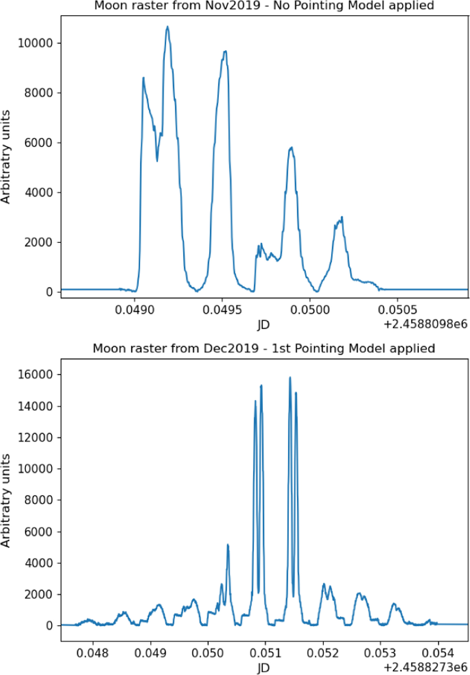
Figure 14. Top (bottom): example of a Moon raster before (after) applying the first version of the pointing model. This version only used Moon data and fixed the azimuth and elevation offsets between the sky and the telescope encoder. The improvement is already noticeable, as the expected double-peaked behavior emerges after applying this preliminary version of the pointing model. The steep angular features close to the peaks, typical of an imperfect pointing model, also lose prominence after applying this first version of the pointing model.
Download figure:
Standard image High-resolution image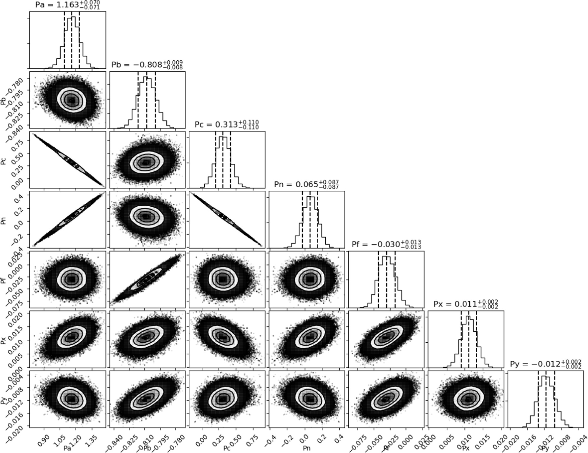
Figure 15. Corner plot showing the posteriors for the final values of the pointing model using data from Moon, Jupiter, and Venus observations. There are degeneracies between the azimuth-related (Pa , Pc , Pn ) and elevation-related (Pf , Pb ) parameters due to the lack of calibrators for every azimuth-elevation position. Units are in degrees.
Download figure:
Standard image High-resolution imageFootnotes
- 12
Located at 2400 m of altitude in Tenerife, Spain.
- 13
Corresponding to two interferograms per block of 1024 samples with a sampling rate of 3.816 kHz.
- 14
This means that, in reality, fewer than four blocks (3.816) are registered each second.
- 15
- 16
In principle, the ATM model could be used together with a skydip observation in order to provide an independent calibration estimate. However, we have observed different near (atmosphere) and far (targets) field responses. Therefore, we decided to calibrate using only the planets.
- 17
The pointing model is described in depth in Appendix C.