ABSTRACT
We present the results of an intensive multiwavelength campaign on nova LMC 2012. This nova evolved very rapidly in all observed wavelengths. The time to fall two magnitudes in the V band was only 2 days. In X-rays the super soft phase began 13 ± 5 days after discovery and ended around day 50 after discovery. During the super soft phase, the Swift/XRT and Chandra spectra were consistent with the underlying white dwarf (WD) being very hot, ∼1 MK, and luminous, ∼1038 erg s−1. The UV, optical, and near-IR photometry showed a periodic variation after the initial and rapid fading had ended. Timing analysis revealed a consistent 19.24 ± 0.03 hr period in all UV, optical, and near-IR bands with amplitudes of ∼0.3 mag which we associate with the orbital period of the central binary. No periods were detected in the corresponding X-ray data sets. A moderately high inclination system, i = 60 ± 10 , was inferred from the early optical emission lines. The HST/STIS UV spectra were highly unusual with only the N v (1240 Å) line present and superposed on a blue continuum. The lack of emission lines and the observed UV and optical continua from four epochs can be fit with a low mass ejection event, ∼10−6
  , from a hot and massive WD near the Chandrasekhar limit. The WD, in turn, significantly illuminated its subgiant companion which provided the bulk of the observed UV/optical continuum emission at the later dates. The inferred extreme WD characteristics and low mass ejection event favor nova LMC 2012 being a recurrent nova of the U Sco subclass.
1. INTRODUCTION
Nova explosions occur in binary systems when a white dwarf (WD) accretes a sufficient amount of mass lost from its companion, either from Roche lobe overflow in short period systems or a wind in long period systems, to initiate thermonuclear reactions. Core material in the WD is mixed into the accreted layers and the envelope is violently ejected when the pressure at the degenerate WD-accretion interface becomes high enough to trigger a thermonuclear runaway (TNR). Novae thus expel a mixture of accreted gas, material from the underlying WD, and products of nucleosynthesis from the TNR. The amount of mass accreted and subsequently ejected, and the energetics of the outburst, depend on the WD mass and composition plus the accretion rate.
While there have been many multiwavelength studies of Galactic (Schwarz et al. 2011) and M31 novae (Henze et al. 2014; Shafter et al. 2011), there are rather few for those in the Magellanic Clouds. Novae in the clouds have the advantage of coming from a more homogeneous population than in the Galaxy and are effectively at the same distance and low extinction. Since the LMC is significantly closer than M31, its novae can be followed well into their nebular phases. This is currently impossible for M31 novae since they generally fade below the optical/near-IR (NIR) background after a decline of only a few magnitudes.
Nova LMC 2012 (TCP J04550000-7027150; LMCN 2012-03a) was discovered on March 26.397 UT (MJD 56012.897) at a visual magnitude of 10.7 (Seach et al. 2012). The upper limit on the visual magnitude was 12.5 mag 12 days prior to the Seach discovery. The discovery date is taken as day zero and the shorthand “Dn,” where “n” is the number of days after day zero, is used for all the following observations. Figure 1 shows the V band light curve. The early visual and unfiltered estimates given in Seach et al. (2012) are also included for completeness. The last visual estimate was about 0.5 mag brighter than the V band observation taken at the same time. This is typical of visual magnitudes since they are more sensitive to Hα emission, due to the red sensitivity of the human eye. With this correction, we estimate that LMC 2012 likely reached V maximum on D0.3 at <11 mag. The time to decline two and three magnitudes ( ) using only the observed V band photometry was 2 and 4.5 days, respectively. These are upper limits since there was no V band photometry prior to D0.6 and the decline is faster just after maximum. These optical declines are similar to V838 Her (Vanlandingham et al. 1996) and V4160 Sgr (Schwarz et al. 2007) which makes LMC 2012 one of the photometrically fastest novae ever observed.
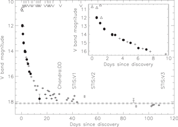
Figure 1. SMARTS (pluses) and AAVSO (filled circles) V-band light curve. The earliest visual estimates from Seach et al. (2012) are shown as triangles. The times of the three HST/STIS observations, a Chandra DDT observation, and SMARTS spectroscopy (downward arrows at top) are also labeled. The dotted line is the V-band magnitude of the nearby field star (Zaritsky et al. 2004) with the dashed lines showing its uncertainty. The inset shows the early decline in greater detail.
Download figure:
Standard image High-resolution imagePrieto (2012) obtained an optical spectrum on D0.4. The spectrum had strong, broad emission lines with P-Cygni profiles. The absorption troughs of the P-Cygni profiles implied a large expansion velocity of ∼5000 km s−1.
After discovery, LMC 2012 was observed by a number of different facilities at a variety of wavelengths. This paper reports on the pan-chromatic observations from Swift, Chandra, HST, and SMARTS.
2. NOVA POSITION
The LMC 2012 position provided by Bohlsen in the AAVSO Special Notice #270,11
was R.A. 04:54:56.81, decl. −70:26:56.4 (J2000). This optical position was close to the position derived from the Swift/UVOT images when LMC 2012 was bright, and the HST derived position. A Virtual Observatory datascope12
positional search within 1 arcsec of the optical position reveals five pre-outburst sources. With the positional uncertainties involved, these five pre-outburst sources are likely the same object, see Table 1. Four of the five pre-outburst sources have photometry spanning the ultraviolet to NIR. GALEX detected a source with its near-UV (NUV) detector,  at 18.94 ± 0.04 mag. The LMC photometric survey catalog (Zaritsky et al. 2004) source has Johnson UBV and Gunn I photometry of 17.562 ± 0.048, 18.097 ± 0.388, 18.140 ± 0.038, and 18.271 ± 0.054 mag, respectively. The USNO-B1 catalog source has R1, B2, and R2 plate magnitudes of 17.76, 21.46, and 18.9 mag, respectively. The IRSF Magellanic Cloud point source catalog (Kato et al. 2007) has a source with J and H magnitudes of 18.37 ± 0.07 and
  mag, respectively. The last source is from the Guide Star Catalog (V2.3) which has red, green and 0.8 μm photographic band magnitudes of 18.54, 17.69 and 18.52, respectively. The horizontal dotted and dashed lines in Figure 1 show the Zaritsky et al. (2004) source V band magnitude and uncertainty. By D60, LMC 2012 and the pre-outburst source had equivalent brightness, which contaminated the nova measurements and masked its decline at later times.
Table 1. Nova and Field Star Astrometry
| Name | R.A. (J2000) | Decl. (J2000) | Offseta | Offsetb |
|---|---|---|---|---|
| (hh:mm:ss.ss) | (dd:mm:ss.s) | (″) | (″) | |
| HST/STIS (this work) | 04:54:56.94 | −70:26:56.43 | ⋯ | 0.23 |
| Optical (Seach et al. 2012) | 04:54:56.81 | −70:26:56.4 | 0.05 | 0.20 |
| UVOT (Bright)c | 04:54:56.93 | −70:26:56.1 | 0.33 | 0.10 |
| UVOT (Faint)c | 04:54:56.84 | −70:26:56.0 | 0.43 | 0.20 |
| UVOT (Quiescence)c | 04:54:56.81 | −70:26:55.96 | 0.47 | 0.24 |
| MC Photometric surveyd | 04:54:56.84 | −70:26:56.1 | 0.33 | 0.10 |
| USNO-B1 0195-0050667e | 04:54:56.89 | −70:26:56.20 | 0.23 | … |
| S1HN007287f | 04:54:56.77 | −70:26:56.24 | 0.20 | 0.06 |
| MCPSC 04545681-7026563g | 04:54:56.82 | −70:26:56.3 | 0.14 | 0.10 |
| GALEX J045456.8-702656h | 04:54:56.82 | −70:26:56.90 | 0.47 | 0.7 |
Notes. Positions above the line are associated with LMC 2012 while positions below the line are for the nearby field star.
aOffset from HST/STIS derived LMC 2012 position. bOffset from USNO-B1 survey field star position. cFrom sequences 32326006 (MJD = 56030.614; D18.2) and 49549001 (MJD = 56315.621; D303), respectively. UVOT systematic 1σ uncertainty is 0 = 0
= 0 = 0
= 0 = 0
= 0 = 0
= 0Download table as: ASCIITypeset image
The pre-outburst photometry was supplemented with the Swift/UVOT photometry obtained on D303 when the outburst was clearly over (see Section 4.2). By the last HST visit on D112.3, LMC 2012 was so faint that the initial acquisition locked on the brighter pre-outburst source. The subsequent far-UV (FUV) spectrum is included with the pre- and post-outburst photometry in Figure 2(a). Assuming a LMC distance modulus of 18.5 (Freedman et al. 2001) and an average E(B−V) = 0.15 mag (Dutra et al. 2001) the available data are consistent with a B5 V at an effective temperature of 15,000 K. Figure 2(b) shows that the FUV spectrum of the acquired target is a very close match with the B3 V star ρ Aur.
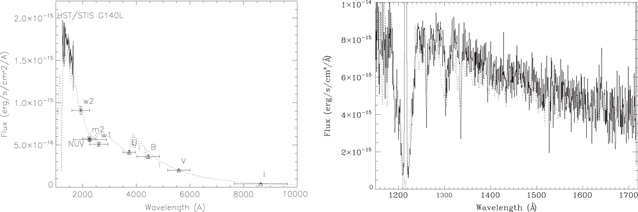
Figure 2. Left figure: the Zaritsky et al. (2004) field star UBVI photometry, the GALEX NUV data, quiescent Swift/UVOT w2, m2, and w1 photometry, and the last HST/STIS G140 L spectrum. The best fit is with a 15,000 K, log(g) = 4 Kurucz (1979) model atmosphere (dotted line). The model has been dereddened with E(B−V) = 0.15 mag (Dutra et al. 2001) and scaled by  where rstar = 3.8
  and D = 48 kpc. Right figure: comparison of the last HST/STIS G140 L spectrum (solid line; dereddened by E(B−V) = 0.15) and an IUE spectrum (SWP 15537) of the B3 V star ρ Aur (dotted line) dereddened by E(B−V) = 0.007 and scaled only by the distance difference (162 pc/48 kpc)2.
Download figure:
Standard image High-resolution imageThe angular separation between LMC 2012 and this field star is of order 023. The field star is not likely associated with the LMC 2012 system as an offset of 0.2 arcsec at the LMC distance corresponds to a minimum separation of ∼104 AU assuming both are coplanar. This is far too great for Roche lobe mass transfer and Krticka (2014) finds that B stars with effective temperatures of 15,000 K do not have any significant line driven mass loss that could effectively transfer material from the field star to the WD.
3. THE PAN-CHROMATIC DATA SET
3.1. Swift UV and X-Ray Data
Swift is a revolutionary facility for studying novae (see Schwarz et al. 2011, for details). Its three instruments cover the γ-ray (BAT), X-ray (XRT), plus UV and optical (UVOT) bandpasses. The XRT has superb soft X-ray response (Burrows et al. 2005) which makes it ideal for observing the Super-Soft-Source (SSS) phase of novae. The UVOT provides coincident UV/optical six filter photometry or low resolution grism spectroscopy (Roming et al. 2005). LMC 2012 was not detected by the BAT but an extensive data set exists from the numerous UVOT and XRT detections which are described below.
3.1.1. Swift UVOT
Swift obtained 74 uvm2 band ( = 2246 Å, FWHM = 498 Å) observations of LMC 2012 with the UVOT instrument from D1.2 until D671. There were also 12 uvw2 band (
 = 1928 Å, FWHM = 657 Å) and nine uvw1 band (
 FWHM = 693 Å) observations which were only obtained early on D1.2 and later during the observations after D300. The UVOT photometry is provided in Table 2 while the uvm2 light curve is shown in Figure 3.
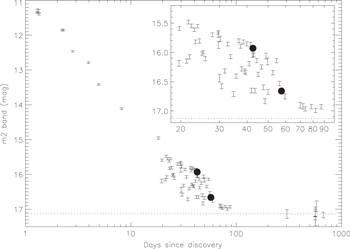
Figure 3. Swift/UVOT uvm2 band ( = 2246 Å) light curve of LMC 2012. The filled circles are the derived uvm2 band magnitudes from the HST spectra. The dotted line is the mean magnitude from the post D300 photometry derived from the field star. The inset expands on the significant short-term variability in the light curve between D20 and D60.
Download figure:
Standard image High-resolution imageTable 2. UV, Optical, and IR Photometry
 a a |
MJD | Mag | σ | Source |
| (days) | (days) | (mag) | (mag) | |
| m2 band | ||||
| 1.292 | 56013.689 | 11.297 | 0.051 | Swift/UVOT |
| 1.338 | 56013.735 | 11.309 | 0.051 | Swift/UVOT |
| B band | ||||
| 0.597 | 56012.994 | 11.900 | 0.002 | SMARTS |
| 1.040 | 56013.437 | 12.569 | 0.048 | AAVSO |
| V band | ||||
| 0.584 | 56012.981 | 11.985 | 0.007 | AAVSO |
| 1.044 | 56013.441 | 12.674 | 0.009 | AAVSO |
| R band | ||||
| 0.598 | 56012.995 | 11.278 | 0.002 | SMARTS |
| 1.047 | 56013.444 | 11.841 | 0.007 | AAVSO |
| I band | ||||
| 0.596 | 56012.993 | 10.932 | 0.003 | SMARTS |
| 1.053 | 56013.450 | 11.616 | 0.023 | AAVSO |
| J band | ||||
| 0.596 | 56012.993 | 10.407 | 0.027 | SMARTS |
| 1.618 | 56014.015 | 11.867 | 0.051 | SMARTS |
| H band | ||||
| 0.596 | 56012.993 | 9.883 | 0.019 | SMARTS |
| 1.618 | 56014.015 | 11.566 | 0.039 | SMARTS |
| K band | ||||
| 0.596 | 56012.993 | 9.369 | 0.024 | SMARTS |
| 1.618 | 56014.015 | 10.827 | 0.048 | SMARTS |
aWhere t0 is the discovery date, 2012 March 26.397 UT (MJD 56012.897).
Only a portion of this table is shown here to demonstrate its form and content. Machine-readable and Virtual Observatory (VO) versions of the full table are available.
Download table as: Machine-readable (MRT)Virtual Observatory (VOT)Typeset image
Swift observed LMC 2012 on five of the first eight days after discovery. These initial observations revealed that the uvm2 light curve declined 0.4 mag days−1. For the next 10 days, the nova could not be observed by Swift due to pointing constraints. When observations resumed LMC 2012 was a variable UV source with an ∼0.3 amplitude modulation superimposed on a declining light curve. It faded from uvm2 = 15 to uvm2 = 17 mag between D20 and D60. The amplitude of the oscillations was roughly constant from D20 through D50. From D50 to D60 the amplitude appears to have decreased to ∼0.15 mag but there were only four observations during this time. No further significant decline was seen until D90. When the same field was subsequently observed after D303 the detected source was approximately 0.2 mag fainter and within the uncertainty remained constant at 17.13 mag. The averaged uvm2 magnitude is shown as a dotted line in Figure 3 and represents the UV contribution of the field star. Figure 3 suggests that LMC 2012 dominated the field star prior to D100.
3.1.2. XRT
Swift observations of LMC 2012 began on D1.3 and continued for over 670 days. The XRT spectra were extracted for each individual observation using the latest version of the Swift software (HEASOFT 6.15.1 and the v014 calibration file for the PC RMF). These had typical exposure times of ∼1 ks, with one or two observations occurring most days between D18 and D54, and then once every 2–5 days until D87. All the data were collected using Photon Counting mode and circular regions were used for both source and background spectral extraction. If the source count rate was above about 0.6 count s−1, the core of the point-spread function was excluded in order to avoid pile-up. An 8 pixel excluded radius was used until D50. After that, as the nova faded, it was reduced to 5 pixels and then to 0 after D55. Event grades 0–12 were used for the timing analysis (Section 4.1) but only grade 0 were used for the spectral fitting (Section 4.2) to minimize residual pile-up.
Figure 4 shows the 0.3–10 keV XRT count rates and hardness ratios around the epoch when it was X-ray active. The data are provided in Table 3. The upper limits (3σ) and detection uncertainties (1σ), when the count rate was <0.01 ct s−1, were calculated using Bayesian statistics.
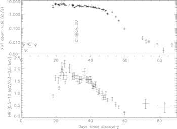
Figure 4. Swift/XRT 0.3–10 keV count rate (top) and hardness ratio ((0.5–10 keV/0.3–0.5 keV); bottom) evolution. Upper limits (3σ) to the count rate (top) are indicated by downward arrows. The time of the Chandra visit is shown to guide the eye.
Download figure:
Standard image High-resolution imageTable 3. Swift/XRT 0.3–10 keV Count Rate and Hardness Ratio
 a a |
MJD | CR |
 a a |
MJD | HRb |
|---|---|---|---|---|---|
| (days) | (days) | (ct s-1) | (days) | (days) | |
| 1.315 | 56013.715 | <0.008 | ⋯ | ⋯ | ⋯ |
| 2.525 | 56014.922 | <0.003 | ⋯ | ⋯ | ⋯ |
| 3.953 | 56016.352 | <0.009 | ⋯ | ⋯ | ⋯ |
| 4.957 | 56017.355 | <0.008 | ⋯ | ⋯ | ⋯ |
| 8.162 | 56020.559 | <0.008 | ⋯ | ⋯ | ⋯ |
| 18.217 | 56030.613 | 3.17 |
⋯ | ⋯ | ⋯ |
| 19.614 | 56032.012 | 5.03 |
19.649 | 56032.047 | 1.62
|
| 19.682 | 56032.082 |

|
|||
| 21.220 | 56033.617 |

|
21.220 | 56033.617 | 1.533
|
| 21.617 | 56034.016 |

|
21.751 | 56034.148 | 1.21
|
| 21.885 | 56034.281 | 4.43 |
|||
| 22.362 | 56034.762 | 5.67 |
22.362 | 56034.762 | 1.73
|
| 23.028 | 56035.426 | 5.35 |
23.028 | 56035.426 | 1.87
|
| 23.295 | 56035.695 | 5.34 |
23.295 | 56035.695 | 2.11
|
| 23.822 | 56036.219 | 5.28 |
23.822 | 56036.219 | 1.97
|
| 24.287 | 56036.688 | 5.87 |
24.287 | 56036.688 | 1.72
|
| 24.957 | 56037.355 | 5.03 |
24.957 | 56037.355 | 2.19
|
| 25.294 | 56037.691 | 4.45 |
25.294 | 56037.691 | 1.46
|
| 25.826 | 56038.227 | 4.50 |
25.826 | 56038.227 | 1.71
|
| 27.829 | 56040.227 | 4.75 |
27.829 | 56040.227 | 2.02
|
| 29.566 | 56041.965 | 4.92 |
29.566 | 56041.965 | 1.68
|
| 29.627 | 56042.027 | 4.26 |
29.935 | 56042.332 | 1.70
|
| 29.694 | 56042.094 | 4.12 |
|||
| 30.029 | 56042.426 | 4.18 |
|||
| 30.242 | 56042.641 | 4.67 |
|||
| 30.700 | 56043.098 | 3.16 |
30.700 | 56043.098 | 1.71 |
| 31.702 | 56044.102 | 3.77 |
31.702 | 56044.102 | 1.61 |
| 32.699 | 56045.098 | 4.41 |
⋯ | ⋯ | ⋯ |
| 32.705 | 56045.102 | 4.10 |
32.705 | 56045.102 | 1.61
|
| 33.702 | 56046.102 | 4.20 |
⋯ | ⋯ | ⋯ |
| 33.708 | 56046.105 | 3.54 |
33.708 | 56046.105 | 1.55
|
| 34.708 | 56047.105 | 3.77 |
34.708 | 56047.105 | 1.56
|
| 35.709 | 56048.109 | 3.55 |
35.709 | 56048.109 | 1.74
|
| 36.778 | 56049.176 | 4.16 |
36.778 | 56049.176 | 1.87
|
| 37.446 | 56049.844 | 4.15 |
37.446 | 56049.844 | 1.54
|
| 37.846 | 56050.246 | 3.74 |
37.846 | 56050.246 | 1.56
|
| 38.448 | 56050.848 | 3.61 |
38.448 | 56050.848 | 1.54
|
| 38.915 | 56051.312 | 3.48 |
38.915 | 56051.312 | 1.53
|
| 39.451 | 56051.848 | 3.50 |
39.451 | 56051.848 | 1.56
|
| 39.918 | 56052.316 | 3.35 |
39.918 | 56052.316 | 1.55
|
| 40.452 | 56052.852 | 3.38 |
40.452 | 56052.852 | 1.49
|
| 40.918 | 56053.316 | 3.23 |
40.918 | 56053.316 | 1.30
|
| 41.521 | 56053.918 | 3.45 |
41.521 | 56053.918 | 1.27
|
| 41.921 | 56054.320 | 3.07 |
41.921 | 56054.320 | 1.26
|
| 42.522 | 56054.922 | 3.13 |
42.522 | 56054.922 | 1.35
|
| 42.857 | 56055.254 | 3.25 |
42.857 | 56055.254 | 1.32
|
| 43.524 | 56055.922 | 2.72 |
43.524 | 56055.922 | 1.16
|
| 44.394 | 56056.793 | 2.86 |
44.394 | 56056.793 | 1.04
|
| 45.008 | 56057.406 | 2.62 |
45.008 | 56057.406 | 1.08
|
| 46.597 | 56058.996 | 2.27 |
46.597 | 56058.996 | 0.99
|
| 47.532 | 56059.930 | 2.17 |
47.532 | 56059.930 | 0.81
|
| 48.333 | 56060.730 | 1.73 |
48.333 | 56060.730 | 0.81
|
| 48.804 | 56061.203 | 1.88 |
48.804 | 56061.203 | 0.93
|
| 49.670 | 56062.066 | 1.15 |
49.774 | 56062.172 | 0.71
|
| 49.875 | 56062.273 | 1.03 |
|||
| 52.542 | 56064.941 | 1.43 |
52.542 | 56064.941 | 0.75
|
| 54.546 | 56066.945 | 0.65 |
54.546 | 56066.945 | 0.54
|
| 56.282 | 56068.680 | 0.34 |
56.282 | 56068.680 | 0.43
|
| 59.626 | 56072.023 | 0.09 |
59.626 | 56072.023 | 0.20
|
| 69.945 | 56082.344 | 0.02 |
71.749 | 56081.648 | 0.58
|
| 71.953 | 56084.352 | 0.01 |
|||
| 73.683 | 56086.082 | 0.01 |
|||
| 78.521 | 56090.918 | 0.01 |
⋯ | ⋯ | ⋯ |
| 82.205 | 56095.102 | 0.003 |
82.966 | 56095.363 | 0.51
|
| 87.145 | 56099.543 | 0.006 |
⋯ | ⋯ | ⋯ |
| 303.224 | 56315.621 | <0.03 | ⋯ | ⋯ | ⋯ |
| 562.965 | 56575.364 | <0.01 | ⋯ | ⋯ | ⋯ |
| 563.254 | 56575.651 | <0.02 | ⋯ | ⋯ | ⋯ |
| 564.305 | 56576.702 | <0.01 | ⋯ | ⋯ | ⋯ |
| 579.227 | 56591.626 | <0.04 | ⋯ | ⋯ | ⋯ |
| 671.512 | 56683.910 | <0.01 | ⋯ | ⋯ | ⋯ |
Notes. On some dates the HR was determined by summing the source counts from multiple exposures.
aWhere t0 is the discovery date, 2012 March 26.397 UT (MJD 56012.897). bWhere HR = (0.5–10 keV)/(0.3–0.5 keV).There was no X-ray detection in the first five observations through D8.2 when the UVOT recorded its rapid UV decline. Once LMC 2012 was no longer pointing constrained, monitoring began again and the next Swift observation on D18.15 detected a bright and soft X-ray source with a count rate of 4.12 ± 0.08 ct s−1.
LMC 2012 reached a maximum X-ray count rate of ∼6 ct s−1 on D19.7. The hardness ratio, centered on the soft component, (HR = (0.5–10 keV)/(0.3–0.5 keV)) at maximum was about 2 at D25. This hardness ratio indicates a soft X-ray spectrum consistent with hot thermal emission at kT ∼90 eV (see Section 4.2). The X-ray source remained approximately constant in both the flux and hardness ratio over the next 20 days, after which it began declining in both. Figure 5 shows the spectral evolution using the XRT spectra obtained on D25, D42 and D56. By D80 the XRT count rate had declined by a factor of 100 and the nova had become a significantly softer X-ray source than that seen around D60 as the spectral energy distribution shifted to cooler temperatures. Additional Swift observations obtained starting on D303 and ending on D671 detected no X-ray source.
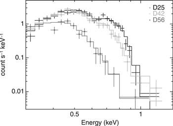
Figure 5. Swift/XRT spectra of LMC 2012 obtained at X-ray maximum (D25; pluses) and nearly coincident with the first (D42; Xs) and second (D56; filled circle) HST observations. The spectra are fit with the models described in Figure 14 but also include an optically thin MEKAL model to account for the counts above 1 keV. The spectral evolution is consistent with a fading and cooling source.
Download figure:
Standard image High-resolution imageLMC 2012 entered its SSS phase after D8 and before D18 so we set the SSS turn-on time,  , to 13 ± 5 days. This is a very rapid turn-on and implies either that very little mass was expelled or the ejecta were significantly aspherical (Shore et al. 2013) since the X-ray turn-on is due to the decrease in the optical depth of the ejecta, for a given ejection velocity. An upper limit on the ejected mass of order 10−6
  is suggested from the expansion velocity and
  based on the simple homogenous and uniformly expanding shell models of Schwarz et al (2011, see their Figure 8). This low mass is very similar to those of fast recurrent novae (for example, see Schaefer 2011; Anupama 2013).
Based on its X-ray light curve and hardness ratio, LMC 2012 ended its SSS phase around D50. The SSS duration is inversely proportional to the WD mass and a short timescale implies a high mass WD (Starrfield et al. 1991). Compared to the turn-off times,  of Table 5 in Schwarz et al. (2011), LMC 2012 had one of the fastest X-ray turn-off times detected. Figure 9 in Schwarz et al. (2011) shows how rare this rapid a turn-off is relative to the Galactic novae with SSS detections. A
  days is similar to recurrent novae such as RS Oph (60 days; Osborne et al. 2011), V745 Sco (∼5 days; Osborne et al. 2014), and U Sco (34 days; Schaefer et al. 2010) plus the suspected recurrents V2491 Cyg (44 days; Page et al. 2010), V2672 Cyg (28 days; Schwarz et al. 2011), and V407 Cyg (30 days; Schwarz et al. 2011). There are also novae in M31 with similar rapid turn-off times such as the recurrent M31 2008-12a (
 days) (see Henze et al. 2014, for details).
Henze et al. (2014) compiled four correlations between X-ray and nova properties for M31 novae. That galaxy is ideal for these sorts of comparisons since the uncertainties in the distance are effectively eliminated and there are sufficient numbers detected each year to create a statistically viable sample. These observational relations (their Equations (4)–(7)) give the  versus
  ,
,  versus the effective blackbody temperature,
  versus
  , and
, and  versus
  relationships. For LMC 2012 we adopted
  = 13 days,
  = 50 days, kT = 86 eV from the Swift/XRT model fits, vexp = 5000 km s−1 from the estimates from the early P-Cygni absorption lines, and
  days from Figure 1. The observed X-ray behavior of LMC 2012 is well described by these equations. Its predicted
  times from the Henze et al. (2014) Equations (4) and (5) are 62
 and 71
 days, respectively. The derived
  times for Equations (6) and (7) are both ∼14
 days.
days.
3.2. Chandra X-Ray Spectroscopy
A Director’s Discretionary Time observation of LMC 2012 was obtained with the Low Energy Transmission Grating (LETG) and High Resolution Camera Spectroscopic detector. Observation ID 14426 commenced at UT April 26, 21:56 (D32.016) and ended at UT 04:00 on 2012 April 27 (D32.270), and had a net exposure time of 20 ks. Data were obtained from the Chandra archive13 and were reprocessed using CIAO and calibration database versions 4.6.1. Effective areas and instrument response files were generated using standard CIAO procedures.
The combined plus and minus order spectra are shown in Figure 6. Initial reports were provided by Takei et al. (2012) and Orio et al. (2012). The spectrum was that of a soft X-ray source with some emission and absorption lines. It was exceptionally hot and similar to high resolution spectra of RS Oph in the supersoft phase (Ness et al. 2007), which had an estimated effective temperature of about 106 K (Osborne et al. 2011). The absorption lines were weaker in LMC 2012 than in the RS Oph spectra. This may be due to the lower metallicity of the LMC, but this hypothesis requires detailed model atmosphere analysis to confirm.
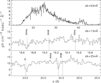
Figure 6. Full Chandra DDT spectrum (D32) rebinned to 0.063 Å (top panel). The middle and bottom panels show the absorption and emission features around 19 and 24 Å, respectively. Various lines are labeled and have been Doppler shifted by −4400 km s−1. The middle panel spectrum is rebinned to 0.013 Å while the bottom panel spectrum is rebinned to 0.025 Å.
Download figure:
Standard image High-resolution imageThe strongest emission lines are the  (Ly α-like) transitions of the hydrogenic ions N vii
  and O viii
  . No prominent features due to carbon were seen. The N vii and O viii lines exhibited P-Cygni-like absorption, blueshifted by approximately 4400 km s−1. While this absorption shift is consistent with earlier optical spectroscopic data, these features could also be a chance superposition of absorption and emission lines. The spectral regions around the N viiiα line and N vii lines are illustrated in the middle and bottom portions of Figure 6.
In Figure 7 we show the total count and spectral evolution of the Chandra/LETG observation. The observation was divided into 41 adjacent time intervals, each of 500 s duration, from which time-filtered spectra were extracted in photon flux units. These spectra are arranged in the central time map with time running down, wavelength across, and brightness encoded with the color scheme outlined in the top right corner. The light curve shows a slow and small increase starting at ∼4 hr after the start of the observation. This increase seems to be accompanied by a limited increase in the Wien tail, shortward of ∼19 Å which is close to the N vii ionization edge at 18.6 Å. The spectrum extracted between 0.4 and 3.2 hr into the observation (blue) contains a slightly deeper absorption feature at this wavelength, and the higher flux shortward of 19 Å in the spectrum extracted later between 4.9 and 5.5 hr (red) might be due to reduced absorption caused by N vii.
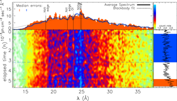
Figure 7. Spectral time map of the Chandra observation. The X-ray light curve, extracted from the zeroth order, is shown in the right panel, rotated by 90°. Along the same, downward, time axis, the spectral evolution is illustrated as a brightness color map in the central panel in which wavelength runs across (for meaning of color scheme, see top right). Along the same wavelength axis, selected spectra are shown in the top panel, with the red and blue colors corresponding to the shaded areas in the right panel and dashed horizontal lines in the central panel, which mark the time intervals from which the spectra were extracted. The median error bars for each spectra are given with the red and blue vertical lines in the top left corner. In addition to the two individual spectra, the average spectrum and a blackbody fit are shown with black and solid and dotted lines, respectively. An increase in count rate by ∼25% coincides with higher emission shortward of the NV ii absorption edge at 18.6 Å, indicating that reduced absorption causes the higher count rate (see text).
Download figure:
Standard image High-resolution imageExploration of the full range of model atmosphere parameters to provide detailed estimates of the element abundances and mass loss rate of LMC 2012 requires extensive and detailed computations that are beyond the scope of the present work. The goal here is instead to use the Chandra/LETG spectrum to support the Swift data set, obtain an approximate description of the global spectral energy distribution, and characterize the ionizing flux shortward of the Lyman edge for the photoionization modeling.
3.3. HST/STIS Spectroscopy
After discovery, LMC 2012 was selected as the ToO target of a cycle 19 program (GO-12484) to obtain high resolution UV spectroscopy at three separate times during its evolution. The HST observation log of the observations is presented in Table 4.
Table 4. HST Observation Log
| Exp. ID | UT Start Time | MJD Start Time |
 a a |
Total Exp. | Grating | Aperture | Range | Int. Flux |
|---|---|---|---|---|---|---|---|---|
| (hh:mm:ss) | (days) | (s) | (days) | (″) | (Å) | erg cm−2 s−1 | ||
| Visit 1: 2012-05-07-08 | ||||||||
| Obtg01010 | 23:30:15 | 56055.479 | 42.58 | 724 | E140 M | 0.2X0.2 | 1140–1735 | 1.7 × 10⁻¹² |
| Obtg01020 | 23:48:24 | 56055.492 | 42.59 | 724 | E230 M | 0.2X0.2 | 1574–2382 | 9.5 × 10 −14b |
| Obtg01030 | 00:05:53 | 56055.504 | 42.61 | 724 | E230 M | 0.2X0.2 | 2303–3133 | 9.9 × 10 −13c |
| Visit 2: 2012-05-23 | ||||||||
| Obtg02010 | 07:30:18 | 56070.313 | 57.41 | 690 | G140 L | 52X0.2 | 1140–1735 | 1.0 × 10⁻¹² |
| Obtg02020 | 07:47:55 | 56070.325 | 57.43 | 690 | G230 L | 52X0.2 | 1570–3180 | 7.9 × 10⁻¹³d |
| Obtg02030 | 08:03:01 | 56070.335 | 57.44 | 780 | G430 L | 52X0.2E1 | 2900–5700 | 1.0 × 10⁻¹² |
| Visit 3: 2012-07-17 | ||||||||
| Obtg99010 | 04:13:43 | 56125.176 | 112.27 | 2746 | G140 L | 0.2X0.2 | 1140–1735 | 9.2 × 10⁻¹³ |
aWhere t0 is the discovery date, 2012 March 26.397 UT (MJD 56012.897). bFrom 1735 to 2350 Å. cFrom 2350 to 3130 Å. dFrom 1735 to 3130 Å.
Download table as: ASCIITypeset image
Due to pointing constraints, the first visit could not be scheduled until D42. This observation used the STIS medium echelle grating to obtain coverage from 1150 to 3100 Å. Surprisingly, only one emission line, N v (1240 Å), was detected, see Figure 8. The continuum was relatively flat with an integrated UV flux from 1140 to 3130 Å of 2.8 × 10⁻¹² erg cm −2 s−1 (uncorrected for extinction).
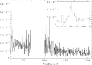
Figure 8. Highest S/N portions of the UV spectrum from D42 rebinned to 2 Å resolution. The only prominent line is N v at 1240 Å which is shown in greater detail in the inset.
Download figure:
Standard image High-resolution imageFor the second visit on D57 the low resolution grating was used since the nova was already too faint to observe with the echelle. The integrated 1140–3130 Å UV flux had decreased to 1.8 × 10⁻¹² erg cm−2 s−1. An optical grating exposure was also included since the source could no longer be observed with the SMARTS spectrograph. Except for N v, no emission lines were detected in the UV and optical spectra. In addition, the optical spectrum showed a Balmer discontinuity that had not been present before which was likely due to contamination from the field star. Figure 9 shows the combined D57 UV and optical spectra.
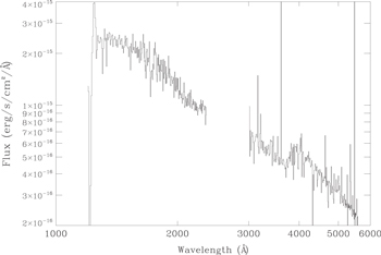
Figure 9. STIS G140L, G230L, and G430L spectra binned to 5 Å resolution from D57. The only detected line is again N v at 1240 Å.
Download figure:
Standard image High-resolution imageWith the continuing decline in the light curve, the entire orbit allotment was used for a single low resolution FUV exposure on D112. Unfortunately, neither the rapid decline nor the presence of the field star was anticipated prior to the observation, and HST's acquisition locked on the field star which was by then the brightest source in the field.
3.4. SMARTS Optical and Near-IR Data
LMC 2012 was extensively observed spectroscopically and photometrically with the SMARTS telescopes at Cerro Tololo (see Walter et al. 2012 for details). The spectroscopic observations were obtained between D0.6 and D45.6. LMC 2012 was photometrically monitored between D0.6 and D635. The cadence was initially daily but decreased as the source faded.
3.4.1. Photometry
We obtained 250 photometric observations in BVRI/JHK from SMARTS. The optical photometry is supplemented with 54 early time CCD BVRI observations from the AAVSO. The optical and NIR photometry is also given in Table 2.
The mean optical rate of decay in the B and V bands was about 0.34 mag days−1 from D2 through D10 but about 0.04 mag days−1 from D10 through D40. The early decline rate was similar to that observed in the UV uvm2 filter (Section 3.1.1) and the steady optical decay also gave way to a variable and oscillatory behavior from D11 to D50.
After D80 the measured photometry was constant at about V = 18.3 and B = 18.2. This is consistent with the BV photometry of Zaritsky et al. (2004) for the field star and indicates that LMC 2012 had faded below the optical brightness of the field star after only 3 months.
There was no evidence in the optical or NIR light curves for any dust formation which is consistent with fast novae rarely forming extensive dust shells (Gehrz et al. 1998).
3.4.2. Spectroscopy
We obtained 17 optical spectra from D0.6 through D45.6, see Table 5. Unfortunately, LMC 2012 was too faint to observe with the 1.5 m telescope after conjunction with the Sun.
Table 5. SMARTS Spectral Observation Log
| UT Start Time | MJD | |||
|---|---|---|---|---|
| (YYYY-mm-ddThh: | Start Time |
 a
a
|
Exp. | Range |
| mm:ss) | (days) | (days) | (s) | (Å) |
| 2012-03-26T23:55:54.4 | 56012.997 | 0.60 | 900 | 5620–6930 |
| 2012-03-27T22:40:01.1 | 56013.944 | 1.55 | 900 | 3642–5412 |
| 2012-03-28T23:37:34.7 | 56014.984 | 2.60 | 1200 | 5620–6930 |
| 2012-03-30T23:28:13.6 | 56016.978 | 4.58 | 1200 | 5620–6930 |
| 2012-04-01T23:53:07.8 | 56018.995 | 6.60 | 1200 | 3642–5412 |
| 2012-04-02T23:30:22.9 | 56019.979 | 7.58 | 1200 | 3250–9400 |
| 2012-04-05T20:20:10.5 | 56022.847 | 10.45 | 1200 | 3642–5412 |
| 2012-04-06T23:38:40.7 | 56023.985 | 11.59 | 2700 | 5620–6930 |
| 2012-04-07T23:34:19.3 | 56024.982 | 12.58 | 1200 | 3642–5412 |
| 2012-04-08T23:20:47.0 | 56025.973 | 13.57 | 2700 | 3642–5412 |
| 2012-04-12T20:37:01.3 | 56029.859 | 17.46 | 2700 | 5620–6930 |
| 2012-04-14T23:21:57.2 | 56031.974 | 19.58 | 1500 | 3870–4540 |
| 2012-04-15T20:55:30.7 | 56032.872 | 20.47 | 1800 | 3642–5412 |
| 2012-04-16T23:32:48.5 | 56033.981 | 21.58 | 1800 | 5620–6930 |
| 2012-04-18T23:27:37.3 | 56035.978 | 23.58 | 2700 | 3250–9400 |
| 2012-04-24T21:20:00.7 | 56041.889 | 29.49 | 3600 | 3250–9400 |
| 2012-05-10T23:25:35.7 | 56057.976 | 45.58 | 1800 | 3250–9400 |
aWhere t0 is the discovery date, 2012 March 26.397 UT (MJD 56012.897).
Download table as: ASCIITypeset image
The first (red) spectrum was obtained on D0.6. The Hα line showed a P-Cygni absorption profile due to the wind/expanding envelope at velocities ranging from −4500 to −5500 km s−1 similar to the description given in Prieto (2012). No P-Cygni absorption components were observed after D2.6. The initial Hα emission line showed a FWZI of 247 Å (11,300 km s−1), an emission equivalent width of 308 Å and integrated flux of 1.6 × 10⁻¹¹ erg s−1 cm−2. Extremely broad lines, ∼5000 km s−1, of N ii (5755 Å) and He i (5876 Å) were also present in the early red spectra.
The first blue spectrum, D1.5, showed very bright emission at wavelengths shorter than about 4100 Å, perhaps due to the confluence of the very broad higher Balmer lines. This, and the red spectrum obtained on D2.6, is shown in Figure 10. The combined spectrum is similar to the earliest spectra of the very fast ONe novae LMC 1990 #1 (Williams et al. 1991) and V4160 Sgr (Williams et al. 1994).
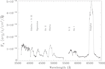
Figure 10. Earliest combined blue and red SMARTS optical spectrum of LMC 2012 from the epoch D1.5–D2.6. The point-to-point uncertainties are of order 1.5 × 10⁻¹⁵ erg s−1 cm−2 Å−1. Prominent lines are labeled.
Download figure:
Standard image High-resolution imageTo see how the expansion velocity in LMC 2012 compared to other novae, the large, uniform sample of 52 Galactic and Magellanic Cloud novae with measured FWHMs obtained near visual maximum from Schwarz et al. (2011) was used. Prieto (2012) measured the FWHM of the Hα line near maximum to be 125 Å (5700 km s−1). Only three novae, U Sco, V2478 Oph and V2672 Oph, had greater FWHM at this time in the outburst. All three are recurrent or suspected recurrent novae. Using the same criteria in the LMC-only sample of Shafter (2013), the FWHM of LMC 2012 is only exceeded by two novae, LMC 1990 #1 and LMC 1990 #2. The former was a very fast ONe type (Vanlandingham et al. 1999) and the latter was a recurrent nova (LMC 1968; Shore et al. 1991; Williams et al. 1991).
By D2.6 the Hα line had the distinctive tri-partite line profile common in U Sco-like recurrent novae. The central peak was the strongest of the three peaks. Four days later the blue spectrum was no longer dominated by the Balmer lines, but by the Bowen N iii lines. The strongest line in the low dispersion optical spectrum on D7.6 was (Ne v) (3426 Å), with the Bowen blend a close second. He ii (4686 Å) was not present on D6.6, but was strong on D10.4. He ii may have been present, but heavily blended, on D7.6. He ii was narrow (∼25 Å or 1600 km s−1), and was the strongest line in the blue spectrum by D13.6. A review of the optical spectra in Walter et al. (2012) and the X-ray light curves in Schwarz et al. (2011) show that in fast novae, the narrow He ii (4686 Å) emission appears before the emergence of soft X-rays. The evolution of the narrow He ii line in LMC 2012 is consistent with the SSS appearance prior to D18.
By D11.6 there was some excess emission around 6400 Å that could be associated with (Fe x) (6375 Å). This emission was present in the red spectra until D29.5. If this excess were due to the actual emergence of this emission line, it was consistent with the emergence of the SSS on day D18 (Krautter et al. 1984; Schwarz et al. 2011). Figure 11 shows the SMARTS spectrum on D23.6. By that time the nova had faded sufficiently that only He ii, Hα, and possibly (Ne v) and (Fe x) were still visible. In the last spectrum on D45.6 there were no obvious emission lines.
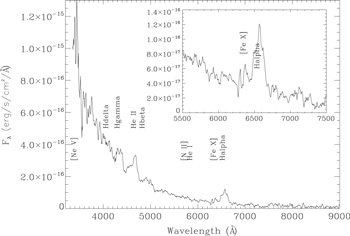
Figure 11. Full SMARTS optical spectrum of D23.6, obtained near the peak of the SSS emission. Prominent lines are labeled.
Download figure:
Standard image High-resolution image4. MODELING THE SSS EVOLUTION
4.1. Period Analysis
A Lomb–Scargle periodogram was formed from the 50 Swift uvm2 photometric measurements obtained from D19 to D60 after subtraction of a first order polynomial to remove the secular decline. A peak in the periodogram at 1.2473 cycles day−1 (Figure 12), in excess of the 99.9% confidence level of 11.0 and corresponding to a period  hr, is derived with the method of Horne & Baliunas (1986) under the reasonable assumption of even sampling. The error is derived from a least squares sine fit to the de-trended data with the photometric errors increased artificially to allow a fit with a reduced chi squared of unity. The periodogram also shows aliases with the Swift orbital period, as expected from the convolution of the source signal with the window function of the data, and a peak at 3.17 cycles days−1 with a power corresponding to ∼90% confidence; these peaks are not present in a periodogram of the data set with the 19.24 hr modulation subtracted, confirming that they are not intrinsic to the source. The uvm2 light curve folded at the 19.24 hr period is shown in Figure 13; modeled with a sine function, the amplitude is 0.306 ± 0.031 mag. A periodogram of the D19–60 XRT 0.3–10 keV X-ray light curve de-trended with a second order polynomial shows no significant power at the UV period. We find the 90% upper limit to the amplitude of any modulation of the X-rays at the UV period to be 15%.
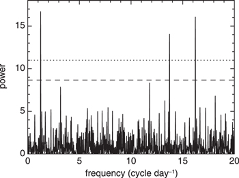
Figure 12. Lomb–Scargle periodogram of the Swift uvm2 photometry obtained between D19 and D60 after subtraction of a first order polynomial, with the 99.0% and 99.9% confidence levels shown. A significant peak is seen at 1.2473 cycles day−1 (=19.24 hr); other strong peaks are aliases of this with the Swift orbital period (15 cycles day−1) and are not present when the source periodic modulation is subtracted from the data set.
Download figure:
Standard image High-resolution image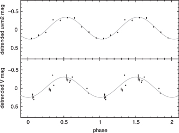
Figure 13. (Top) Swift uvm2 photometry obtained between D19 and D60 after subtraction of a first order polynomial folded at the 19.24 hr period; errors represent the standard deviation of the distribution of values in each 0.1 phase bin. (Bottom) The SMARTS V band photometry obtained between D19 and D60 after subtraction of a first order polynomial folded at the same period; errors are propagated. Solid curves represent the best sine fits.
Download figure:
Standard image High-resolution imageThe SMARTS light curve shows a modulation with the same period detected in the UV, although these data do not permit the independent detection of this period. The 19.24 hr period amplitudes in the BVRIJHK filters were 0.269 ± 0.007, 0.275 ± 0.009, 0.280 ± 0.011, 0.305 ± 0.019, 0.39 ± 0.31, 0.47 ± 0.26, and 0.76 ± 0.23 mag, respectively over D19–60; 90% confidence errors are given. The SMARTS V band photometry folded at the 19.24 hr period is also shown in Figure 13.
The origin of the modulation is not known but it is likely orbital in nature. Even in a long period system, the secondary would be tidally locked and strongly irradiated around the substellar point by the hot WD. In an inclined system (see Section 4.3.1) the distended and illuminated lobe would produce variations in the UV through NIR with amplitudes similar to what was observed. Conversely, the X-ray light curve is constant (Sections 3.1.2 and 3.2) as the X-rays are emitted from the WD atmosphere which is not modulated by the orbital motion.
While it is possible that observed UV and optical variability could also come from illumination and heating of a warped accretion disk, we discount this possibility as it would not account for the lack of similar modulation in the X-ray data sets. In addition, an accretion disk would have to either survive the initial nova explosion or reform very quickly even as the WD was at peak luminosity and temperature. More exotic scenarios may also be at work but an illuminated secondary is the simplest explanation that fits all the available data and thus is favored in the subsequent analysis. Confirmation of a 19.24 hr orbit will require observations during quiescence.
4.2. Modeling the X-Ray Spectral Evolution
We use the extensive Swift XRT data set to model the entire X-ray evolution during the outburst in LMC 2012. Initially, the Swift X-ray spectra were modeled using a combination of a blackbody or a plane-parallel, static, non-local thermal equilibrium atmosphere component14 (Rauch 2003; Rauch et al. 2010) to parameterize the soft emission, plus a single temperature optically thin thermal plasma to account for the emission at higher energies. Although a gross simplification of the underlying physics, in low resolution X-ray spectra such as the XRT, blackbody models are sometimes used to characterize the temperature and luminosity changes of the soft emission. Blackbody fits, however, can underestimate the true temperature and generally overestimate the bolometric luminosity (Heise et al. 1994). A more realistic treatment of the physics comes from the use of hydrostatic model atmospheres which can, unlike blackbodies, sucessfully fit the higher resolution X-ray spectra. For LMC 2012, the C-stat values for the blackbody fits were significantly worse than for the model atmosphere fits and thus the blackbody fits were not used in the analysis. In addition, the choice of model atmosphere did not significantly affect the fit to the data or the derived properties. Both the hard and soft model components were absorbed by a freely varying column. Luminosities were calculated assuming a distance of 48 kpc.
Figure 14 shows the results of the model atmosphere fits to the Swift X-ray data during the SSS phase. From D20 to D42 the X-ray spectra are well fit by models with a constant effective temperature of order 86 eV, ∼1 MK. The fitted model luminosities are not as well constrained with values between (1–10)×1038 erg s−1. Since the distance to the LMC is well known, an upper limit on the bolometric luminosity can be established from the Eddington limit for a 1.4  WD, i.e., ∼1 × 1038 erg s−1 cm−2. Excluding the models with the largest errors, the hydrogen column density evolution is compatible with
  2 × 1021 cm−2. This value is consistent with the external extinction along the line of sight of NH = 0.7 × 1021 cm−2 used to correct the field star photometry and FUV spectrum (E(B−V) = NH/4.8 × 1021 and E(B−V) = 0.15 mag Bohlin et al. 1978).
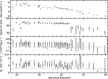
Figure 14. Model atmosphere fits to the Swift/XRT spectra during the time LMC 2012 was in the SSS phase. The top panel shows the XRT light curve on a linear scale. The next three panels give the best fit model atmosphere effective temperatures, bolometric luminosities, and NH parameters. The gray lines in the luminosity and NH panels represent a typical Eddington luminosity for a high mass WD (1 × 1038 erg s−1 and the extinction, 1.16 × 1021 cm−2, derived from the Chandra model fit, respectively.
Download figure:
Standard image High-resolution imageThe model sequence confirms that LMC 2012 was at its maximum effective temperature early in the Swift observations of the SSS phase and maintained a constant bolometric luminosity at about the Eddington limit for approximately 50 days. Figure 15 shows the combined XRT spectrum from the D18 to D50 data. The best fit had a model atmosphere temperature of 86.2 ± 0.3 eV and an optically thin MEKAL component temperature of 0.120 ± 0.007 keV. The model NH was 1.7 × 1021 cm−2 which is consistent with the typical LMC NH value (Welty et al. 2012).
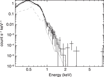
Figure 15. Total XRT spectrum from the combined D18–D50 observations. The best fit model atmosphere (dark dotted line) and MEKAL model (gray dashed line) are also shown.
Download figure:
Standard image High-resolution imageAs an additional check on the validity of the models used to fit the entire Swift/XRT data set, the Chandra/LETG spectra (plus and minus orders) were fitted with the same atmosphere grid model as described above. No additional components were included. The resulting parameters for the atmosphere component are consistent with those from the XRT data taken close in time, although the best fit absorption column from the grating spectra is lower, at (1.16 ± 0.03) × 1021 cm−2, compared to 1.7 × 1021 cm−2 from the combined Swift D18–50 data spectrum or the  × 1021 cm−2 from the D31.7 XRT spectrum, see Figure 16. While van Rossum (2012) shows that at wavelengths longer than 40 Å models are very sensitive to the choice of NH, the S/N in the Chandra spectrum is not of sufficient quality in this region to constrain NH further.
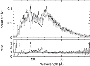
Figure 16. Chandra/LETG spectrum (D32; black and gray plus symbols are the plus and minus orders, respectively) and the best fit Rauch atmosphere model from the same grid as used in the Swift/XRT analysis. The best fit model atmosphere temperature to the LETG spectrum, 88.0 ± 0.3 eV, was similar to that derived for the lower resolution XRT spectrum obtained on D31.7, 87 eV. Note that the significant residuals in the model fit correspond to the strongest blueshifted lines which are not incorporated in the model.
Download figure:
Standard image High-resolution imageThe lack of any significant hard X-ray emission in LMC 2012 is surprising as most novae bright enough for X-ray observations have an early period of hard X-ray emission from shocks (e.g., see Schlegel et al. 2010; Schwarz et al. 2011; Chomiuk et al. 2014 for details). The shocks are thought to arise from either internal shocks within the ejecta or the ejecta running into pre-existing material such the wind from a red giant companion. Fitting another MEKAL component centered at KT = 5 keV improves the fit to the data above 1 keV in the combined spectrum shown in Figure 15. The 90% confidence upper limit on the bolometric flux of this new hard component is 8.2 × 10⁻¹⁴ (observed) or 1.3 × 10⁻¹³ (unabsorbed) erg cm−2 s−1. This is equivalent to bolometric luminosities of 9.8 × 1030 and 1.3 × 1031 erg s−1, respectively, at 48 kpc. This luminosity upper limit is significantly lower than the 1034–35 erg s−1 that is typically observed (Mukai et al. 2008; Metzger et al. 2014).
4.3. Modeling the Ejecta
4.3.1. Line Profile Fitting
To obtain an idea of the geometry of the ejecta, we modeled the optical Balmer lines using the Monte Carlo procedure described in Shore et al. (2013). Figure 17 shows two Hα profiles compared with the model parameters that were chosen to provide an approximate representation, consistent with the dynamics and profile evolution. A similar solution was obtained for the other Balmer lines. The model parameters are the relative shell thickness ( ) where R is the radius given by the maximum observed velocity during the earliest stages, the inner and outer angles of bipolar symmetric ejecta (
 ), and the inclination of the axis of the ejecta to the line of sight i. The displayed profiles were smoothed to 100 km s−1 to reduce the stochastic fluctuations and the line was assumed to be formed by recombination. We assumed a ballistic velocity law. For
  there is no central peak and multiple low velocity peaks are obtained if
  . Otherwise, with the ejecta appear to be bipolar with a moderately high inclination to the line of sight, subtending a solid angle of about 2π with respect to a spherical shell. No spherical solution is acceptable at any time and the inner angle appears to have decreased over time with increasing transparency. The same behavior has been found for other novae similarly modeled (e.g., Shore 2012; Ribeiro et al. 2013a, 2013b).
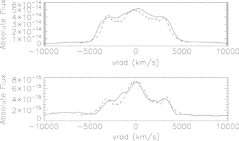
Figure 17. Simulation (dotted lines) of two Hα profiles from the SMARTS data (solid lines) using the Monte Carlo procedure from Shore et al. (2013). The top spectrum is D2.6, the bottom is from D11.6. The model parameters are vmax = 6500 km s−1,  = 0.3,
  ,
,  ,
,  . See text for details.
Download figure:
Standard image High-resolution image4.3.2. Photoionization Analysis
We used the Cloudy (Ferland et al. 2013) photoionization code to fit the pan-chromatic data set for four separate dates, D7.5, D29.5, D42, and D57. For a given set of input parameters, Cloudy solves the equations of thermal and statistical equilibrium and predicts both a continuum and emission line ratios. A Cloudy model for a nova requires a set of input parameters for the ejected shell and the photoionizing source. The source parameters are the luminosity and spectral energy distribution. The shell parameters are the geometry, structure, hydrogen density, and elemental abundances relative to hydrogen.
The Cloudy models require a large number of parameters so it is desirable to minimize the set either from the data or physical assumptions. For the ejecta, the inner and outer radii for LMC 2012 were assumed to be equal to minimum and maximum ejection velocities of 1000 and 5000 km s−1 times the number of days since discovery. The model filling and covering factors were set to 0.1 and 1, respectively, which are typical for similar photoionization analyses (see Schwarz et al. 2007, for examples). The radial variation of the ejecta number density was assumed to be (r/ri)−3 so that the mass is constant in the shell (ballistic expansion). After fixing the radii and ejecta structure, the only free–shell parameter that determines the ejecta mass is the hydrogen density at the inner radius, ri. The lack of emission lines in the later spectra means that the ejecta abundances could not be constrained and were left at their (default) solar values for this analysis. Similar models with a LMC abundance of  were calculated but there was no appreciable difference in the results. Therefore, our results are insensitive to the abundance selection and, unfortunately, do not allow a determination of the ejecta abundances or WD composition with the available data.
Photoionization of the ejecta results from the hot WD emission and thus the temperature and luminosity are constrained by the modeling of the Swift X-ray data set. As in Section 4.2, Rauch model atmospheres were used in the Cloudy models. Consistent with the Swift and Chandra results, a model with  = 963,000 K and bolometric luminosity of 1038 erg s−1 was used for the D29.5 and D42 data sets. Similarly, a cooler and fainter model, with
  = 638,000 K and
  = 7.8 × 1037 erg s−1, was used for the last modeled date, D57. The predicted SEDs from the WD are shown in green in Figure 18.
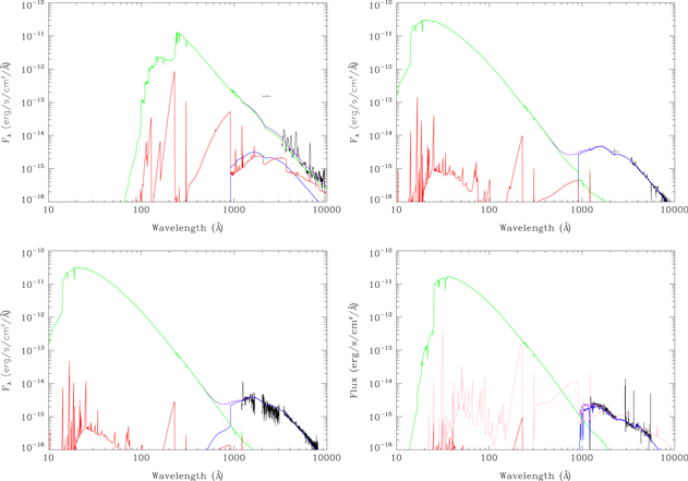
Figure 18. Components of the best fit Cloudy models to the D7.5 (a), D29.5 (b), D42 (c), and D57 (d) rebinned UV and optical spectra, top left to bottom right. Similar to the estimated field star value, the Cloudy models have been reddened by the mean LMC E(B−V) of 0.15 mag (Dutra et al. 2001). The model parameters are given in Table 6. The green line shows the WD contribution, the blue line the secondary source contribution, the red the ejecta contribution, and the purple the summed model. The pluses at 2246 Å in the top two figures show the flux from the uvm2 observation. The ejected shell component is only a significant contributor on the first date when the secondary is not as luminous. The bottom right figure also shows the contribution of a model with the same parameters except for 20X the ejecta mass in pink. It is included to illustrate the amount of mass required to obtain sufficient UV/optical flux similar to the observations. Note that the resulting model UV/optical continuum is a very poor fit to the observed spectra.
Download figure:
Standard image High-resolution imageWe find that the best fit to the continuum from D7.5 which is also consistent with the lack of a Swift detection, used a Rauch model atmosphere with Teff = 130,000 K and a slightly higher bolometric luminosity of 2 × 1038 erg s−1, see Figure 18(a). The implied WD radius from this  and
and  is about 0.1 of the orbital separation, see Section 5. The D7.5 WD parameters and NH = 5 × 1021 cm−2 (for an ejected mass of 10−6
  7 days after the outburst, see below) predict a Swift count rate of 10−8 ct s−1 in PIMMS which is consistent with the observed upper limit of <0.008 ct s−1 on D8.2. The uvm2 magnitude on the same day was converted to a flux (Poole et al. 2008) and is also shown in Figure 18(a). The WD model predicts less continuum flux than is detected at the effective wavelength of the uvm2 filter. The likely explanation for this discrepancy is that the early NUV SED had significant line emission, as seen in the D7.5 optical spectrum, that is not reproduced by the WD model continuum.
At these model temperatures and luminosities, the WD contributes nothing to the observed UV/optical SED except for the first date when the effective temperature was much lower. Figure 18 shows the WD contribution in green and the ejecta contribution in red. Since the WD fits the optical spectra during the first modeled epoch, a strong upper limit on the model ejected mass can be established. A model with an ejected mass Mej = 1.4 × 10⁻⁶  provides the best fit to the data and was adopted for the other three dates. This mass estimate is also consistent with those derived in Section 3.1.2.
The Cloudy fits for the latter three dates were extremely poor, independent of realistic ejecta masses. The predicted continuum was generally at least 100 times lower than the observed SED when using the mass derived from the first modeled epoch. Artificially raising the model ejected mass to significantly larger values did increase the predicted UV/optical continuum luminosity but the resulting recombination spectrum was completely incompatible with the observed SED. Figure 18(d) shows an example the poor fit of a model where the mass was increased by a factor of 20 to match the UV and optical spectra (pink line).
Since the contribution of the model ejecta could not fit the later observations, another light source with peak flux in the UV was required. Building on the assumption that the UV/optical/NIR modulation described in Section 4.1 was due to an illuminated secondary star, we add this contribution to the model. Estimates of the effective temperature of the secondary’s “day” side can be made from geometric arguments of the amount of flux intercepted (Exter et al. 2005) assuming that the secondary is in thermal equilibrium. Rappaport et al. (1982) find that for conservative mass transfer the mass ratio, q = Msec/Mpri, is  To illustrate the expected illumination temperatures under reasonable assumptions consistent with the data, we adopt q = 2/3, a WD mass near the Chandrasekhar limit, and a 19.24 hr period to derive a secondary day-side temperature of 22,000 K. This temperature in a blackbody or model atmosphere was used as the starting point when fitting the UV and optical spectra in the last three observations. The secondary SED contributions are shown in blue in Figure 18.
The best fits to the UV/optical data on D42 require a secondary blackbody with this effective temperature and a luminosity of 5.9 × 1035 erg s−1. A blackbody was used due to the lack of a Balmer discontinuity in the optical data. In the D57 data the Balmer discontinuity was present in the HST data and thus a cooler Kurucz (1979) model atmosphere with  of 17,000 K and
  = 2.5 × 1035 erg s−1 was used. Based on the uvm2 photometry of Figure 3, the field star contamination during the second HST visit was twice as large as in the first HST observation. The Balmer jump is likely from the field star as it contributed about 0.67 times the optical flux at this time.
The D42 blackbody temperature was used for the secondary in the D29.5 fit but with a higher luminosity of 7.4 × 1035 erg s−1. For the D7.5 model, a temperature of 20,000 K and luminosity of 4.7 × 1035 erg s−1 was used, which does not affect the fit from the brighter WD primary, see Figure 18(a).
The derived upper limit on the ejected mass is extremely small but is consistent with the very early X-ray turn-on and turn-off times. The high WD photoionization rate with an extreme effective temperature and bolometric luminosity on a very low mass–shell produces highly ionized ejecta. The typical nebular lines were not observed in LMC 2012 because ions such as O iii, C iv, N ii, and Fe vii are simply not present. The only emission lines that were observed during the nebular phase, N v and possibly (Ne v) and (Fe x), were from high ionization potential species. Without a large number of emission lines, the Cloudy models cannot constrain the ejecta abundances and thus the composition of the WD could not be derived. The final Cloudy model parameters are provided in Table 6.
Table 6. Cloudy Model Parameters
| Value | ||||
|---|---|---|---|---|
| Parameter | D7.5 | D29.5 | D42 | D57 |
WD  |
130 kK | 963 kK | 963 kK | 638 kK |
| WD SED | Rauch log(g) = 8 | Rauch log(g) = 8 | Rauch log(g) = 8 | Rauch log(g) = 8 |
WD  |
2.0 × 1038 erg s−1 | 1.0 × 1038 erg s−1 | 1.0 × 1038 erg s−1 | 7.8 × 1037 erg s−1 |
2nd  |
20 kK | 22 kK | 22 kK | 17 kK |
| 2nd SED | Blackbody | Blackbody | Blackbody | ATLAS log(g) = 4a |
2nd  |
4.7 × 1035 erg s−1 | 7.4 × 1035 erg s−1 | 5.9 × 1035 erg s−1 | 2.5 × 1035 erg s−1 |
| Initial H density | 3 × 109 cm−3 | 2.5 × 107 cm−3 | 2.0 × 107 cm−3 | 6.3 × 106 cm−3 |
| Ri | 6.5 × 1013 cm | 2.5 × 1014 cm | 3.6 × 1014 cm | 5.2 × 1014 cm |
| Ro | 3.2 × 1014 cm | 1.3 × 1015 cm | 1.8 × 1015 cm | 2.6 × 1015 cm |
| Mejectedb | 1.4 × 10⁻⁶  |
1.4 × 10⁻⁶  |
1.4 × 10⁻⁶  |
1.4 × 10⁻⁶  |
Notes. The other Cloudy parameters are a hydrogen density power law of r−3, filling factor of 0.3, covering factor of unity. All abundances were kept at their solar abundances (Asplund et al. 2005, p.25).
a(Kurucz 1979) model atmosphere. bUpper limit.Download table as: ASCIITypeset image
5. DISCUSSION
The available LMC 2012 data provide insight into the nature of the binary system. The rapid optical decline, early SSS detection, very short SSS duration, bright SSS luminosity, high WD effective temperature, large ejection velocities, and low estimated ejected mass are all consistent with a high mass WD, likely near the Chandrasekhar limit.
WD mass estimates can be found from various relationships established in the literature. The models of Sala & Hernanz (2005) show that for a WD with k  keV and L = 1 × 10⁵
  the mass must equal or exceed 1.3
  regardless of assumed WD plus accretion composition mix. Likewise, the Yaron et al. (2005) models that best match the observational parameters for LMC 2012 have a WD mass between 1.25 and 1.4
  with an accretion rate about 1 × 10⁷–8
  yr−1. An additional mass estimate can be obtained from the more recent WD modeling of Wolf et al. (2013). For LMC 2012, the turn-off time (∼50 days) and maximum effective temperature imply a WD mass between 1.30 and 1.34
  . It should be noted that all of these models do not take into account all the parameters that are likely to have a role amount of mass accreted and ejected so the WD mass derived from the LMC 2012 values is only approximate. Regardless, the available models are all consistent with a WD mass above 1.3
  .
.
The observed modulation of 19.24 hr in the uvm2, BVRI and JHK light curves from D20 to D60 is most likely associated with the orbital period. All the data presented in this analysis are best explained by the illumination of the secondary day-side to effective temperatures of order 22,000 K by the hot WD primary in a relatively high inclination system.
Some limits on the inclination of the system can be established from the available spectra. The inclination has to be much less than 90 since eclipses are not seen in either the X-ray or UV data. The inclination from the line profile analysis, 70
 is consistent with the absorption spectrum observed in the high resolution Chandra grating spectrum. Ness et al. (2013) find that the type of X-ray spectrum, absorption or emission, is determined by the system geometry. Emission line X-ray spectra are associated with high inclination systems because the lines are from reprocessed emission in the accretion disk.
Assuming q = 2/3, a Chandrasekhar mass WD, and a 19.24 hour orbital period, the system separation is 3.2 × 1011 cm  and the secondary Roche lobe radius is 1.0 × 1011 cm
  In order to achieve mass transfer, the secondary must have a radius equal to its Roche lobe radius which implies a subgiant. The inferred temperature from the UV and optical continuum fit is much higher than expected for a late type subgiant. However the day-side temperature in irradiated models can reach factors of between four and ten times larger than the shadowed side (e.g., Wawrzyn et al. 2009).
A late type subgiant secondary at quiescence would be > 4 mag fainter than the nearby field star and thus not observed in pre-outburst surveys. The outburst amplitude would be >10 mag which is also consistent with the very fast t2 time.
The mass accretion rate can be estimated assuming the mass loss rate of an evolved secondary filling its Roche lobe and including magnetic stellar winds (see Equations (3.16)–(3.20) in Iben & Fujimoto 2008). The mass accretion rate is 10−8  yr−1 using the same assumptions as before, namely a Chandrasekhar mass WD, q = 2/3, and Porb = 19.24 hr. Table 1 in Gehrz et al. (1998) provides the WD envelope mass necessary to reach the critical pressure to initiate a TNR as a function of WD mass. At the upper end, MWD = 1.35
  , the envelope mass is 4 × 10⁻⁶
  . For the estimated mass accretion rate, the time to obtain this envelope mass is very short, 60 years. This gives further credibility to the hypothesis that LMC 2012 is a recurrent nova of the U Sco subclass. It is unlikely that archival searches of the LMC would turn up any previous events as the 2012 outburst was only brighter than 16th mag in the V band for about a week.
Maintaining a 105  bolometric luminosity for 50 days requires 1.4 × 10⁻⁷
  of hydrogen to remain on the WD after the initial explosion (Gehrz et al. 1998). This amount is 20% of the estimated upper limit on the ejected mass. The ejected mass plus the WD mass burned is still about four times less than the accreted mass for a 1.35
  WD and suggests that the WD is growing in mass. This makes LMC 2012 a potential SN Ia progenitor (Starrfield et al. 1988; Woodward & Starrfield 2011; Starrfield 2014) assuming the WD is not of the ONe class (e.g., Mason 2011). Unfortunately the lack of many shell emission lines makes an abundance determination from the available data problematic.
6. SUMMARY
- 1.LMC 2012 had a very fast optical/UV decline and its optical spectral evolution was similar to that of U Sco. The V band t2 time of two days was one of the fastest ever observed. Detection of similar outbursts in the LMC will require full time monitoring at a high cadence since this nova was brighter than V = 16 mag for less than 8 days. The telescopes and detectors of most amateur astronomers are only sensitive to visual magnitudes brighter than about 13 mag.
- 2.An expansion velocity of ∼5000 km s−1 was inferred from P-Cygni absorption observed in the early optical spectra. Absorption lines with similar blue shifts were also observed in the later Chandra SSS spectrum.
- 3.LMC 2012 evolved very rapidly in the X-ray band with turn-on and turn-off times of ∼13 and 50 days, respectively. Both X-ray timescales are extremely short compared to most other Galactic (Schwarz et al. 2011) and M31 novae (Henze et al. 2014). To model the X-ray evolution we fit all the Swift observations with a series of Rauch (2003) model atmospheres. We confirmed this approach by sucessfully fitting the single Chandra observation with a model atmosphere with similar parameters as determined from the Swift data set around the same time. The results reveal a very hot WD with maximum effective temperatures of 86.2 ± 0.3 eV, ∼1 MK, during the SSS phase. This temperature is also one of the highest ever found in a nova and similar to that of RS Oph (Osborne et al. 2011) and V745 Sco (Osborne et al. 2014). The X-ray luminosity from the model atmosphere fits was constant from D20 to D50 at ∼1 × 1038 erg s−1.
- 4.The UV, optical and NIR light curves all showed oscillatory behavior during the X-ray SSS phase. Using the Swift uvm2 data, we find a period of 19.24 hr. The BVRI and JHK data sets can also be well fit with the same period. There is no similar periodicity in the X-ray light curve. The period derived from the UV–IR modulation is likely orbital in nature. The line profile fitting of the Hα line provides an inclination estimate of 60 ± 10
 which is consistent with both the modulation amplitudes observed in the various filters and the strong absorption lines detected in the Chandra grating observation (Ness et al. 2013).
 - 5.An extremely unusual discovery was that the UV spectra only showed the N v line at 1240 Å. Even in the optical, the emission lines quickly faded as the nova progressed to the SSS phase showing no nebular lines and weak, if any, coronal lines. The puzzling lack of lines can be explained by the high ionization of the low mass ejecta which was largely ionized by a hot and luminous WD. The very low upper limit on the hard X-ray, >1 keV, luminosity is also consistent with a small ejection mass since there is less material to be involved in shock emission.
- 6.All the observed UV and optical continuum data can be fit with a binary system model consisting of a hot WD, whose photoionization parameters are derived from the fits to the X-ray data set, ionizing a very small amount of ejected material (∼1 × 10⁻⁶) and illuminating a secondary source. The extremely small derived ejecta mass contributes essentially nothing to the later observed spectral energy distribution. The contribution from the secondary is primarily responsible for the later UV/optical SEDs whereas the earliest optical spectra are consistent with the Rayleigh–Jeans tail of a WD photosphere too cool at that time to be detectable in X-rays.
- 7.The rapid X-ray, UV, and optical evolution, the large expansion velocities seen throughout the outburst, plus the low mass ejected imply LMC 2012 is a recurrent nova of the U Sco subclass occurring on a high mass WD in a moderately long period system with a high mass accretion rate. The available evidence implies that the WD is gaining mass every outburst. Unfortunately, the lack of significant line emission in the UV and optical spectra did not allow us to determine the ejecta abundances and thus the WD composition could not be inferred. Future modeling of the Chandra spectrum may provide the necessary insights on the WD composition.


This research has made use of data obtained from NASA’s Swift satellite. We thank Neil Gehrels and the Swift team for generous allotments of ToO and fill-in time. We thank Harvey Tananbaum for the Chandra Director’s Discretionary Time observation of LMC 2012. Support for HST Program number 12484 was provided by NASA through a grant from the Space Telescope Science Institute, which is operated by the Association of Universities for Research in Astronomy, Incorporated, under NASA contract NAS5-26555. Stony Brook University’s initial participation in the SMARTS consortium was made possible by generous contributions from the Provost of Stony Brook University. We acknowledge with thanks the variable star observations from the AAVSO International Database contributed by observers worldwide and used in this research. KLP, JPO & APB acknowledge the support of the UK Space Agency. S.S. acknowledges partial support from NASA and NSF grants to ASU. This research has been supported in part at the University of Chicago by the National Science Foundation under Grant PHY 08-22648 for the Physics Frontier Center “Joint Institute for Nuclear Astrophysics” (JINA). Finally, we thank the referee for a thoughtful report that greatly improved the paper.
Facilities: HST(STIS) - Hubble Space Telescope satellite, Swift(XRT and UVOT) - Swift Gamma-Ray Burst Mission, AAVSO - American Association of Variable Star Observers International Database, CTIO:1.3m - , CTIO:1.5m - , CXO - Chandra X-ray Observatory satellite
Footnotes
- *
Based on observations with the NASA/ESA Hubble Space Telescope obtained at the Space Telescope Science Institute, which is operated by the Association of Universities for Research in Astronomy, Incorporated, under NASA contract NAS5-26555.
- 11
- 12
- 13
- 14
Grid #011 from http://astro.uni-tuebingen.de/∼rauch/TMAF/flux_HHeCNONeMgSiS_gen.html In the framework of the Virtual Observatory (VO; http://www.ivoa.net), these spectral energy distributions are available in VO compliant form via the VO service TheoSSA (http://vo.ari.uni-heidelberg.de/ssatr-0.01/TrSpectra.jsp?) provided by the German Astrophysical Virtual Observatory (GAVO; http://www.g-vo.org).