Abstract
Most large galaxies harbor supermassive black holes (SMBHs) in their centers, and galaxies merge. Consequently, binary SMBHs should be common in galactic nuclei. However, close binaries of SMBH (CB-SMBHs) with subparsec separation cannot be imaged directly using current facilities. Some indirect signatures, such as periodic signals in light curves and double peaks in the emission-line profile, have been used to find CB-SMBH candidates, but ambiguities still exist and no definitive conclusions can be made. We have recently proposed a new method focusing on kinematic signatures that can be derived from reverberation mapping of CB-SMBHs, one that offers a promising avenue to address this important problem. In this paper, we calculated models for a wide range of parameters, but broad-line regions of two BHs are close but still not merged. The purpose of this supplementary paper is to provide an atlas of two-dimensional transfer functions of CB-SMBHs with a wide range of orbital and geometrical parameters to aid more efficient identification of CB-SMBH candidates in reverberation mapping data.
1. Introduction
The existence of supermassive black holes (SMBHs) at the center of active galaxies was first proposed to explain the ultimate energy source of quasars (Salpeter 1964; Zel’dovich 1964; Lynden-Bell 1969). Most galaxies are believed to host quiescent SMBHs, remnants of their earlier active phases (Begelman et al. 1980). This has since been confirmed from dynamical observations of the stars and gas in the Milky Way (Schödel et al. 2002) and nearby galaxies (Kormendy & Ho 2013). Mergers between galaxies are predicted by hierarchical structure formation (Lacey & Cole 1993) in the standard cosmological model, and they have been studied statistically in numerous surveys (Patton et al. 2002; Lin et al. 2004; Conselice 2014). Binary SMBHs settling in the cores of merged galaxies are thus expected to be quite common, with separations and orbits that depend on their stage of evolution (Begelman et al. 1980).
A number of SMBH binaries with kiloparsec-scale separations have already been found (Komossa 2003; Bianchi et al. 2008; Comerford et al. 2009, 2013, 2015; Wang et al. 2009; Green et al. 2010; Koss et al. 2011; Liu et al. 2011, 2018; Fu et al. 2015). To date, the closest SMBH pair that has been spatially resolved has a projected separation of 7.3 pc (Rodriguez et al. 2006). Close binaries of SMBHs (CB-SMBHs) with subparsec separation are hard to image directly with existing facilities. Alternative indirect methods are needed to confirm their existence observationally.
Periodicity is one of the most distinguishing features of a binary system (e.g., MacFadyen & Milosavljević 2008; Roedig & Sesana 2014; Farris et al. 2015; Shi & Krolik 2015; Bowen et al. 2018). Periodic signals possibly due to the modulation of orbital motions of SMBH binaries have been found in the light curves of a handful of objects, including OJ 287 (Sillanpaa et al. 1988), PG 1302−102 (Graham et al. 2015), SDSS J0159+0105 (Zheng et al. 2016), NGC 5548 (Li et al. 2016), and Ark 120 (Li et al. 2019).6 For a secure identification of the periodicity with orbital motion, the monitoring duration should be at least three times the period (Li & Wang 2018). The period of a typical CB-SMBH is

where M8 = Mtot/108M☉ is the total mass of the system, and A30 = A/30 light days (lt-day) is the separation between two BHs. Given the limited time span of the existing monitoring data for most active galactic nuclei (AGNs), only binaries with separations around several light days can be detected in this way. The interaction between the accretion disks (Hayasaki et al. 2008) and effects of general relativity (D’Orazio et al. 2015) must be considered, making the theoretical interpretation and confirmation nontrivial.
Another important feature of CB-SMBHs is the relative velocity between the two BHs, which is about

When the inclination along the line of sight (LOS) and the phase of the rotation are taken into account, the relative velocity is sufficiently significant to leave an imprint on the profiles of emission lines, such as double-peaked and asymmetric signatures (Popovic et al. 2000; Shen & Loeb 2010; Tsalmantza et al. 2011; Popović 2012). Shift of line center or shape of asymmetry in the single-epoch broad-line profile have been found in objects like SDSS J153636.22+044127.0 (Boroson & Lauer 2009), NGC 4151 (Bon et al. 2012), and NGC 5548 (Li et al. 2016), making them promising CB-SMBH candidates. However, the line profile is highly degenerate in its ability to distinguish the intrinsic dynamics of the gas in the broad-line region (BLR). Complex BLR models can also produce double-peaked or asymmetric broad emission lines (Wang et al. 2017). These features alone cannot prove the existence of CB-SMBHs definitely, and more information is needed to break the degeneracy.
One possible approach is reverberation mapping (RM), which is used to infer the spatial scale of the BLR in time domain (Blandford & McKee 1982; Peterson 1993). Although broad-line profiles in the CB-SMBH and disk emitter cases could be similar, Shen & Loeb (2010) generally argued that they reverberate differently to the continuum variations. We note that velocity-resolved RM data have one more dimension than a line profile, reflecting the velocity distribution of the ionized gas on different spatial scales, and so can be used to probe the gravitational potential around the central BH. Since the gravitational potential around a CB-SMBH is much different than that of a single SMBH, RM data of CB-SMBHs must contain some distinctive kinematic signatures (Wang et al. 2018). Wang et al. (2018) provided semianalytical formulae for two-dimensional (2D) transfer functions (TFs) of emission lines to continuum in typical CB-SMBH models, and several examples were illustrated to show the peculiarities of CB-SMBHs in contrast with single SMBHs. We are conducting a long-term project of Monitoring AGNs with Hβ Asymmetry (MAHA) using the Wyoming Infrared Observatory 2.3 m telescope to hunt for CB-SMBHs in the local universe (Du et al. 2018a; Brotherton et al. 2019). Some indications of CB-SMBHs have been found in the 2D TFs of Mrk 6 and Akn 120, but more data are needed for further confirmation.
We also note that the recently deployed GRAVITY instrument on the Very Large Telescope Interferometer (VLTI) successfully spatially resolves the BLR in 3C 273 through the S-shaped differential phase curve (DPC) of the Paα emission line (Gravity Collaboration et al. 2018). DPCs of binary BLRs do possess distinguishing features compared to those from a single BLR due to the separation of the two BLRs and the orbital velocity of the system. These differences can be exploited to reliably identify CB-SMBHs (Songsheng et al. 2019). RM campaigns can provide not only CB-SMBH candidates for GRAVITY observations, but they also can be analyzed jointly with GRAVITY data to reduce the uncertainties of the orbital parameters and provide directly the cosmic distance to the BH (Wang et al. 2020).
As the MAHA project and other RM campaigns (such as SDSS-RM project described by Shen et al. 2015) move forward, a large sample of AGNs will be available for searching for CB-SMBHs. A direct and efficient method is needed for preliminary selection of CB-SMBH candidates. In this supplementary paper, we calculate a series of atlases of 2D TF for CB-SMBHs with various possible orbital and geometric parameters. Given the continuum and velocity-resolved emission-line light curves from the RM campaign, 2D TFs of BLRs can be reconstructed straightforwardly using the maximum entropy method (MEM; Horne 1994; Xiao et al. 2018a). Presenting complete features of 2D TFs for various CB-SMBH systems, the TFs extracted from current and future RM data can be directly compared against our atlases to select CB-SMBH candidates efficiently. A few targets from the MAHA campaign show promising signatures of CB-SMBHs (in a forthcoming paper). Even rough ranges of orbital parameters are possible to be estimated by direct comparison, which is important for further detailed analysis and confirmation.
2. Reverberations of Binary BLRs
Reverberation mapping is a powerful tool to measure the kinematics of ionized gas around BHs. The technique makes the following assumptions: (1) the origin of the ionizing photons (the accretion disk) is a point source much smaller than the BLR; (2) photoionization is the dominant ionization mechanism for the emission lines; and (3) the BLR is relatively stable within the reverberation mapping timescale (see reviews of Peterson 1993, 2014). A single accreting BH is usually assumed as the default in the galactic center, but obviously this is inappropriate in the case of CB-SMBHs. Composition of reverberations of binary BLRs should be investigated for cases of CB-SMBHs, which are still spatially unresolved for direct imaging.
In the seminal paper of Blandford & McKee (1982), the reverberation of emission lines in response to continuum variations is mathematically described by the convolution

where Lℓ(v, t) and  are the light curves of the emission lines and continuum, respectively, and Ψ(v, t) is the 2D TF, which encodes the geometric and kinematic information of the BLRs. This function presents the echo strength of the emission line (ℓ) in the space of the velocity of the line profile and delays. Observations provide data for the light curves of the velocity bins and ionizing fluxes. From the convolution theorem, it follows

where

where ω is the angular frequency in Fourier space, and  are the Fourier transform and inverse Fourier transform, respectively. We stress that this formal expression does not assume the case of a single SMBH and a single BLR.
The construction of 2D TFs of binary BLRs has been discussed by Wang et al. (2018). For convenience, we extend the derivation briefly here and use simulations to show the validity of the linear approximations. In this stage, we assume that the CB-SMBHs have their own BLRs, each ionized only by its own accretion disk. This assumption should be revised, as described in a forthcoming work, if the binary BLRs have merged to a later phase, in which case the CB-SMBH would be surrounded by a common BLR with an asymmetric geometry that is photoionized by two ionizing sources. The two independently varying continuum sources are denoted as  , and the corresponding broad emission lines are
  . Then, for a spatially unresolved CB-SMBH, the total continuum and line emission are

The linear combination of two independent components can be expressed linearly in Fourier space:

Inserting Equation (7) into (4), the 2D TF is
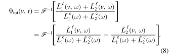
Introducing the individual 2D TFs, we have
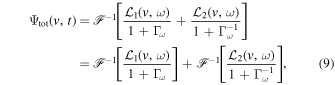
where

and the coupling coefficient is given by  , which is caused by the limitation of spatial resolution of the telescope. The quantity
  cannot be given analytically a priori, but we can derive it from the properties of the optical variability of AGNs with single BHs. This paper provides more discussion on this coupling coefficient.
It should be noted that ![${{\rm{\Psi }}}_{\mathrm{1,2}}(v,t)={{\mathscr{F}}}^{-1}[{{ \mathcal L }}_{\mathrm{1,2}}(v,\omega )]$](https://content.cld.iop.org/journals/0067-0049/247/1/3/revision1/apjsab665aieqn7.gif) , where Ψ1,2(v, t) are the single TFs of the two BLRs. Using the convolution theorem again, we have
, where Ψ1,2(v, t) are the single TFs of the two BLRs. Using the convolution theorem again, we have

where

The sum of  and
and  is
is

If  is a real constant Γ0, we find that
  and
and  , and so

That is, the total TF is a linear combination of two individual TFs. However, Γω generally is not a constant. Given each BLR and the coupling coefficient, we can specify the composite 2D TF.
3. The Coupling Coefficient
3.1. Generating Light Curves
A number of monitoring campaigns have shown that AGN brightness varies as a continuous stochastic process, which can be described by the power spectral density (PSD) of its variation. Earlier optical observations find that the PSD of quasars is a single power law with index γ ≈ 2 (Giveon et al. 1999), consistent with a damped random walk (DRW, Li et al. 2013; Zu et al. 2013). However, there is growing evidence for deviations from the DRW model, with  in 13 AGNs (Collier & Peterson 2001), γ = 1.77 in MACHOS quasars (Hawkins 2007), and γ = 1.75 − 3.2 in Kepler quasars (Smith et al. 2018). For the present discussion, we generalize the PSD in the form

where τ0 is the characteristic timescale of variations, σ is its amplitude, γ is the power-law index, and cγ is a normalization constant. There are two regimes of interest: (1) when  , PSD is a constant; (2) when
  ,
,  . The present PSD functions fulfill the conditions of most observations, and hence satisfy the requirements for
  .
.
As shown by Timmer & Koenig (1995), the PSD of variations is the Fourier transform of its auto-covariance function (ACF). That is,

where  is the deviation of the AGN’s magnitude from its expectation value at time t. In practice, cγ can be obtained from

As a natural consequence, we have  in our formulation. Given the PSD of the variations, realization of the process (i.e., light curve of the AGN) can be simulated by the algorithm, which is easy to implement (Timmer & Koenig 1995). The major steps are as follows: (1) for each angular frequency ω, draw a random number from a chi-squared distribution with 2 degrees of freedom, then multiply it by PSD(f = ω/2π)/2. This will be used as the module of the variation in Fourier space
  . (2) The phase angle of
  is generated uniformly between 0 and 2π. (3) The inverse Fourier transform of
  yields ΔM(t), and M(t) is given by
  . (4) The magnitude M(t) now can be converted directly to luminosity L(t). This scheme allows us to test the properties of the coupling coefficient (
 ).
).
3.2.
 -dependence

In order to test the  -dependence, we use correlations of τ0 and σ with optical luminosity from Kelly et al. (2009), who analyzed a sample of AGN optical light curves and modeled them as a stochastic process with γ = 2. Given the 5100 Å luminosity, τ0 and σ are found from the intermediate correlations with AGN luminosity, which are given by

Here the σ correlation is converted from Kelly et al. (2009), as their definition of σ is different from ours. Although the above relations assume γ = 2, we will utilize them in our simulations to generate light curves for  . Examples of simulated continuum light curves and the corresponding
  are illustrated in Figure 1.
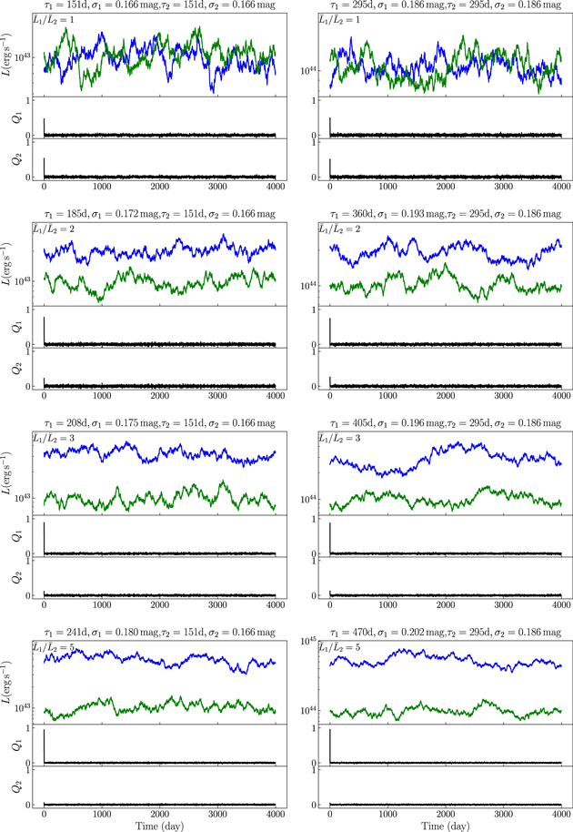
Figure 1. Examples of simulated continuum light curves and corresponding  functions. In the left panels, the average L5100 of the secondary BHs are all
  , and the luminosity ratios are 1, 1/2, 1/3, and 1/5 from top to bottom. In the right panels, the average L5100 of the secondary BHs are all
  , and the luminosity ratios are also 1, 1/2, 1/3, and 1/5 from top to bottom. The timescales and amplitudes of variations are obtained through Equation (17).
Download figure:
Standard image High-resolution imageFor a wide range of average luminosity and luminosity ratios, our simulation shows that  for the primary BH can always be treated as delta functions with minor noise. If we assume
  , we immediately will obtain
  from Equation (12). Thus, the total transfer function can be calculated as

The coefficient q1 is correlated with the luminosity ratio in our simulations, as shown in Figure 2.
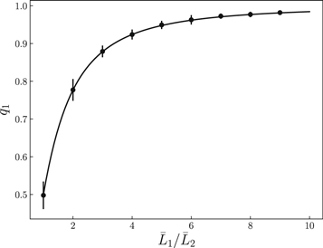
Figure 2. Correlation between the coefficient of linear combinations and luminosity ratios. The average L5100 of the secondary BH is taken to be  . The timescales and amplitudes of variations are obtained through Equation (17). For every data point, 100 light curves are generated to calculate the value and uncertainty for the coefficient q1. We also note that the correlation can be well described by an empirical formula,
 ![${q}_{1}=1-1/[{({\bar{L}}_{1}/{\bar{L}}_{2})}^{1.8}+1]$](https://content.cld.iop.org/journals/0067-0049/247/1/3/revision1/apjsab665aieqn36.gif) (solid line).
(solid line).
Download figure:
Standard image High-resolution imageNevertheless, we should mention that the noise amplitude of  depends on the cadence and duration of the sampling. Only if the cadence is much shorter than the timescale of the variation of both continuum sources while the duration is much longer will our linear approximation be valid. This is reasonable since it is almost impossible to extract TF from poor RM data with bad cadence and short duration, even in the case of a single BLR.
4. BLR Models and Transfer Functions
4.1. Kinematics
Much progress has been made in reverberation mapping campaigns during the last three decades, particularly in the application of the velocity-resolved technique to study the kinematics of the BLR. There is growing evidence that the BLRs in most AGNs have rather simple geometry and dynamics. Flattened disks are common in Seyfert galaxies (Grier et al. 2013), even among narrow-line Seyfert 1 galaxies (Du et al. 2016). Inflows or outflows have been reported in a few cases. Detailed investigations of a few objects (e.g., NGC 5548, 3C 390.3, and NGC 7469; Wandel et al. 1999; Lu et al. 2016) show that the FWHM of Hβ and its lag follows  , indicating a Keplerian rotating disk. This conclusion is supported by detailed dynamical modeling (Pancoast et al. 2011, 2014a, 2014b; Li et al. 2013, 2018; Grier et al. 2017). This paper only focuses on models in which the binary BLRs are still independent so that each BLR can be described by a flattened disks. We do not exclude the presence of inflows or outflows, but here we are mainly concerned with the disk-like geometry of the BLRs.
Table 1 lists the parameters of the present model. For each BLR, the main parameters are the inner and outer radii ( and
and  ), the power-law index of the reprocessing coefficient (γi for the two BLRs), and the half-opening angle (Θi). The binary BLRs are rotating around the center of mass of the binary BHs, and the binary disks are aligned with the orbital plane. Each flattened BLR is allowed to rotate in the same or completely opposite direction as the orbital motion. In future, polarized spectra or DPCs obtained by GRAVITY (Songsheng et al. 2019) may be able to resolve the sense of rotation, but this effect cannot be distinguished in the total spectra.
Table 1. Parameters of the Binary BLR Model
| Parameters | Description | |
|---|---|---|
| A | Separation between two BHs | |
| T | Rotation period of the binary system | |
| For the binary | μ1 | Mass fraction of the primary BH |
| i | Inclination angle of the LOSa | |
| ϕ | Phase angle of the rotation relative to the LOSb | |
| Γ0 | Coefficients of the linear combination in Equation (18) | |
| Rin | Inner radius of the BLR | |
| Rout | Outer radius of the BLR | |
| For individualsc | Θ | Opening angle of the BLR |
| γ | Power-law index of reprocessing coefficient distribution | |
| α0(β0) | Velocityd of inflow (outflow) at outer radius | |
| α(β) | Power-law index of inflow (outflow) velocity | |
Notes.
ai = 0° indicates face-on orientation. bϕ = 0° indicates that the connection between two BHs is perpendicular to the LOS. cThere are two sets of these parameters; subscripts are eliminated here. dIn units of local Keplerian velocity.Download table as: ASCIITypeset image
Given the velocity field and the reprocessing coefficient distribution of each BLR, the 2D TF in principle can be calculated according to Blandford & McKee (1982). Suppose that the velocity distribution of the clouds in BLR i at a given point is  , where
  is the displacement to its central BH and
  is the velocity of the cloud. The reprocessing coefficient at that point is
  . The 2D TF for the BLR is therefore

where  is the unit vector pointing from the observer to the source. However, the orbital motion should be included in the velocity field of each individual BLR. It should be noted that the composite velocities of clouds is the superposition of the individual virial motion (or inflow/outflow motion) and orbital motion of the binary system. Thus,
  , where
  is the angular velocity of the system,
  is the displacement of the central BH from the center of mass of the system, and
  is the virial velocity of the cloud in the corotating frame. As the rotation period of the system (tens or hundreds of years) is much longer than the timescale of reverberation (tens or hundreds of days),
  ,
,  , and
, and  are considered to be invariant when calculating the TFs.
4.2. Atlas of 2D TFs
This paper focuses on the separated binary BLRs of CB-SMBHs. The individual BLR is assumed to follow the scaling relation between size and optical luminosity as  lt-day, where
  (Bentz et al. 2013). It should be noted that this only applies to sub-Eddington AGNs (Du et al. 2014, 2015, 2018b). Given the BH mass, the optical luminosity at 5100 Å can be calculated by

where λ0.01 = λEdd/0.01 is the Eddington ratio and κ10 = κbol/10 is the bolometric correction factor. The average radius of the BLR can be expressed as

The average radius of BLR is defined by

where  is the reprocessing coefficient. Given the separation between the two BHs and the rotation period of the binary system, the Keplerian relation can be expressed by Equation (1). We choose the BH mass from 106 to 1010 M☉. Since we assume that the CB-SMBHs have their own BLRs and each ionized only by its own accretion disk, the two BLRs must be well separated. Thus, there is another additional constraint on the separation,

which limits the space of the CB-SMBH parameters. In our calculations, we will assume  and κ10 = 1 for both BLRs. The inner and outer radii of the BLRs will then be taken as
  and
and  , corresponding to γ = 0.5 and Rout/Rin = 3. The masses of the primary and secondary BH can be obtained through M1 = μ1Mtot and M2 = (1 − μ1)Mtot, where μ1 is the mass ratio of the primary BH with respect to the total mass. Figure 3 shows the allowed region in the A–T plane. In this paper, we only consider the cases with μ1 ≤ 0.9. Systems with μ1 > 0.9 may have very different kinematics, and will be treated in a forthcoming paper.
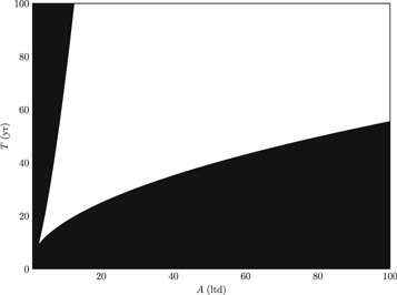
Figure 3. Allowed region in the A–T plane when μ1 = 0.7. Only parameters in the white region are valid. Ranges of allowed regions for different μ1 are very similar. The rotation period for binary BLRs before merging is mostly larger than 20 yr.
Download figure:
Standard image High-resolution imageThe opening angle of the flattened Keplerian disk and the inflows/outflows will be fixed at 10° and 45°, respectively. In the case of inflows, the velocity of the gas at  is assumed to be
  , which is slightly smaller than the local escape velocity. For outflows, the velocity is
  , slightly higher than the local escape velocity, such that the gas gains energy steadily when escaping outward.
In simulations of continuum light curves and  shown in Figure 1, we find that the coefficient Γ0 in linear combinations of individual TFs is generally correlated with the ratio of the average optical luminosity of the two BHs. We also assume that the optical luminosity is proportional to the mass of the BH. As a crude simplification, the total TF will be obtained from the individual TFs through

We have five free parameters to vary when making the atlas of 2D TFs for binary BLRs. The separation A and period T must lie within the white area of Figure 3: we take (A, T) = (10 lt-day, 20 yr), (10 lt-day, 50 yr), (20 lt-day, 50 yr), (20 lt-day, 100 yr), (50 lt-day, 50 yr), (50 lt-day, 100 yr), and (100 lt-day, 100 yr). For each pair of (A, T), the mass fraction of the primary BH will take values of μ1 = 0.6, 0.7, and 0.8, the inclination angle along the LOS will pass through i = 15°, 30°, and 45°, and the phase angle of the rotation will assume values of ϕ = 0°, 45°, 90°, 135°, and 180° to cover half a rotation period.
The atlases of 2D TFs are shown in the following pages. The TF of a binary BLR consisting of two thin disks is composed of two shift bells. The height of each bell is mainly determined by the size of the BLR, while the width of the bell reflects the maximum velocity of clouds along the LOS, determined by the mass of its BH, the size of BLR and inclination of LOS. The separation between the two bells is governed by the orbital velocity of the binary BHs along the LOS, determined by the distance between two BHs, orbital period, orbital phase, and inclination.
From Figure 4, it can be seen that when the phase angle increases from 0° to 180° the two bells of the TF approach each other in the beginning, and then separate and move to the opposite side. When the inclination increases, the width and separation of the bells will become larger owing to the increase of projected velocity. The edge of the bell also becomes sharper when the BLRs are viewed edge-on. The mass ratio of the primary BH adjusts the relative size of the two bell shapes in the TF. When μ1 ≳ 0.8, the effect of the secondary BLR will be hard to detect if we assume that the Eddington ratios of two BHs are comparable. The 2D TFs of two disk-like BLRs with other combinations of (A, T) are shown in Figures 5–10. Their shapes and dependence on inclination, orbital phase, and mass ratio are similar to the case in Figure 4. Only the scales of time and velocity are different.
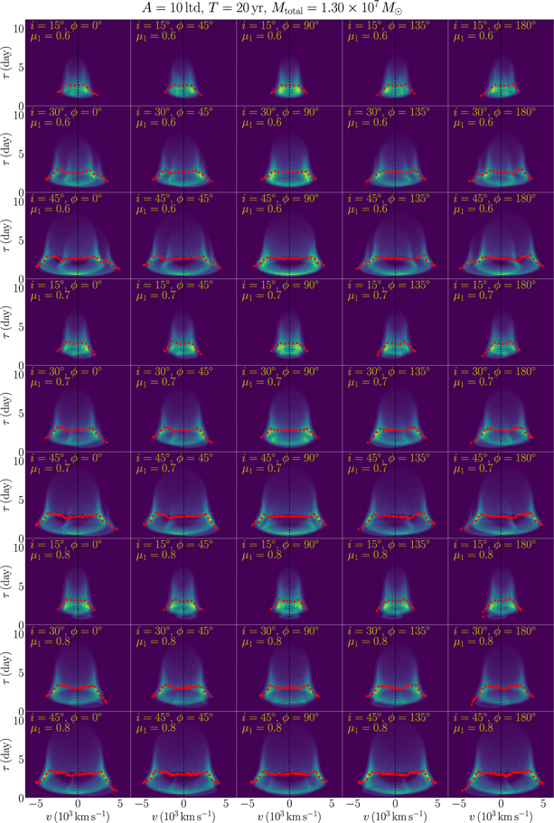
Figure 4. Atlas of 2D TFs of two disk-like BLRs with A = 10 lt-day and T = 20 yr.
Download figure:
Standard image High-resolution image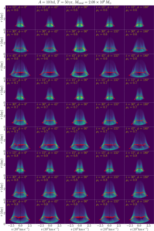
Figure 5. Atlas of 2D TFs of two disk-like BLRs with A = 10 lt-day and T = 50 yr.
Download figure:
Standard image High-resolution image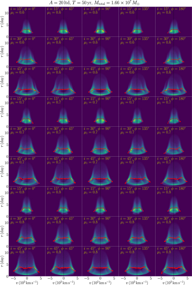
Figure 6. Atlas of 2D TFs of two disk-like BLRs with A = 20 lt-day and T = 50 yr.
Download figure:
Standard image High-resolution image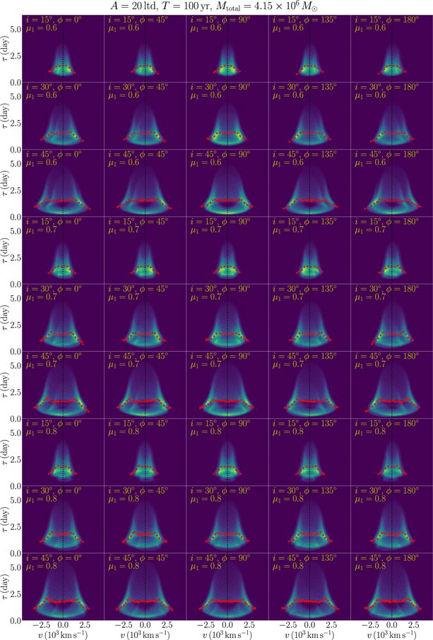
Figure 7. Atlas of 2D TFs of two disk-like BLRs with A = 20 lt-day and T = 100 yr.
Download figure:
Standard image High-resolution image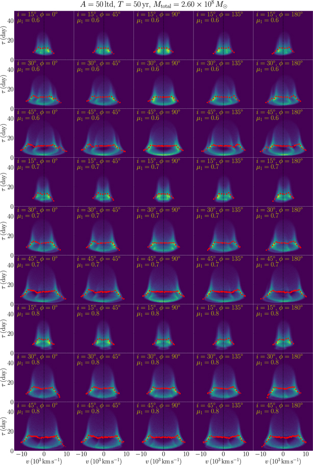
Figure 8. Atlas of 2D TFs of two disk-like BLRs with A = 50 lt-day and T = 50 yr.
Download figure:
Standard image High-resolution image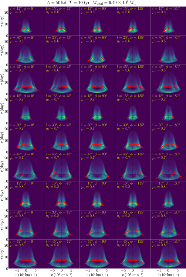
Figure 9. Atlas of 2D TFs of two disk-like BLRs with A = 50 lt-day and T = 100 yr.
Download figure:
Standard image High-resolution image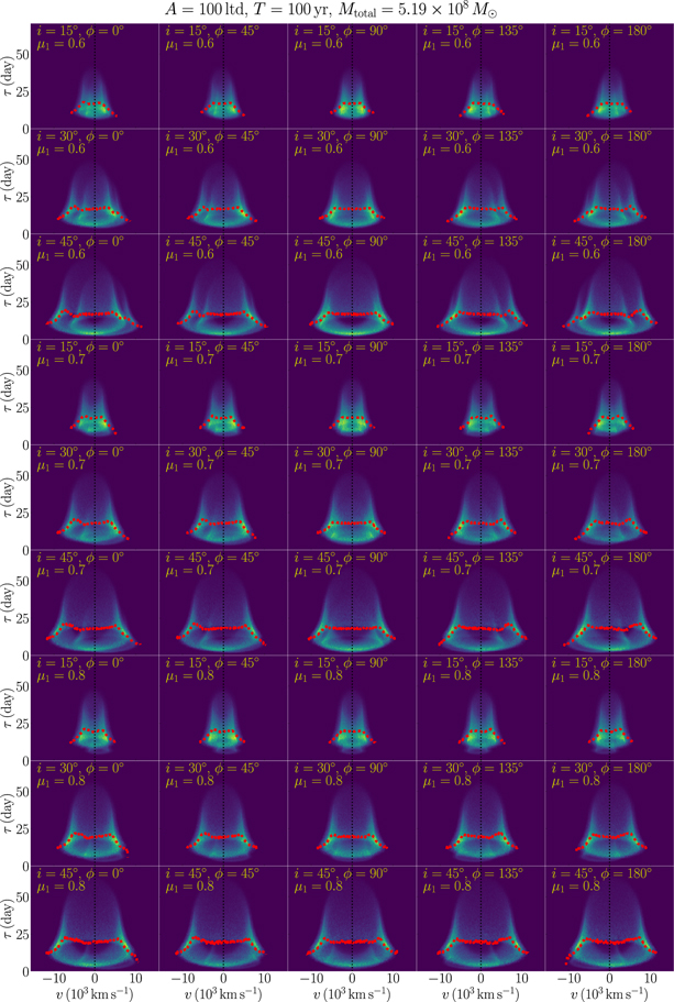
Figure 10. Atlas of 2D TFs of two disk-like BLRs with A = 100 lt-day and T = 100 yr.
Download figure:
Standard image High-resolution imageFigure 11 shows the atlas of 2D TFs for a disk-like BLR plus an inflowing BLR. We only present the case with A = 10 lt-day and T = 20 yr, since the separation and period only affect the scale of the TFs. Each 2D TF is a superposition of a bell shape and a fan shape. The fan shape is inclined so that the delay distribution on the blue side is large and wide, while the delay on the red side is small and narrow. The impact of inclination, orbital phase, and mass ratio are similar to the case of two disk-like BLRs. We also note that the velocity-binned time lags show distinctive features when compared to those of a single disk-like BLR. The blue side of the lags usually shows an extra peak instead of decreasing, while the red side drops to zero.
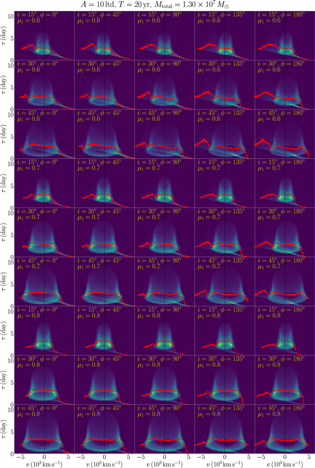
Figure 11. Atlas of 2D TFs of one disk-like BLR and one inflowing BLR with A = 10 lt-day and T = 20 yr.
Download figure:
Standard image High-resolution imageLastly, the atlas of 2D TFs for a disk-like BLR in combination with an outflowing BLR is shown in Figure 12. They are similar to those in Figure 11, except that the fan shape is reflected about the zero velocity line.
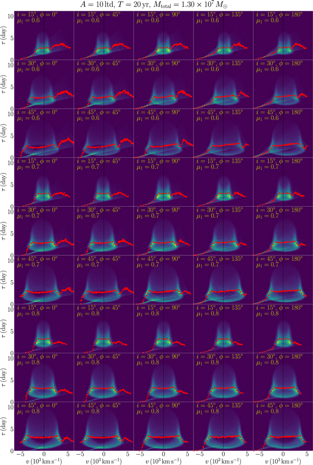
Figure 12. Atlas of 2D TFs of one disk-like BLR and one outflowing BLR with A = 10 lt-day and T = 20 yr.
Download figure:
Standard image High-resolution image5. Discussion
We have presented a formulism for calculating the 2D TFs of binary BLRs and calculated the TFs using a simple but generic model, with a wide range of model parameters. The results are shown as a series of atlases of 2D TFs. Given observed TFs from RM campaigns, we can directly compare them with the atlases presented here to select candidate CB-SMBHs and roughly infer the geometry and kinematics of the constituent BLRs. Then, detailed analysis, such as MCMC, can be applied to obtain the value and uncertainties of model parameters.
TFs must be reconstructed from the light curves of continuum and velocity-resolved emission lines. The signal-to-noise ratio (S/N), cadence and duration of light curves, and the resolution of the spectra must be adequate to allow faithful reconstruction of the TF from RM data and comparison with details of the TF predicted from CB-SMBHs. To address this problem, we simulate light curves using a typical CB-SMBH model under different observing conditions. Then, we reconstruct the underlying 2D TFs by MEM (Horne 1994; Xiao et al. 2018a) from the simulated data, and we investigate whether the kinematic or geometric features of binary BLRs are preserved for candidate selection or identification.
We first use the DRW model to generate a continuum light curve with a time span of 300 days and cadence of 1 day, and then convolve the resulting continuum with the model 2D TF of a typical CB-SMBH to get the velocity-resolved emission-line light curves. We assume that the separation between the two BHs is 35 lt-day and the period is 38.5 yr, giving a total BH mass of 1.5 × 10⁸ M⊙. The BLRs are both flattened Keplerian disks with a half-opening angle of 10°. The inner and outer radii of the BLRs are (7, 4) lt-day and (15, 10) lt-day, respectively, and the power-law index of the reprocessing coefficient distribution for both BLRs is γ = 2. The CB-SMBHs are viewed at an inclination of i = 30° and an orbital phase ϕ = 20°. The mass fraction of the primary BH is 0.67. The simulated RM data with no observational errors and instrumental broadening are shown in Figure 13.
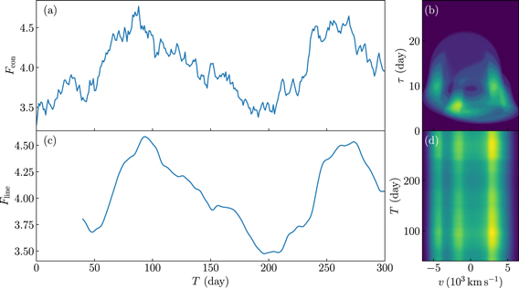
Figure 13. Simulated light curves of continuum and emission lines. Panel (a) is the continuum light curve generated by the damped random walk model. Panel (b) is the 2D TF of a typical CB-SMBH. Convolving the continuum light curve with the 2D TF, we obtain the 1D and 2D light curve of the emission line in panels (c) and (d), respectively.
Download figure:
Standard image High-resolution imageIn the simulations, the uncertainties of the continuum are fixed to 1%. We modify the emission-line profiles to evaluate the influence of two observational factors:
- The spectral resolution is dominated mainly by the line-spread function (instrumental broadening). To obtain observed profiles of different spectra resolutions, we convolve the simulated line profiles with a Gaussian broadening function B(λ):. The spectra are sampled with intervals equal to half of the FWHM of B(λ).
- At every data point Lℓ(v, t) of the line profile, a random number
is drawn from a Gaussian distribution with standard deviation σ = (S/N)−1. The observed noisy data point is then
.


We enhance the resolution from 1000 to 8000 (by factors of 2) and increase the S/N from 25 to 100 (by factors of 2) to generate different simulated RM data. The MEM-reconstructed 2D TFs from simulated RM data are shown in Figure 14. The implementation of MEM is briefly introduced in the Appendix. When the spectral resolution is ≥4000 and the S/N of the profile is ≥50, the superposition of the two bell shapes can be seen from the reconstructed 2D TF. There are three discrete bright parts in the 2D TF, corresponding to the edge of the bell-shaped TF: the left one is the blue side of the Keplerian disk of the primary BH; the middle one is the blue side of the secondary BLR; and the right one is the overlap of the red sides of the two BLRs. The overlap of the red side indicates that the phase angle is between 0° and 90°. Compared with the atlas in Figure 4, we can conclude that the inclination must be larger that 15°, unless all bright parts of the TF are mixed with each other. From the relative size and strength of the two bell shapes, we can also infer that the mass fraction of the primary BH must be smaller than 0.8.
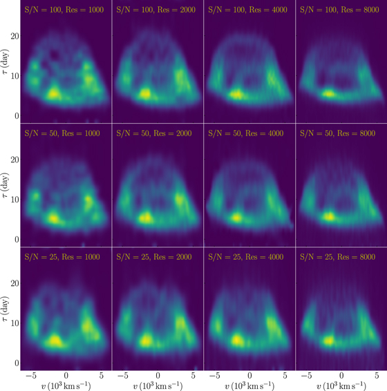
Figure 14. Reconstructed 2D TFs by MEM from simulated data with different S/N and spectral resolution. When the spectral resolution ≥4000 and S/N ≥ 50, typical features of the CB-SMBH will be present in the reconstructed 2D TF.
Download figure:
Standard image High-resolution imageClearly, given enough S/N and spectral resolution, it is possible to select CB-SMBH candidates by comparing reconstructed 2D TFs from RM data with our atlases. Furthermore, detailed comparison can also indicate the basic geometry and kinematics of the binary BLRs and give loose constraints on some model parameters.
6. Conclusions
We address the problem of whether reverberation mapping can be used to identify binary BLRs in CB-SMBHs. Given separated BLRs of binary BHs ionized by their own accretion disks, we demonstrate that the total TF is the linear superposition of the individual TFs of two BLRs, so long as the continuum light curves can be describe by a DRW, and the timescale of variation is much shorter than the time span of the light curve but longer than the cadence. When linear superposition holds, reverberation mapping of CB-SMBHs can be parameterized by a simple model in which the BLR is characterized by a Keplerian, inflowing, or outflowing disk. We provide atlases of 2D TFs for a wide range of geometries and kinematics. If the spectral resolution is larger than 4000 and the error is less than 2%, 2D TFs reconstructed from RM data using MEM can be compared with our atlases to select CB-SMBH candidates, constrain the geometry and kinematics of the BLRs, and, through detailed MCMC analysis, infer the probability distribution of model parameters.
We acknowledge the support by National Key R&D Program of China (grants 2016YFA0400701 and 2016YFA0400702), by NSFC through grants NSFC-11873048, -11833008, -11573026, -11473002, -11721303, -11773029, -11833008, -11690024, and by grant No. QYZDJ-SSW-SLH007 from the Key Research Program of Frontier Sciences, CAS, by the Strategic Priority Research Program of the Chinese Academy of Sciences grant No. XDB23010400.
Appendix: Maximum Entropy Method
MEM is proven to be effective in recovering the 2D TFs from the reverberation signal (e.g., Bentz et al. 2010; Grier et al. 2013; Xiao et al. 2018b; Mangham et al. 2019). We introduce a discrete linearized echo model ![${L}_{{\ell }}({v}_{i},{t}_{k})={\bar{L}}_{{\ell }}({v}_{i})\,+{\sum }_{j}{\rm{\Psi }}({v}_{i},{\tau }_{j})\left[{L}_{{\rm{c}}}({t}_{k}-{\tau }_{j})-{\bar{L}}_{{\rm{c}}}\right]{\rm{\Delta }}\tau $](https://content.cld.iop.org/journals/0067-0049/247/1/3/revision1/apjsab665aieqn65.gif) to fit the light curve of continuum and velocity-resolved emission lines, and to recover the 2D TF Ψ(vi, τj) simultaneously. Here
to fit the light curve of continuum and velocity-resolved emission lines, and to recover the 2D TF Ψ(vi, τj) simultaneously. Here  is the background spectrum to be fitted, and
  is the referenced continuum level that is fixed to the median of the continuum data. The MEM fitting is accomplished by varying the model parameters
  to minimize the quantity Q = χ2 − αS. Here,
 ![${\chi }^{2}={\sum }_{m}{\left[{D}_{m}-{{\mathscr{M}}}_{m}({\boldsymbol{p}})\right]}^{2}/{\sigma }_{m}^{2}$](https://content.cld.iop.org/journals/0067-0049/247/1/3/revision1/apjsab665aieqn69.gif) controls the differences between the data Dm and the model prediction
controls the differences between the data Dm and the model prediction  , entropy
 ![$S={\sum }_{n}\left[{p}_{n}-{q}_{n}-{p}_{n}\mathrm{ln}({p}_{n}/{q}_{n})\right]$](https://content.cld.iop.org/journals/0067-0049/247/1/3/revision1/apjsab665aieqn71.gif) is introduced in the MEM fitting to ensure the “smoothness” of the model parameters pn, and qn is designed as the “default value” of pn and set to weighted averages of “nearby” parameters. For example,
is introduced in the MEM fitting to ensure the “smoothness” of the model parameters pn, and qn is designed as the “default value” of pn and set to weighted averages of “nearby” parameters. For example,  for the one-dimensional (1D) models.
MEM has four user-controlled parameters:  and
and  , which control the trade-off between χ2 and S, the aspect ratio of Ψ(v, τ), and the “stiffness” of Ψ(v, τ) and Lc(t), respectively. Details of the parameter selections can be found in Xiao et al. (2018a). In our simulation, we fix the values of
  and
and  to 1 to guarantee the same level of features in Ψ(v, τ) and Lc(t), and vary the value of α to get similar χ2 in the fittings of data with different S/N and spectral resolution.
Footnotes
- 6