The Astrophysical Journal Supplement Series

The following article is Open access

An Overview of Solar Orbiter Observations of Interplanetary Shocks in Solar Cycle 25

Domenico Trotta, Andrew Dimmock, Heli Hietala, Xochitl Blanco-Cano, Timothy S. Horbury, Rami Vainio, Nina Dresing, Immanuel Christopher Jebaraj, Francisco Espinosa Lara, Raúl Gómez-Herrero

Published 2025 February 10 • © 2025. The Author(s). Published by the American Astronomical Society.
The Astrophysical Journal Supplement Series, Volume 277, Number 1Citation Domenico Trotta et al 2025 ApJS 277 2DOI 10.3847/1538-4365/ada4a7

PDF Opens in a new tab.

Article metrics

2559 Total downloads
0 Video abstract views

Dates

Received 2024 October 31
Revised 2024 December 15
Accepted 2024 December 30
Published 2025 February 10

Unified Astronomy Thesaurus concepts

Interplanetary shocks; Space plasmas; Solar activity; Interplanetary particle acceleration

Journal RSS

Create or edit your corridor alerts

What are corridors?

Abstract

Interplanetary (IP) shocks are fundamental constituents of the heliosphere, where they form as a result of solar activity. We use previously unavailable measurements of IP shocks in the inner heliosphere provided by Solar Orbiter, and present a survey of the first 100 shocks observed in situ at different heliocentric distances during the rising phase of solar cycle 25. The fundamental shock parameters (shock normals, shock normal angles, shock speeds, compression ratios, Mach numbers) have been estimated and studied as a function of heliocentric distance, revealing a rich scenario of configurations. Comparison with large surveys of shocks at 1 au shows that shocks in the quasi-parallel regime and with high speed are more commonly observed in the inner heliosphere. The wave environment of the shocks has also been addressed, with about 50% of the events exhibiting clear shock-induced upstream fluctuations. We characterize energetic particle responses to the passage of IP shocks at different energies, often revealing complex features arising from the interaction between IP shocks and preexisting fluctuations, including solar wind structures being processed upon shock crossing. Finally, we give details and guidance on the access use of the present survey, available on the EU-project “Solar Energetic Particle Analysis Platform for the Inner Heliosphere” website. The algorithm used to identify shocks in large data sets, now publicly available, is also described.

Export citation and abstractBibTeX RIS

Previous article in issue

Next article in issue

Original content from this work may be used under the terms of the Creative Commons Attribution 4.0 licence. Any further distribution of this work must maintain attribution to the author(s) and the title of the work, journal citation and DOI.

1. Introduction

Shocks are ubiquitously observed in astrophysical environments, where they are believed to play a crucial role in energy conversion and particle acceleration (e.g., A. M. Bykov et al. 2019). Despite decades of research, the mechanisms by which shocks mediate such processes of energy conversion and particle acceleration are still a matter of debate (M. A. Lee et al. 2012). In general, shocks are abrupt transitions between supersonic and subsonic flows, converting directed bulk flow energy (upstream) into heat and magnetic energy (downstream) (A. Marcowith et al. 2016). In the collisionless case, a fraction of the available energy can be channeled in the production of energetic particles (e.g., L. O. Drury 1983).

Heliospheric shocks are unique as accessible by direct spacecraft observations, and thus represent the missing link to astrophysical systems only observable remotely, like in the case of spectacular radiation emission due to shock-accelerated particles in supernova remnants (e.g., R. Giuffrida et al. 2022). Most of our knowledge is built around direct observations of the Earth's bow shock, resulting from the interaction between the supermagnetosonic solar wind and the Earth's magnetosphere, which represents an obstacle to its propagation (J. P. Eastwood et al. 2015). Since the early predictions and evidence due to the IMP8 mission (J. W. Dungey 1979) to the modern NASA Magnetospheric MultiScale mission (MMS; J. L. Burch et al. 2016) elucidating the details of how energy is partitioned across the shock transition (S. J. Schwartz et al. 2022), the Earth's bow shock has been an invaluable resource to understand shock behavior down to the smallest, kinetic scales. In the past decades, particles reflected by the Earth's bow shock and the fluctuation they induce in the upstream plasma (namely, particle and wave foreshocks) have been extensively documented using the large spacecraft fleet now orbiting Earth (see, for example, W. P. Wilkinson (2003) and A. Lalti et al. (2022a) for detailed investigations performed with ESA Cluster (C. P. Escoubet et al. 1997) and NASA MMS). Such observational efforts have often been combined with numerical efforts to advance our understanding of a variety of phenomena where shocks play a central role (e.g., Y. Y. Kartavykh et al. 2013; L. Turc et al. 2023).

Interplanetary (IP) shocks travel in the heliosphere driven by eruptive phenomena like coronal mass ejections (CMEs) and solar wind stream interaction regions (SIRs) (L. F. Burlaga 1971; I. G. Richardson 2018; D. F. Webb & T. A. Howard 2012). IP shocks are much less investigated than the Earth's bow shock due to several observational challenges, due to their higher speed with respect to the Earth's bow shock posing a stronger constraint on needed time resolution to resolve the shock transition, and due to the lower number of multispacecraft observations (I. J. Cohen et al. 2019). Therefore, IP shocks allow us to access a poorly explored regime of shock dynamics, including shock evolution from their origin at the Sun and into the IP medium (J. D. Richardson 2011). IP shocks are typically weaker and with larger radii of curvature compared to the Earth's bow shock (e.g., D. V. Reames 1999), and their waves and particle foreshocks are much less well characterized than their terrestrial counterparts, with several studies highlighting fundamental differences between them. For example, using the Solar Terrestrial Relations Observatory (STEREO) mission (M. L. Kaiser et al. 2008), P. Kajdič et al. (2012) have shown that upstream waves are somewhat irregular at IP shocks, and are sometimes observed without corresponding shock-reflected particle populations as would be expected. X. Blanco-Cano et al. (2016) surveyed IP shocks observed by STEREO from 2007 to 2010 and showed that significant suprathermal particle populations are more likely to be found at CME-driven shocks at 1 au with respect to SIR-driven ones due to different evolutionary features of such structures. Transient structures, routinely observed at the Earth's bow shock and known to play a fundamental role in energy conversion and particle acceleration (F. Plaschke et al. 2018), are very rarely observed at IP shocks, with little evidence of upstream shocklets (E. A. Lucek & A. Balogh 1997; L. B. Wilson et al. 2009; D. Trotta et al. 2023a) and downstream jets (H. Hietala et al. 2024).

Additionally, IP shocks provide insights into how the shock system evolves in time and through its spatial propagation, an aspect that cannot be investigated for the Earth's bow shock. From this point of view, multispacecraft observations leveraging different heliospheric vantage points are crucial to reconstruct fundamental properties of the shock system (N. Lugaz et al. 2024). Crucially, novel missions like NASA's Parker Solar Probe (PSP; N. J. Fox et al. 2016) and ESA's Solar Orbiter (D. Müller et al. 2020) are probing the inner heliosphere with state-of-the-art instrumentation, thereby yielding previously unavailable data sets and therefore provide an unprecedented opportunity for discovery in IP shocks. The importance of such inner heliospheric observers has been highlighted by several recent works exploiting useful lineups among them and the existing near-Earth spacecraft fleet (e.g., D. Trotta et al. 2024a, 2024b; E. E. Davies et al. 2024). Furthermore, the exploitation of this tantalizing observational window is particularly timely given the peak of activity of solar cycle 25, modulating IP shock occurrence (S. Y. Oh et al. 2007) and motivating shock surveying efforts providing opportunities to study the most interesting events of the solar cycle as well as stimulating discussion around the general trends and occurrence of shocks through different phases of solar activity. (see, for example, D. M. Oliveira 2023).

In this work, we present an extensive survey of IP shocks observed at different heliocentric distances using Solar Orbiter. The shock survey has been carried out within the framework of the European Project Solar Energetic Particle Analysis Platform for the Inner Heliosphere (SERPENTINE¹⁴ ), and is publicly available through the project data center.¹⁵ The version discussed here is citable through Zenodo (D. Trotta et al. 2024c). In Section 2, we present the data sets used. Section 3 describes the methods of shock identification and characterization used throughout the survey, discussing the key parameters computed for each event and summarizing the information provided for each observed IP shock. In Section 4, we describe the first results of this statistical effort, showing the general trends of shock parameters with heliocentric distance and in relation to previous observations at 1 au (Section 4.1). We also discuss the general properties of wave foreshocks and the energetic particle response to the passage of IP shocks as observed by the novel Solar Orbiter payload (Sections 4.2 and 4.3, respectively). In Section 5, we present the conclusions. Finally, in Appendices A and B we give details about shock search software developed and used here and about how to use this catalog and its future implementation through the SERPENTINE data center.

2. Data

We exploit the full in situ suite on board the Solar Orbiter mission (D. Müller et al. 2020). To measure the magnetic field, we use the flux-gate magnetometer (MAG; T. S. Horbury et al. 2020), yielding magnetic field measurements at up to 64 vectors s⁻¹. Low-energy ion energy flux has been measured with the Proton Alpha Sensor (PAS) of the Solar Wind Analyser suite (SWA; C. J. Owen et al. 2020), yielding measurements at 4 s resolution in the 200 eV–20 keV range. For ion bulk flow speed, density, and temperature, we used the PAS ground moments at 4 s resolution. In some cases, density estimates from the Radio and Plasma Waves instrument (M. Maksimovic et al. 2020) are also used. Several sensors of the Energetic Particle Detector suite (EPD; J. Rodrìguez-Pacheco et al. 2020) have been used: the SupraThermal Electrons and Protons (STEP) sensor, Electron Proton Telescope (EPT) and High Energy Telescope (HET), continuously measuring energetic electrons and protons from the suprathermal regime (2 keV for electrons) to low-energy galactic cosmic-ray energies of 100 MeV/n at high time resolutions, up to 1 s. EPT and HET comprise four telescopes with different look directions, sunward, anti-sunward, north, and south, respectively. The STEP detector, instead, comprises 15 pixels and its look direction overlaps with the EPT–HET Sun viewing direction.

3. The Solar Orbiter Shock List

In this section, we describe the process of shock identification and characterization performed to compile the Solar Orbiter shock list. Our search starts shortly after the mission launch in spring of 2020 and is now up to date until 2023 December 31, containing 100 events at heliocentric distances between 0.3 and 1 au. Figure 1 shows an overview of the Solar Orbiter trajectory from 2020 April to 2024 January, in a frame of reference where Earth and the Sun are fixed (blue and yellow circles, respectively). The red dots represent the events identified, elucidating how small heliocentric distances are covered, an important complement to knowledge built on events at 1 au.

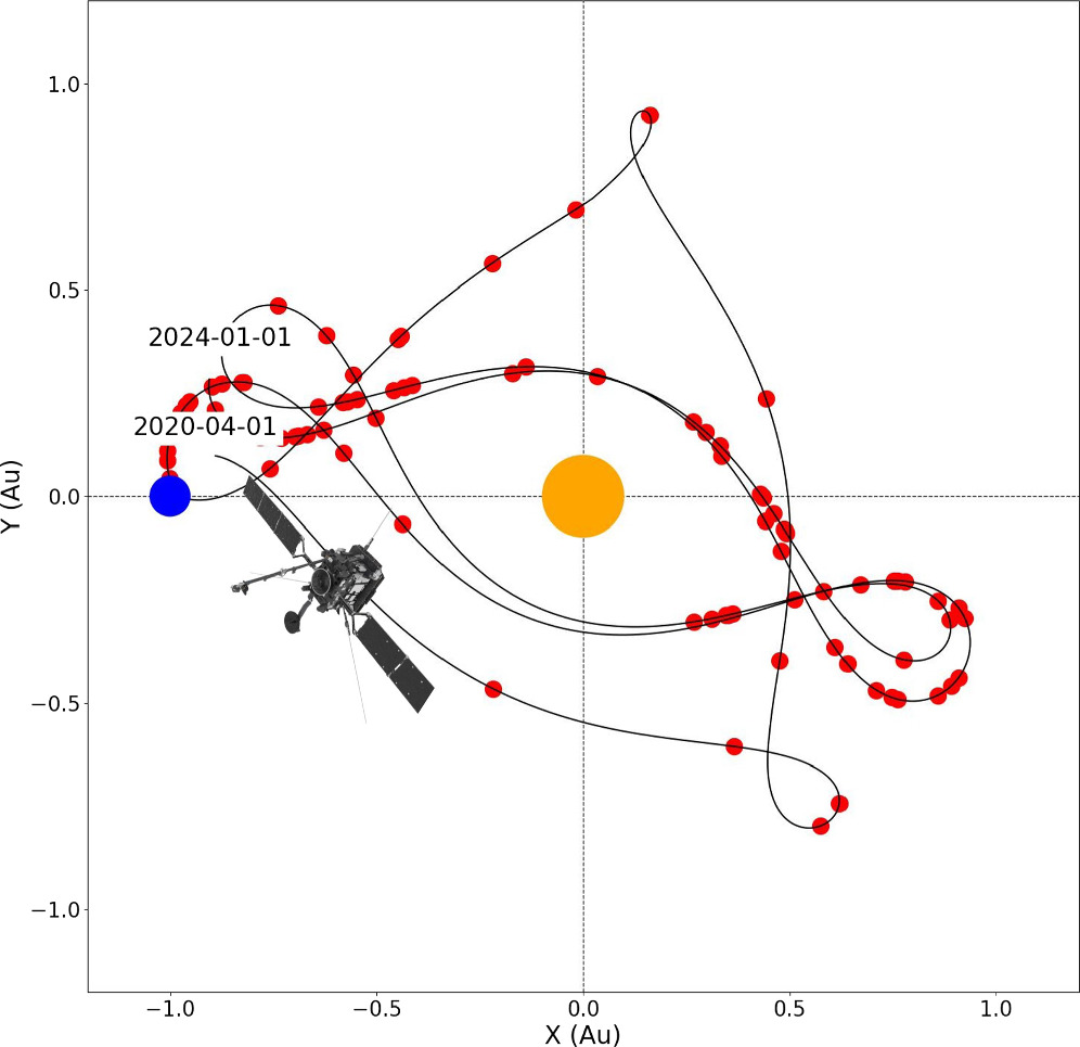
Figure 1. Refer to the following caption and surrounding text. — **Figure 1.** Solar Orbiter trajectory (black line) throughout our statistical campaign in a fixed Earth–Sun frame. The red dots represent IP shock crossings, and the blue and yellow dots represent the Earth and the Sun, respectively. (Solar Orbiter model: https://www.esa.int/).
Download figure:
Standard image High-resolution image

3.1. Shock Identification

Shocks can be viewed as discontinuities and, therefore, sudden changes in the plasma conditions. In this picture, identifying shocks and characterizing their statistical properties in the large data sets provided by modern spacecraft missions becomes a nontrivial task because the sudden changes in the plasma properties mentioned above occur on extremely short (approximately seconds) timescales.

Motivated by this fascinating “big data problem” of finding small-scale (approximately seconds) structures in long time series (approximately years), and in the spirit of the SERPENTINE project representing a platform for the community to study energetic particles and their origins, we decided to develop software to identify such shock transitions in spacecraft data. This software package, Tracking and Recognition of Universally Formed Large-scale Shocks (TRUFLS), is publicly available on GitHub¹⁶ and described in detail in Appendix A. The majority of Solar Orbiter shocks in this work were identified with TRUFLS, which is designed to work as well with other missions yielding in situ magnetic field and plasma data. Once candidates are identified and confirmed visually, a full characterization of the event is performed, as discussed in Section 3.2. Waves and energetic particles are also thoroughly characterized, as reported in Sections 4.2 and 4.3, respectively.

Other means of identification are used to ensure the list is complete and up to date. To this end, magnetic field-only candidates, particularly in the early stages after the launch of Solar Orbiter, when SWA suffered frequent interruptions in its operations, we often spotted by visual inspection and flagged in the list as “magnetic field only.” Furthermore, we regularly cross-checked our shock list with the ICME catalog “ICMECAT” built within the HELIO4CAST project (C. Mstl et al. 2017), accessible at the HELIO4CAST web page. ¹⁷

3.2. Shock Parameter Estimation Techniques

The structure and behavior of collisionless shocks are regulated by several parameters, one of the most important being the angle between the normal of the shock surface and the upstream magnetic field θ_Bn (e.g., D. Burgess & M. Scholer 2015). For θ_Bn values close to 90°, i.e., when the upstream magnetic field is almost tangential to the shock surface, the shock is quasi-perpendicular. On the other hand, for θ_Bn values close to 0° (corresponding to an upstream magnetic field almost normal to the shock surface), the shock is quasi-parallel. Particle reflection and propagation far upstream is favored at quasi-parallel shocks (C. F. Kennel et al. 1985), introducing the possibility for reflected particles to interact with the upstream plasma over long distances, creating unstable distributions and a collection of disturbances in the plasma properties, giving rise to the so-called particle and wave foreshocks (e.g., J. P. Eastwood et al. 2005).

Other important parameters that dictate the behavior of collisionless shocks are the (Alfvénic and fast magnetosonic) Mach number, i.e., the ratio between the shock speed in the upstream flow frame (v_sh) and the upstream Alfvén (v_A) and fast magnetosonic (v_fms) speeds, respectively (M_A ≡ v_sh/v_A and M_fms ≡ v_sh/v_fms). The upstream plasma beta, i.e., the ratio between the plasma and magnetic field pressure, often expressed as a ratio of squared thermal and Alfvén speeds $\beta \equiv {{v}}_{{\rm{th}}}^{2}/{{v}}_{{\rm{A}}}^{2}$ , and the gas and magnetic compression ratios (r_Gas ≡ n_d/n_u and r_B ≡ B_d/B_u, respectively, where the d and u subscripts indicate the downstream and upstream states) are also relevant for shock dynamics.

Shock parameter estimation using single spacecraft crossings is often a challenging task due to the intrinsic three-dimensional nature of the system and the fluctuations typically involved in the transitions (e.g., A. Koval & A. Szabo 2008). Throughout this work, we used different methods to determine shock parameters. The shock normal (and therefore the θ_Bn) estimation is done using the mixed-mode 3 method, consistent with previous catalogs (E. K. Kilpua et al. 2015). When plasma data is not available, the magnetic coplanarity method is used to determine the shock normal vector. The shock speed along its normal is computed using the mass flux conservation, and it is given in the spacecraft frame of reference. A comprehensive summary of the above techniques can be found in G. Paschmann & S. J. Schwartz (2000). From these estimations, further shock parameters are determined (e.g., Mach numbers, compression ratios), as summarized in Table 1.

Table 1. Summary of the Shock Properties and Parameters Provided in the Solar Orbiter Shock List

Parameter	Content	Units
Shock ID	Shock unique identifier	⋯
Shock date	Date of shock observation	UT
Shock time	Time of the shock crossing	UT
Heliocentric distance	Distance from the Sun	au
Solar-MACH configuration	Link to orbit configuration plot	⋯
Associated SEP event	ID of associated SEP event	⋯
Mean upstream δB/B₀	δB/B₀ (lag: 1 minute)	⋯
Upstream density	Mean upstream ion density	cm⁻³
Upstream β	Mean upstream plasma beta	⋯
Upstream B	Mean upstream B vector	nT
${\hat{{n}}}_{\mathrm{shock}}$	Mean shock normal vector	⋯
θ_Bn	Mean shock normal angle	degrees
V_shock	Mean shock speed	km s⁻¹
M_A	Alfvénic Mach number	⋯
M_fms	Fast magnetosonic Mach number	⋯
r_B	Mean magnetic compression ratio	⋯
r_gas	Mean gas compression ratio	⋯
Structures—2 hr	Structuring across shock	⋯
Structures—8 minutes	Structuring across shock	⋯
Notes	E.g., data availability	⋯
Identified with	E.g., TRUFLS, visual inspection	⋯
Possibility of multispacecraft observation	Other spacecraft within 0.2 au	⋯
Wave foreshock	Present/absent	⋯
Foreshock extent	Duration of wave foreshock	minutes
Frequency range	Frequencies of enhanced wave activity	Hz
Low-energy particle reflection	Present/Absent	⋯
Proton response at selected energies	No response/spike/plateau/irregular	⋯
Proton peak delay t_peak − t_shock	For selected energies	minutes
Electron response at selected energies	⋯	⋯
Notes on particle response	⋯	⋯

Note. An interactive and downloadable list can be found on the SERPENTINE data center (see Appendix B).

Download table as: ASCII Typeset image

Crucially, single spacecraft shock parameter estimations involve an operation of averaging upstream/downstream of the shock crossing, making the results particularly sensitive to the choice of averaging windows. Furthermore, the shock normal determination is particularly sensitive to the choice of averaging, introducing an uncertainty that propagates to shock speed and Mach number estimations carried out in the shock normal frame (G. Paschmann & S. J. Schwartz 2000). Building on the idea first proposed in A. Balogh et al. (1995), we developed a technique involving a systematic variation of upstream/downstream averaging windows and yielding distributions of shock parameters that can be used to determine uncertainties (see D. Trotta et al. 2022a, for details). Shock parameters in this catalog have been computed with such a technique, implemented within the SERPENTINE project in the publicly available SerPyShock code.¹⁸ The length of the averaging windows was systematically varied from 30 s to 8 minutes both upstream and downstream, compatible with fixed windows previously used in other catalogs (E. K. Kilpua et al. 2015).

The Solar Orbiter shock list is publicly available on the SERPENTINE data center, where interactive access and a series of quick-look plots are also included. These are detailed in Appendix B. In Table 1, we summarized the quantities reported in the list and used in the present work. It may be noted that the structure of the list can be divided into three parts: identification and context, shock parameters, and wave and energetic particle response (top to bottom in Table 1).

The link to the Solar-MACH configuration plot (entry 5 in Table 1, available in the online version of the catalog) uses the Solar Magnetic Connection HAUS tool (J. Gieseler et al. 2023), yielding the orbital configuration for the event. Additionally, we provide information regarding the association with solar energetic particle (SEP) events referring to the solar cycle 25 multispacecraft SEP event catalog of the SERPENTINE project (N. Dresing et al. 2024a), also available through the SERPENTINE data center.¹⁹ The mean upstream δB/B₀, density, plasma β, and magnetic fields are evaluated in the 8 minutes before the shock. This choice is fixed for all events, to ensure reproducibility and the possibility to seamlessly integrate new events in the future. A case-by-case procedure, based on the visual inspection of each event, is also reported in Appendix C.

4. Results

In this section, we show the outcomes of the identification and characterization described in Section 3 for the first 100 Solar Orbiter shocks detected from 2020 to 2023 at heliospheric distances spanning 0.3–1 au.

4.1. Overview

Figure 2 shows an overview of shock parameters for all the 100 events in the list. Typical features of IP shocks are recovered here, as described below. Alfvénic and fast magnetosonic Mach numbers are mostly moderate (≤3), confirming that IP shocks tend to be weaker than the Earth's bow shock (e.g., A. Lalti et al. 2022a). Both gas and magnetic field compression ratios are systematically lower than 4 (e.g., E. J. Smith 1985; D. Lario et al. 2005; E. K. Kilpua et al. 2015; C. A. Pérez-Alanis et al. 2023). This is consistent with the limit imposed by the MHD theory, where the shock compression ratio is limited to 4 (e.g., M. Kivelson & C. Russell 1995). However, it can be seen that in some observations, a gas compression ratio larger than 4 is observed, an effect that may be due to the one-dimensional nature of the observations sampling regions connected differently to the shock (e.g., G. Paschmann & S. J. Schwartz 2000), as well as to kinetic effects beyond the MHD limiting value of 4 (D. Burgess & M. Scholer 2015). The distribution of shock normal angles θ_Bn (Figure 2(c)) shows that the quasi-perpendicular geometry (θ_Bn≥ 45°) is favored for IP shocks. This effect is probably due to two factors, namely the global configuration of the magnetic field the shocks propagate through (J. K. Chao & Y. H. Chen 1985; D. V. Reames 1999; M. Janvier et al. 2014), and a selection bias because quasi-parallel shocks are more challenging to identify due to the fact that magnetic compression goes to zero for θ_Bn approaching zero, and the quasi-parallel shock environment is much more disturbed than the perpendicular one (O. Kruparova et al. 2013; D. M. Oliveira 2023). However, the high-resolution magnetic field measurements yielded by the MAG instrument (T. S. Horbury et al. 2020) mitigate this problem and, when identified, yield invaluable information about the behavior of such shock transitions (see, for example, A. Dimmock et al. 2023; D. Trotta et al. 2023a). In Figure 2(f), we show the distribution of shock speeds. In this plot, shocks with negative speed are fast reverse (FR) shocks, which rarely occur in the inner heliosphere with respect to 1 au and beyond (R. Schwenn 1996; L. Jian et al. 2006). However, given the high level of solar activity, some reverse shocks may be observed, for example, due to CME–CME interactions, as recently shown in D. Trotta et al. (2024b). Finally, in Figures 2(g)–(i), we show the orientations of the local shock normals, in the RTN frame of reference, for all the events. It may be noted that the local shock normal vectors exhibit a strong variability, indicating that strong departures from the radial directions are routinely observed locally, thus highlighting the variability of the shock system.

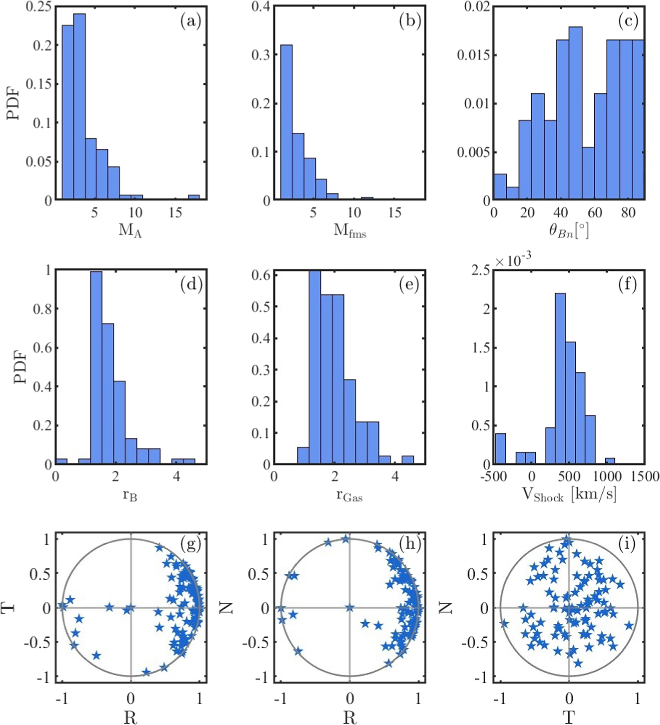
Figure 2. Refer to the following caption and surrounding text. — **Figure 2.** Overview of shock parameters for all the shocks identified. The panels show PDFs of Alfvénic and fast magnetosonic Mach numbers M_A, M_fms, shock normal angle θ_Bn, magnetic and gas compression ratios r_B, r_gas, and shock speed V_shock (a)–(g), respectively). Panels (g)–(i) show scatters of shock normal vectors in the RTN frame.
Download figure:
Standard image High-resolution image

In Figure 3, we further exploit the Solar Orbiter capabilities in probing the inner heliosphere, showing the shock parameters for all the events as a function of heliocentric distance. Heliocentric distances where Solar Orbiter spent a limited time, and therefore identified only a few shocks, are highlighted by the orange-shaded panels. As shown in Figure 3, no strong trends can be identified for shock parameters at different heliocentric distances, except for θ_Bn going toward more perpendicular geometries with increasing heliocentric distance, as described above. There is, however, a small indication that the three shocks identified near perihelion (0.3 au) may be relatively strong, an effect that could be related to faster CMEs driving such shocks in the inner heliosphere (e.g., L. A. Balmaceda et al. 2020, and references therein). These results indicate that the local shock behavior is poorly influenced by the shock age and/or different global heliospheric configurations, with important implications for energetic particle production in the heliosphere.

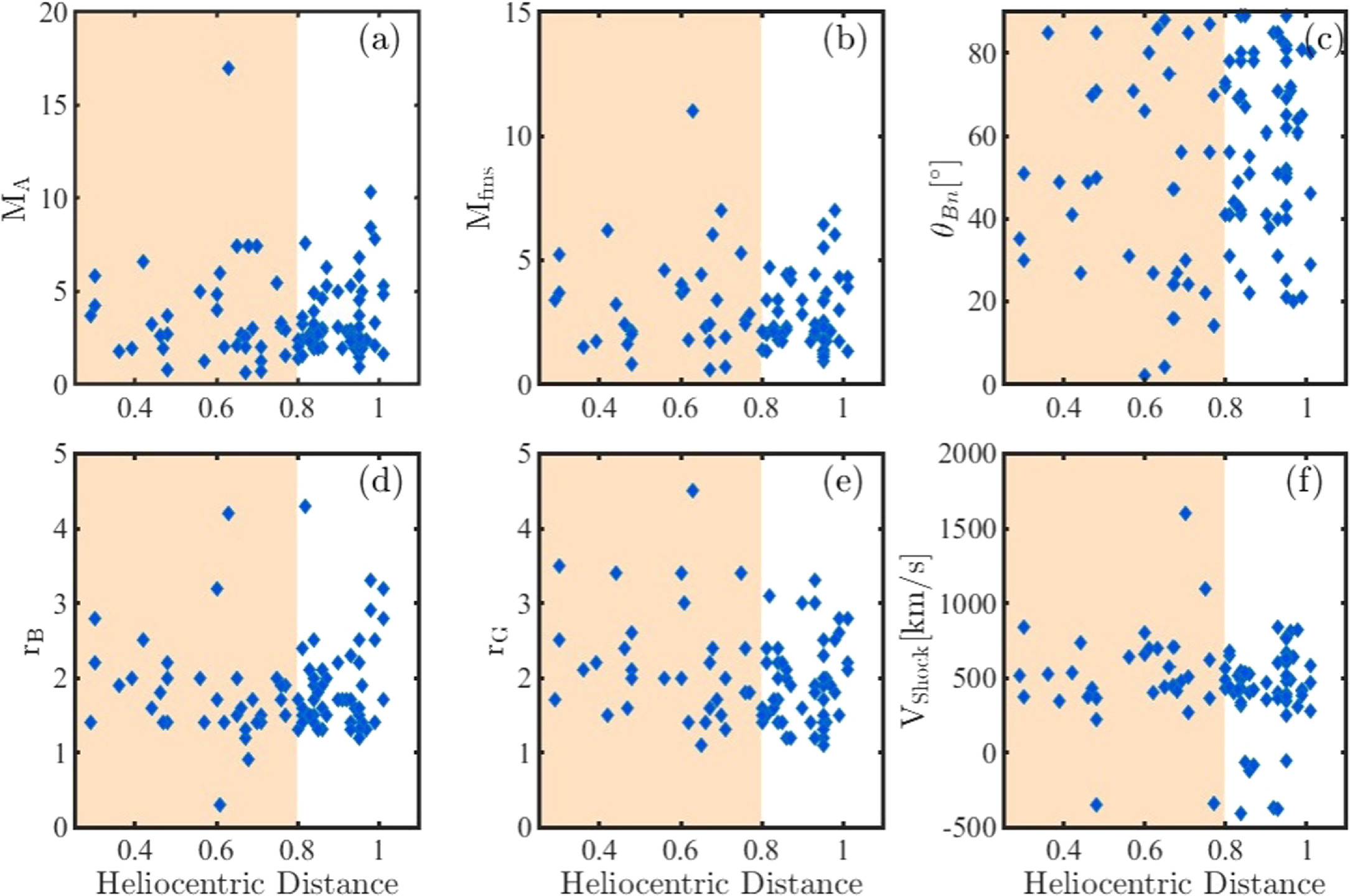
Figure 3. Refer to the following caption and surrounding text. — **Figure 3.** Shock parameters as a function of heliocentric distances in astronomical units. The parameters shown in panels (a)–(f) follow from the same panels in Figure 2. The orange-shaded panels highlight poorly investigated heliocentric distances.
Download figure:
Standard image High-resolution image

To take the characterization of inner heliospheric shocks further, we filtered the sample based on heliocentric distance and isolated 30 fast forward (FF) shocks below 0.8 au and compared them with 586 FF shocks observed with STEREO-A and Wind between 1995 and 2009, a very large sample reported in E. K. Kilpua et al. (2015). Results for selected shock parameters are shown in Figure 4. It can be seen that there are no significant deviations from the overall behavior at 1 au, apart from a slight trend in θ_Bn (Figure 4(a)), in which more parallel configurations are favored at low heliocentric distances. Such a trend in θ_Bn is explained by the large-scale orientation of the IP magnetic field at low heliocentric distances (J. K. Chao & Y. H. Chen 1985). Indeed, the Parker spiral is radial near the Sun (E. N. Parker 1958), explaining why the quasi-parallel configuration for IP shocks is easier to achieve. With the same argument, Voyager observations of IP shocks in the outer heliosphere show that the quasi-perpendicular geometry is greatly favored beyond 1 au (L. F. Burlaga 1994). Further, there is an indication of slightly higher shock speeds and fast magnetosonic Mach numbers in the inner heliosphere. This is possibly due to the fact that shock drivers are faster at short heliocentric distances, due to the drag effect causing CMEs to decelerate as they propagate in the heliosphere (e.g., C. Möstl et al. 2015). Effects beyond simple drag (e.g., C. Kay et al. 2022), as well as large-scale variabilities associated with the CME propagation (e.g., E. Provornikova et al. 2024) introduce additional complexities. However, we note that the observed trends are compatible with what was previously found on IP shock with the Helios mission (P. M. Volkmer & F. M. Neubauer 1985; H. R. Lai et al. 2012; R. Hajra et al. 2023). A more detailed investigation of radial trends with modern observatories will be the object of further work, including input from other important statistical studies using other inner heliospheric missions, such as Parker Solar Probe (N. J. Fox et al. 2016) and BepiColombo (J. Benkhoff et al. 2021), allowing in particular larger statistics of shocks closest to the Sun (∼0.5 au).

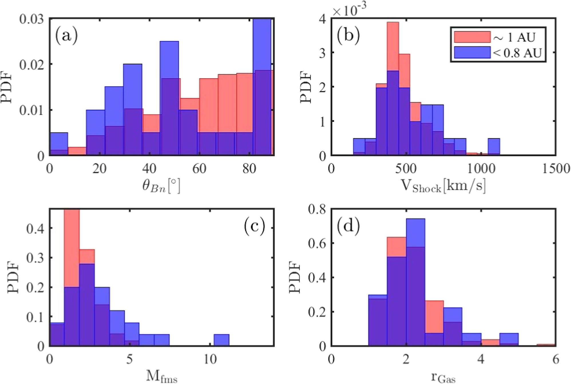
Figure 4. Refer to the following caption and surrounding text. — **Figure 4.** Comparison of shock parameters as observed by Solar Orbiter for 30 shocks at heliocentric distances smaller than 0.8 au (blue histograms) and 586 shocks observed from 1995 to 2009 at 1 au by E. K. Kilpua et al. (2015).
Download figure:
Standard image High-resolution image

4.2. Wave Environment

In this section, we briefly report on the wave environment observed at Solar Orbiter shocks. A detailed characterization of magnetic field fluctuations in correspondence to IP shock crossings has been performed for all the events in the Solar Orbiter shock list. The first quantity computed is the value of δB/B₀ close to the shock, computed as δB/B₀ ≡ ∣B(t + τ)− B(t)∣/∣B(t)∣, where the lag τ of 1 minute has been chosen (relevant to resonant scattering of protons with energies of around 100 keV) and then averaged for 8 minutes upstream. Furthermore, for each event, we study wavelet spectrograms of magnetic field intensity B and trace spectrograms of the magnetic field components. From the latter, the duration of the foreshock is estimated by visual inspection of intensity enhancement in correspondence with the crossing, specifying the range of wavelengths where such enhanced fluctuations are observed (see Table 1). Finally, to gain insights into the polarization of the observed waves, the reduced magnetic helicity, normalized by the power in magnetic field fluctuations ${\sigma }_{m}(k)\equiv {{kH}}_{m}^{(r)}(k)/{E}_{B}(k)$ (where k is the wavenumber, ${H}_{m}^{(r)}(k)$ is the reduced magnetic helicity (W. H. Matthaeus et al. 1982) and E_B(k) is the magnetic power spectral density) is also studied (T. A. Bowen et al. 2020; L. D. Woodham et al. 2021). Wave foreshocks result from the interaction of shock-reflected particles and the upstream plasma, where unstable distributions give rise to magnetic fluctuations extending far into the shock upstream, crucial for particle acceleration (e.g., D. Burgess & M. Scholer 2015). Another type of upstream wave, known as precursors, is often observed but generated by different shock physics. These waves are commonly observed between around 0.5 and 10 Hz, primarily classified as whistler waves, a branch of the fast magnetosonic wave. Whistler waves are also reported in the hundreds of Hz range but are not considered in these statistics. However, evidence of them has been observed in a few Solar Orbiter IP shocks (not shown).

Whistler waves can also be affected by Doppler shift (A. P. Dimmock et al. 2013), resulting in some variability in their frequency in the spacecraft frame. Whistler waves are a vital mechanism that aids the balancing of the nonlinear steepening of the ramp, predominantly observed around quasi-perpendicular shocks, and may be crucial for the first steps of electron acceleration (M. A. Riquelme & A. Spitkovsky 2011). There are still many open questions about their generation and role in energy conversion at the shock front. Since we do not identify the wave mode here, we will refer to these waves as low-frequency precursors. Many different publications have examined these precursors using various techniques and instruments, confirming they are both a critical component of the shock magnetic structure and intrinsically connected to particle dynamics across the shock. As expected, most analyses have benefited from decades of multispacecraft observations collected at the terrestrial bow shock (D. H. Fairfield 1974; A. P. Dimmock et al. 2013; A. Lalti et al. 2022b), leading to many noteworthy results that have significantly advanced our understanding of the role such waves play in collisionless shock dynamics. There have also been investigations of low-frequency precursors at different planets such as Venus (A. P. Dimmock et al. 2022), Mars (D. A. Brain et al. 2002), Saturn (A. H. Sulaiman et al. 2017), and Mercury (D. H. Fairfield & K. W. Behannon 1976). Moreover, they are also repeatedly observed in the solar wind close to IP shocks (L. B. Wilson et al. 2009), which is the focus of this paper. Our goal is to determine how many shocks in the Solar Orbiter database contain low-frequency precursors. To decide if low-frequency precursors are present, we inspect the wavelet power and ellipticity to check for enhancements and circular polarization in the relevant frequency range. The shocks for which no MAG burst or SWA-PAS data was available were excluded, resulting in 72 shocks to calculate this statistic. Based on the criteria above, visual assessment determines if a low-frequency precursor train is present.

Finally, we investigate, by visual inspection, the presence of preexisting structures such as flux ropes and discontinuities. Such structures, often neglected in theoretical modeling of particle acceleration, are emerging as a fundamental ingredient for particle acceleration (F. Guo et al. 2021). Indeed, the interaction of such preexisting structures with shocks may lead to enhanced energetic particle production, ranging from enhanced scattering upstream to downstream trapping (J. Giacalone et al. 2021; D. Trotta et al. 2020; E. Kilpua et al. 2023). In the catalog, the presence of such structures is reported for intervals in the 8 minutes and 2 hr around the shock (see Table 1).

Wave foreshocks have been identified in the frequency range between 0.01 and 1 Hz for 46% of the shocks. The duration of foreshocks has been found to vary from a few minutes to about one hour, depending on the preexisting structuring of the medium the shock propagates through. Indeed, long wave foreshocks have been found in cases where the shock propagates in plasma exhibiting low levels of preexisting magnetic fluctuations. One example is the long wave foreshock observed within CME material and documented in D. Trotta et al. (2024b). Extended wave foreshocks in such “quiet” environments are compatible with observations of long-lasting field-aligned beams of energetic particles, where scattering is inhibited under similar local plasma conditions (D. Lario et al. 2022). Similarly, we estimate that wave precursors are present in approximately 62% of shocks in this database, with the intriguing property of showing wave trains with significant changes in their duration. Solar Orbiter observations confirm that IP foreshocks tend to occur for low θ_Bn and high Mach numbers, a topic that will be expanded in further studies.

Figure 5 shows three examples of shocks with different wave environments. From top to bottom, we show the magnetic field vector components in spacecraft-centered RTN coordinates and magnitude, ion bulk flow speed and density, the trace wavelet power spectral density (PSD) spectrum of the magnetic field, the reduced magnetic helicity and the one-dimensional energy flux measured by PAS in a range of timescales ranging from a few minutes to about 3 hr. The case on the left column shows a shock with visible precursors, as shown in panels (e1) and (f1), where enhanced wavelet power and elliptical polarization are evident in the ∼2 minute interval preceding the shock crossing. In panel (f1), a red cluster indicates the circularly right-handed polarization. Their frequency in the spacecraft frame is around 3 Hz, and they are visible for up to 90 s upstream. This shock has θ_Bn = 67°, M_A = 2.8, and was observed at 0.8 au. In contrast, the shock in the middle column of Figures 5(a2)–(g2) has no clear indications of upstream precursors and any other wave activity upstream. This shock was observed around 0.8 au and had M_A = 2.4, similar to the first shock. However, this shock was almost perpendicular to θ_Bn = 86°. Another difference is that the second shock appears to have additional fluctuations downstream of the shock front compared to the first. Finally, the right side column of Figure 5 shows an IP shock with a wave foreshock lasting about 10 minutes observed at 0.44 au. This shock is quasi-parallel (θ_Bn ∼ 27°) and characterized by higher Mach numbers (M_A ∼ M_fms ∼ 3.2). The fluctuation enhancement is well visible in the wavelet spectrogram at frequencies between 0.01 and 1 Hz.

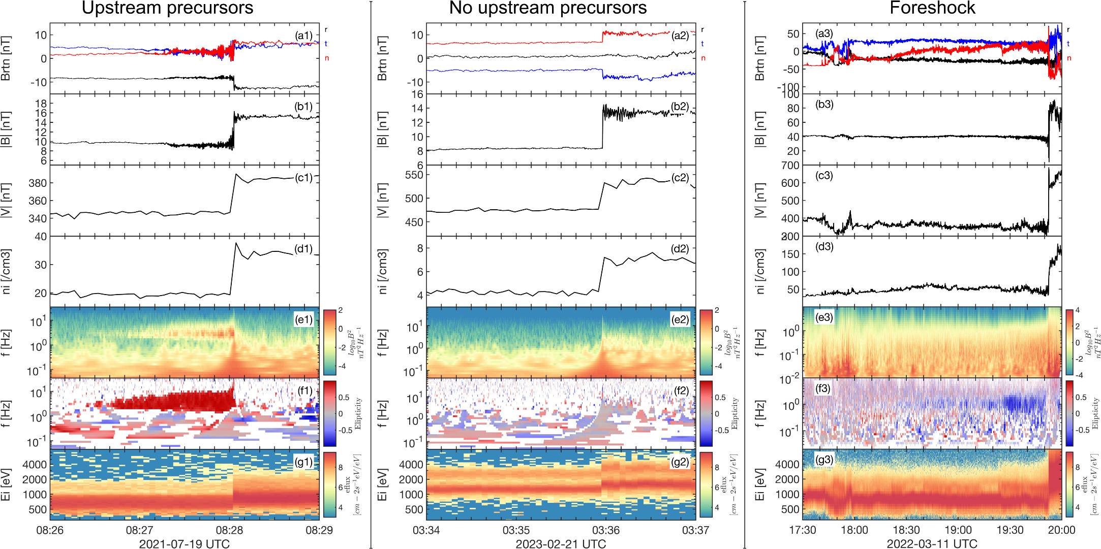
Figure 5. Refer to the following caption and surrounding text. — **Figure 5.** Examples of three IP shocks observed by Solar Orbiter exhibiting different wave environments. Panels (a)–(g) show B, ∣B∣, V, n_i, wavelet spectra, magnetic field ellipticity, and omnidirectional energy flux. The first case shows a clear upstream precursor (a1)–(g1), the middle one (a2)–(g2) shows no wave activity, and finally, the case on the right has an extended wave foreshock (a3)–(g3).
Download figure:
Standard image High-resolution image

Figure 5 shows how the variety in this database will help advance our understanding of low-frequency precursors’ appearance and their role in IP shocks. It will also allow IP shocks to be easily compared to databases collected in various other plasma environments (e.g., A. Lalti et al. 2022a; C. A. Pérez-Alanis et al. 2023).

One example of interesting comparison across different environments is the association of wave foreshocks with shock-reflected particles that can lead to unstable upstream distributions, as routinely observed at Earth's bow shock (H. Kucharek et al. 2004; M. Archer et al. 2005). Such association is often less clear for IP shocks. In Figure 6, we show two examples of wave and particle response to the passage of IP shocks. In the Figure, from top to bottom, we show the EPT-Sun, STEP, and PAS energy flux spectrograms (a)–(c), the trace magnetic field wavelet spectrogram (d), magnetic field magnitude and its RTN components (e), the magnetic field power spectral density collected in a 30 minute window immediately upstream of the shock and 2 hr before the shock arrival (green and orange lines, (f) panels), and one-dimensional ions energy fluxes collected for 4 and 30 minutes before the shock (green and orange points, (g) panels). On the left side of the figure, we show an oblique (θ_Bn ∼ 59°) shock with a low Mach number preceded by an extended (∼30 minutes) wave foreshock and an enhancement of suprathermal particles upstream. This event happens in an environment with a low level of magnetic fluctuations typical of CME material, and despite the low Mach number of the shock, provides an exceptional opportunity to study the interplay between upstream waves and shock-reflected particles (as reported in D. Trotta et al. (2024b) and X. Blanco-Cano et al. 2025, in preparation). In this case, despite the low Mach number of the shock, we find both an unusually long (∼30 minutes) wave foreshock and a population of shock-reflected particles upstream (Figures 6 (f1), (g1)). On the right side of the figure, we show a different case of a θ_Bn ∼ 41° shock, showing enhanced wave activity close (∼2 minutes) to the shock and up to 1 Hz (see Figure 6(d2)) but no suprathermal particle counterpart (Figure 6(g2)). Such a suprathermal counterpart was found instead in other cases with similar shock parameters case described in A. Dimmock et al. (2023). Figure 6 shows the emerging complexity of IP shocks, where many effects, ranging from time evolution to spatial irregularities and subsequent spacecraft connectivity to the shock surface (e.g., P. Kajdič et al. 2012) led to unexpected observations based on knowledge built on Earth's bow shock.

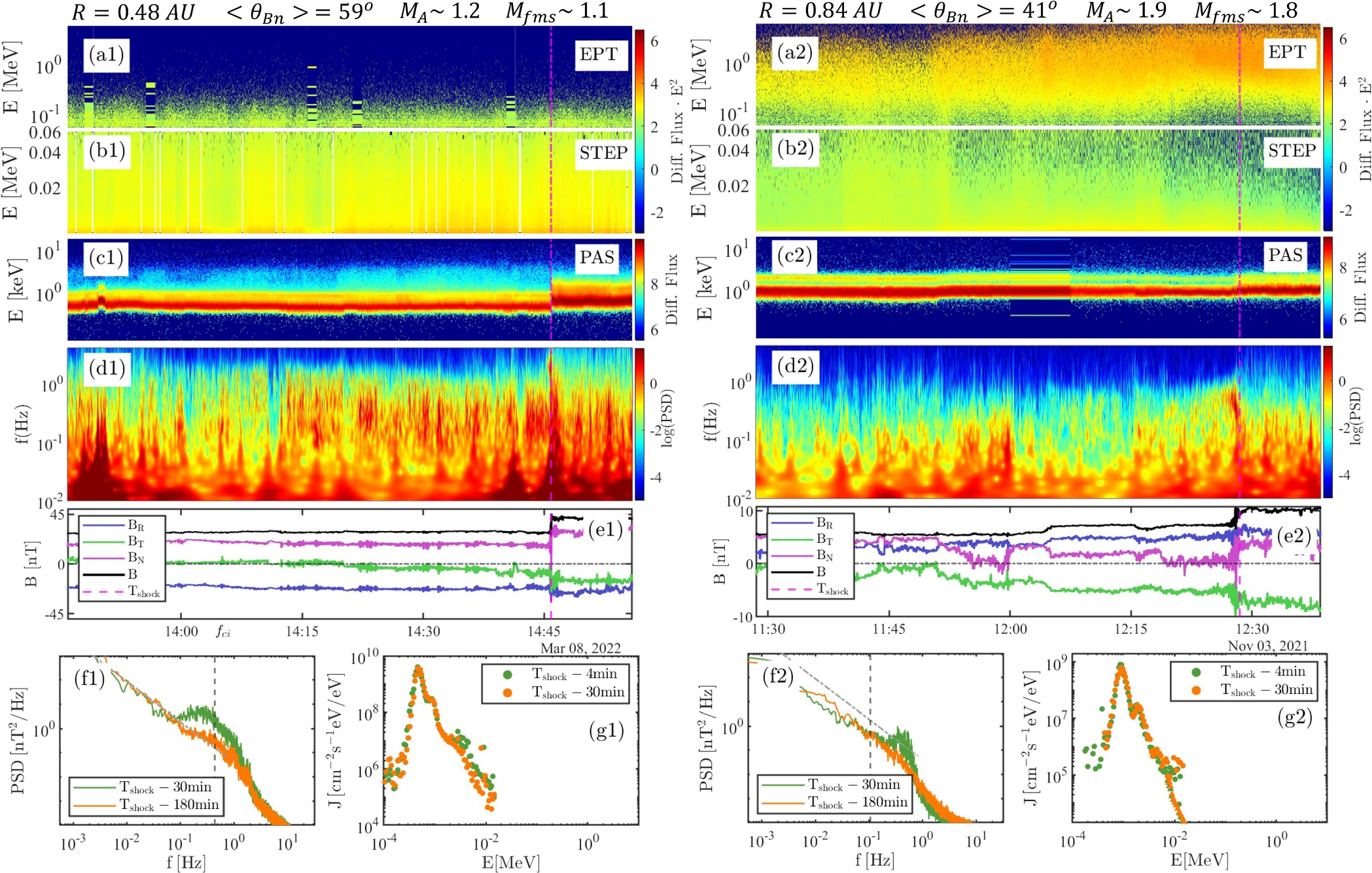
Figure 6. Refer to the following caption and surrounding text. — **Figure 6.** Wave and particle foreshocks for two different events. (a), (b) Energetic differential fluxes (in E² · cm⁻²s⁻¹sr⁻¹ MeV) as measured by EPD's Sun-directed EPT sensor (a) and STEP sensor (b). (c) Energy flux (in cm⁻²s⁻¹eV) measured by SWA-PAS. (d), (e) Magnetic field trace wavelet spectrogram (d) and magnetic field magnitude and components (e) measured by MAG. (f) Magnetic field PSD collected far (orange) and close (green) upstream of the shock. (g) PAS-EPD ion energy spectra were collected far (orange) and close (green) upstream of the shock. Example 1 shows both a wave and particle foreshock, while Example 2 shows a significant wave response but no particle counterpart.
Download figure:
Standard image High-resolution image

4.3. Energetic Particles

In this section, we report an overview of the energetic particles’ behavior observed for the IP shocks in the sample. Solar Orbiter PAS one-dimensional energy fluxes have been used to address and report the presence of reflected particles immediately upstream of the shocks (see Figure 6), a feature that is relatively hard to resolve for IP shocks (A. Dimmock et al. 2023). At higher energies, we use the unprecedented time-energy resolution capabilities of the Solar Orbiter EPD suite to characterize the energetic particle response for each shock crossing. Most of the discussion below is centered around the response of ions to an IP shock passage. Electron response is also characterized and provided in the SERPENTINE shock list, but with less detailed information, given that IP shocks rarely accelerate electrons efficiently in situ (N. Dresing et al. 2016). A very detailed and extensive statistical campaign investigating energetic particle production in relation to the ambient/shock parameters is the object of a separate investigation (Y. Kartavykh et al. 2025, in preparation).

Figure 7 shows two examples of strong shocks associated with significant ion acceleration, where spectrograms of energetic (STEP, EPD–Sun, HET–Sun) and thermal (PAS) particle fluxes are shown in panels (a)–(d) together with energetic particle flux profiles in the selected energy channels reported in the shock list (50 keV, 70 keV, 130 keV, 1 MeV, 15 MeV, panel (e)). Finally, the magnetic field and its components are also shown (panel (f)). EPD particle spectrograms (panels (a)–(c)) make the very high time-energy resolution of such data sets particularly clear.

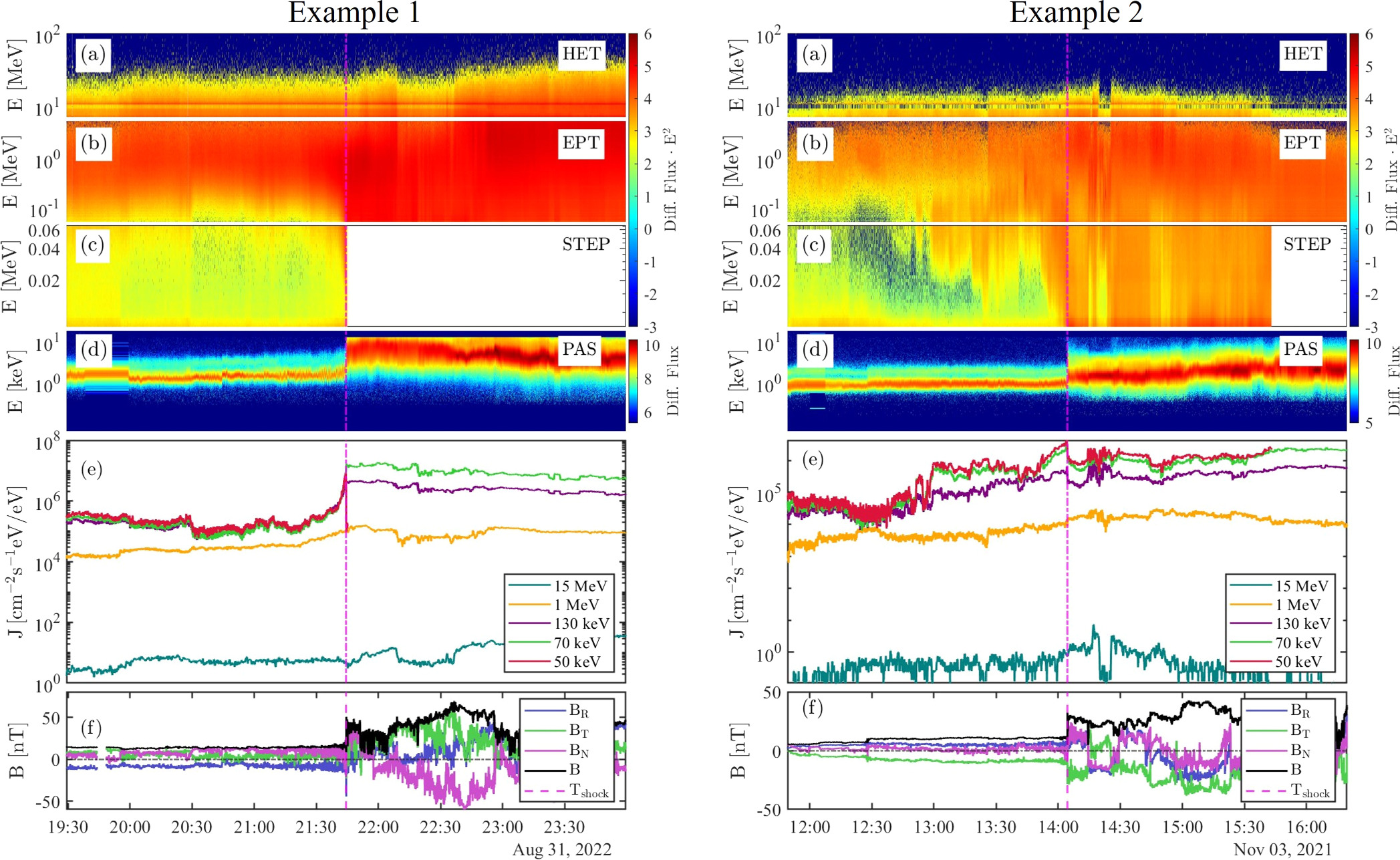
Figure 7. Refer to the following caption and surrounding text. — **Figure 7.** Two examples of energetic protons Solar Orbiter observations in response to an IP shock passage. (a)–(c) Spectrograms of energetic ions differential fluxes (in E² · cm⁻² s⁻¹sr⁻¹MeV) as measured by EPD's Sun-directed HET (a) and EPT (b) sensors, and by the STEP sensor (c). (d) Energy flux (in cm⁻²s⁻¹eV) measured by SWA-PAS. (e) Ion differential fluxes for selected energy channels. (f) Magnetic field magnitude and components.
Download figure:
Standard image High-resolution image

In both cases, the shocks are propagating through an already enhanced energetic proton population, due to a previous phase of the event or to a previous SEP event. In Figure 7 Example 1, we observe energetic protons’ differential fluxes up to 1 MeV rising exponentially upstream up to the shock crossing and then becoming constant downstream. Such time–energy profiles can be interpreted as a signature of diffusive shock acceleration (DSA; e.g., W. I. Axford et al. 1977; R. D. Blandford & J. P. Ostriker 1978; A. R. Bell 1978) operating at the IP shock. Such observation is compatible with the shock parameters measured locally, indicating a quasi-parallel (θ_Bn ∼ 22°), fast (V_sh ∼ 1100 km s⁻¹ shock with high Mach numbers (M_A ∼ M_fms ∼ 5.4). For 15 MeV particles, a more complex behavior is observed, with an irregular response to the shock passage. This can be put in the context of the highly variable environment observed in the shock downstream, with magnetic structures modulating energetic particle fluxes, with a weaker effect of the shock at affecting the behavior of these high energies. It may be noted that the 15 MeV intensity peaks downstream of the shock, which may be an essential region for further particle acceleration, as shown as well by the recent observation of strong IP shocks (see D. Lario et al. 2003; E. Kilpua et al. 2023).

The theme of complexity concerning energetic particle production is even more evident in Figure 7 Example 2, where another strong shock is shown. While the standard collection of averaging windows used for the SERPENTINE shock list yields a θ_Bnof 51° and moderate Mach numbers (M_A ∼ 3; M_fms2.3), we note that shock parameter estimation is particularly challenging in this event, due to strong disturbances in the magnetic field reported upstream/downstream of the shock, as reported in D. Trotta et al. (2023a). Such complexity yields irregular time profiles of energetic particles, where many different mechanisms of production of suprathermal and high-energy protons have been found by recent studies (L. Yang et al. 2024). Once again, in Example 2, the particle flux at the highest energy reported (15 MeV) peaks downstream of the shock, highlighting the importance of the preexisting features where IP shocks propagate.

As intensity–time profiles of energetic particles yield invaluable information about particle acceleration and transport at IP shocks, we characterized them for the Solar Orbiter sample. We study the energetic ions fluxes for the selected energy channels of 50 keV, 70 keV, 130 keV, 1 MeV, and 15 MeV (all in the spacecraft rest frame), thus employing EPD–STEP for the 50 keV response, EPD–EPT Sun for the 70 keV, 130 keV and 1 MeV response, and EPD–HET Sun for the 15 MeV channel. The profiles are visually characterized as “spike,” “plateau,” “structured/irregular,” and “no response,” summarized in the sketch reported in Figure 8. This effort continues earlier surveys of shocks at 1 au in previous solar cycles (e.g., D. Lario et al. 2003), making our study particularly relevant due to the novel energy-time resolution capabilities provided by the Solar Orbiter EPD suite and the fact that a poorly investigated range of heliocentric distances can be explored.

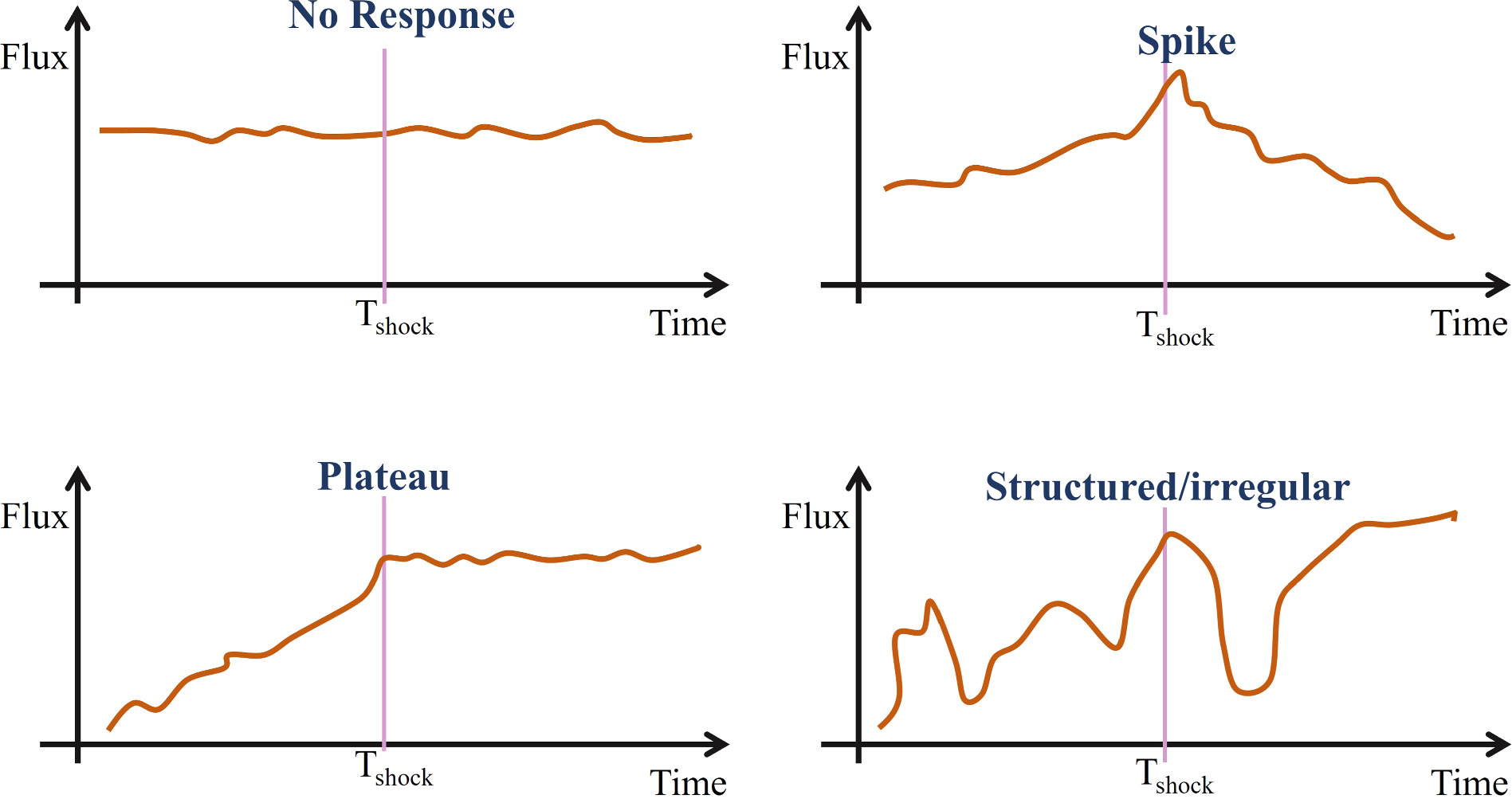
Figure 8. Refer to the following caption and surrounding text. — **Figure 8.** Sketch of the type of energetic particle flux responses to the IP shock passage.
Download figure:
Standard image High-resolution image

The outcome of our analysis is shown in Figure 9, showing a bar chart characterizing energetic particle response to the IP shock passage for the selected energy channels. The colors were chosen as follows: teal indicates “zero flux,” meaning no energetic particles were detected in the interval surrounding the shock. Then, yellow, purple, green, and red indicate the “no response,” “irregular,” “spike,” and “plateau” responses outlined in Figure 8. The “no response” case is different from the zero flux one as it has a significant flux but no changes in particle fluxes are detected in relation to the shock crossing. Note that, in Figure 9, the 50 keV bar is shorter since EPD–STEP data is available for fewer shocks than EPT and HET, with 64 shocks participating in the analysis for STEP and 79 for EPD and HET. In our data set, 88.5% of the shocks did not show a significant response at the highest selected proton energy channel (15 MeV), while 9% of them showed an irregular response. 2.5% of shocks in the sample have a spike response in the 15 MeV channel, and none show a plateau-like response. For 72% of the shock, we have no associated energetic protons (both the zero flux and no response cases) in the 1 MeV channel, 13% of them have an irregular response, 9% have a spike, and 6% have a plateau response. 130 keV particle flux enhancements are found more easily at the observed shocks, with only 41% of them not having a response. In this channel, 30% of the shocks have irregular responses, 18% of them have a spike response, and 11% are associated with a plateau response. At the lowest energies studies with EPT (70 keV), 30% of shocks were not associated with energetic protons intensity enhancements, and 31%, 24%, and 14% are associated with irregular, spike, and plateau responses, respectively. Finally, we report on the responses for suprathermal ions with energies of 50 keV. For 36% of the sample, we did not see any enhancement in the suprathermal population, while 33%, 24%, and 6% have irregular, spike, and plateau responses, respectively. These results are compatible with the ones reported in D. Lario et al. (2003). It is important to note that it is extremely common to observe irregular responses in the production of energetic particles for all the selected channels, once again emphasizing the importance of considering the variability of the medium where shocks propagate, which can profoundly modify the mechanisms of their production and transport. The cross-correlation of the characterized profiles with shock parameters will be the object of future studies.

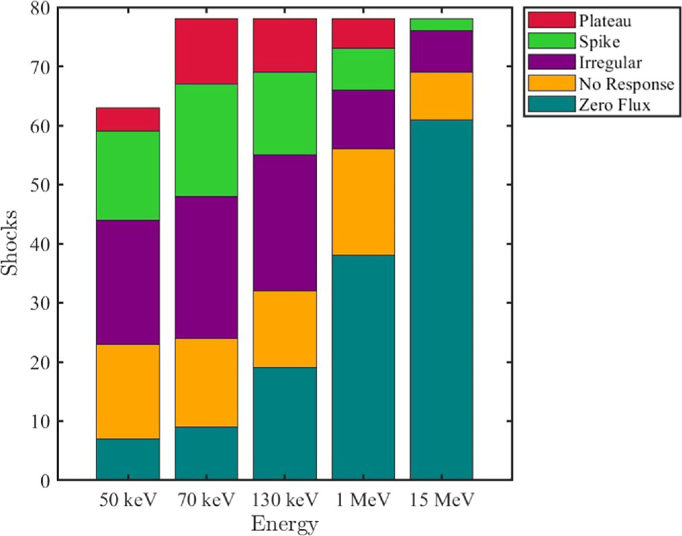
Figure 9. Refer to the following caption and surrounding text. — **Figure 9.** Bar chart describing the type of ion responses (Figure 8) at different energies for the whole IP shock sample.
Download figure:
Standard image High-resolution image

It is possible to extract further information about energetic particle production from the intensity–time profiles, by studying when particle fluxes peak relative to the shock crossing time (e.g., P. van Nes et al. 1984; D. Lario et al. 2003). From DSA theory, the time profiles are expected to peak at the same time as the shock crossing, a prediction confirmed by some observations, and failing incompatible with others (see J. Giacalone 2012; S. Perri & G. Zimbardo 2015; Y. Y. Kartavykh et al. 2016).

It is then interesting, as a further use case of the database, to report on the time difference between the peak of energetic particles and the shock passage time. This characterization is provided in the SERPENTINE shock list for the same energy channels discussed above. Figure 10 shows an overview of the time difference between the peak of energetic particle profiles and the shock crossing time for all five channels (left to right). Negative, zero, and positive values of T_peak − T_shock are the cases when the peak in particle intensity occurs before, at, and after the shock passage. In the figure, the highlighted red area corresponds to 10 minutes centered around T_p_eak − T_shock = 0, and therefore the points falling in the highlighted area have a response compatible with particle fluxes peaking at the shock (though small-scale departures are possible). Once again, Figure 10 shows how complex cases where energetic particles peak in advance/with a delay to the shock crossing time. This behavior is due to several factors, including evolutionary effects of the shocks (i.e., shock parameters making acceleration more or less favored are not constant in time), as well as spatial irregularities, where the spacecraft yields one-dimensional information sampling a complex, intrinsically three-dimensional environment. Finally, the fact that particle fluxes peaking later than the shock being more common than particles peaking in advance of the shock, suggests that particle trapping in downstream structures is important for further acceleration and for influencing particle transport properties (N. A. Schwadron et al. 2020; D. Trotta et al. 2022b; E. Kilpua et al. 2023), whereas intervening structures upstream may change this behavior (e.g., D. Lario et al. 2003).

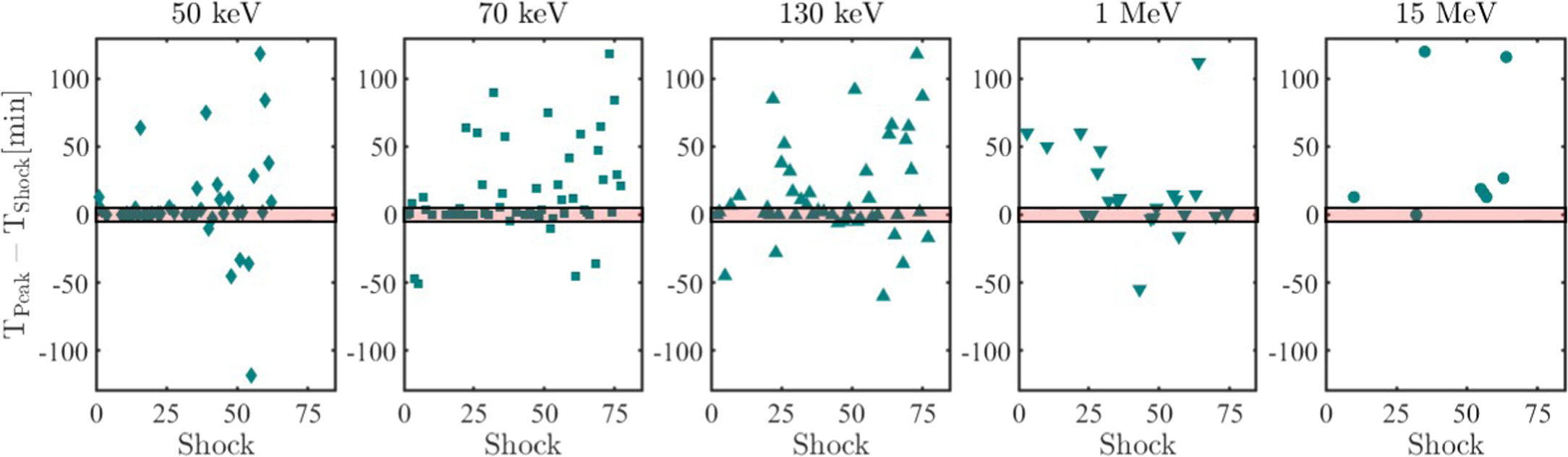
Figure 10. Refer to the following caption and surrounding text. — **Figure 10.** Time of peak vs time shock T_peak − T_shock for each event, for all the selected energy channels (left to right). The red boxes represent a 10 minute window around T_peak − T_shock = 0.
Download figure:
Standard image High-resolution image

5. Conclusions

This paper has presented an extensive in situ observational effort about IP shocks using Solar Orbiter. The importance of exploiting the Solar Orbiter data set is twofold: on the one hand, poorly explored heliocentric distances can be accessed; on the other hand, the unprecedented time-energy resolutions provided by the EPD suite open a new observational window in the study of energetic particles in the heliosphere, as shown by many recent efforts (e.g., R. F. Wimmer-Schweingruber et al. 2021; A. Kollhoff et al. 2021; D. Trotta et al. 2023b; L. Rodrìguez-Garcìa et al. 2023). This effort is in continuity with other studies using other missions and looking at IP shock statistics at different heliocentric distances (e.g., E. K. Kilpua et al. 2015; D. M. Oliveira 2023; C. A. Pérez-Alanis et al. 2023).

A sample of 100 shocks was identified using the TRUFLS detection software (Appendix A), which is publicly available and easily portable to other missions. All the shocks have been extensively characterized. The fundamental shock parameters were estimated using the publicly available SerPyShock code (D. Trotta et al. 2022a). The outcome of the analysis, including also advanced information on the shocks such as the study of wave foreshocks and energetic particle response, is the object of the SERPENTINE shock list, free to download and use through a dedicated server developed in the framework of the project (Appendix B). The SERPENTINE list employs a data processing pipeline where each shock is analyzed with the same choice of free parameters in the diagnostic procedure. In particular, the length of the upstream/downstream averaging windows has been fixed between 1 and 8 minutes. In this work, we also give the shocks’ basic parameters using a case-by-case procedure based on the visual inspection of each event, reported in Appendix C.

The general trends of Solar Orbiter IP shocks have been presented and found to be compatible with previous studies (e.g., E. K. Kilpua et al. 2015). We found that IP shocks tend to be weak, most of them have only moderate Mach numbers (≲3). The analysis of shock normal vector distributions reveals that significant departures from radial are common, an important ingredient often overlooked when modeling shock propagation in the heliosphere. The shocks’ gas and magnetic compression ratios, Alfvénic and fast magnetosonic Mach numbers, normal angles θ_Bn, and speed have been studied as a function of heliocentric distance, revealing no strong correlation with this parameter. Comparing the shock parameters measured below 0.8 au with the large sample of about 600 shocks at 1 au provided in E. K. Kilpua et al. (2015), we found that high Mach numbers are more common in the inner heliosphere. This can be due to an evolution effect of the shock drivers: at short heliocentric distances, most of the shocks are driven by CMEs, and they are faster in the early stages of their propagation (B. Vrnak et al. 2010). At short heliocentric distances, it is also easier to find quasi-parallel shocks compared to the 1 au sample, an effect due to the Parker Spiral of the heliospheric magnetic field, being less curved at low heliocentric distances (an effect discussed in J. K. Chao & Y. H. Chen 1985; D. V. Reames 1999). However, effects beyond simple drag, as well as small and large-scale disturbances of the IP magnetic field with respect to the nominal Parker spiral build a more complex picture of the typical trends of shock parameters as a function of heliocentric distance (see, for example, the scatter of shock normal vectors in RTN; Figure 2). Thus, further studies on inner heliospheric shocks will involve both future Solar Orbiter shock observations and the integration of the present survey with a similar effort using the PSP mission (see the SODA database²⁰ ).

About 50% of the shocks show enhanced wave activity, as revealed by magnetic field wavelet analyses performed on the entire shock sample. The identified wave foreshocks in frequencies between 0.01 and 1 Hz last from a few minutes to about 1 hr. Precursors at higher frequencies follow similar statistics. The analysis of the shocks’ wave environment indicates an emerging complexity in the interplay between shock-generated and preexisting magnetic fluctuations. The wave foreshocks identified are often associated with shock-reflected particles, less easily identified due to the plasma instrument's SWA-PAS instrumental limitations. Long-lasting (about 1 hr) wave/particle foreshocks have been found upstream of shocks propagating in the solar wind with low levels of magnetic field fluctuations, a result compatible with recent studies of long-lasting field-aligned beams of particles with higher energies (D. Lario et al. 2022). Interestingly, for some shocks, enhanced wave activity has been identified without particle counterparts. These, first reported by P. Kajdič et al. (2012), will be the object of future studies.

In this work, we also gave an overview of the novel capabilities of the Solar Orbiter EPD suite, yielding detailed information about energetic particle behavior at shocks and often showing complexity in particle production, beyond simple acceleration models (L. Yang et al. 2024; D. Trotta et al. 2023b). Energetic protons’ time–intensity profiles and their response to the passage of IP shocks were characterized for five different energy channels (15 MeV, 1 MeV, 130 keV, 70 keV, and 50 keV). About 70% of the shocks were found to be associated with 50 keV proton intensity increases. In contrast, 15 MeV particles were associated with 10% of the shocks showing all irregular responses, i.e., there were no plateau cases at these high energies that are considered as DSA-like responses. We note that many shocks have irregular/complex particle responses for all the energy channels, highlighting how the ambient fluctuations and shock irregularities shape particle production and transport features. Peak times of energetic particles have also been studied relative to the shock crossing times, revealing that particles may often peak earlier/later than the time the shock crosses the spacecraft. This is another effect beyond the classical picture of particle acceleration at shocks. This study is complementary to previous surveys of shock-accelerated particles (D. Lario et al. 2003), and in future studies, will be put in the context of the variability found in particle time–intensity profiles using a multimission approach (M. Neugebauer et al. 2006). In future work, the correspondence between energetic particles’ response and resonant wavelength magnetic field fluctuations, a fundamental ingredient of shock acceleration theories, will be investigated, building on earlier work done with other missions and for a narrower range of energies (M. Desai et al. 2012).

Acknowledgments

This study has received funding from the European Union's Horizon 2020 research and innovation program under grant agreement No. 101004159 (SERPENTINE, https://serpentine-h2020.eu/). Views and opinions expressed are, however, those of the authors only and do not necessarily reflect those of the European Union or the European Research Council Executive Agency. Neither the European Union nor the granting authority can be held responsible for them. This work was supported by the UK Science and Technology Facilities Council (STFC) grant ST/W001071/1. Solar Orbiter magnetometer operations are funded by the UK Space Agency (grant ST/X002098/1). Solar Orbiter is a space mission of international collaboration between ESA and NASA, operated by ESA. Solar Orbiter SWA data are derived from scientific sensors that have been designed and created and are operated under funding provided in numerous contracts from the UK Space Agency (UKSA), the UK STFC), the Agenzia Spaziale Italiana (ASI), the Centre National d'Etudes Spatiales (CNES, France), the Centre National de la Recherche Scientifique (CNRS, France), the Czech contribution to the ESA PRODEX program and NASA. Solar Orbiter SWA work at UCL/MSSL is currently funded under STFC grants ST/W001004/1 and ST/X/002152/1. EPD on Solar Orbiter is supported by the Spanish Ministerio de Ciencia, Innovación y Universidades FEDER/MCIU/AEI Projects ESP2017-88436-R and PID2019-104863RB-I00/AEI/10.13039/501100011033 and the German space agency (DLR) under grant 50OT2002. X.B.C. acknowledges DGAPA PAPIIT grant IN106724 and CONAHCyT grant CBF2023-2024-852 H.H. is supported by the Royal Society University Research Fellowship URF R1 180671. N.D. is grateful for the support from the Academy of Finland (SHOCKSEE, grant No. 346902). T.S.H. is supported by STFC grant ST/W001071/1.

Appendix A: The TRUFLS Shock Identification Algorithm

The TRUFLS code is built to look at long time series and identify shocks automatically. An important, similar effort has been made for other missions in the Heliospheric Shock Database generated and maintained at the University of Helsinki.²¹ To compile such a catalog, the authors used either visual inspection of magnetic field and plasma data, or, for a small number of missions, a machine learning algorithm (InterPlanetary Support Vector Machine).²² Once a shock candidate was identified through one of the two methods, the authors required a set of upstream/downstream relations on the magnetic field plasma data to be satisfied in order to confirm that the candidate was indeed a shock.

TRUFLS, instead, looks at where such jump conditions are satisfied using a moving average scanning the entire time series that is required to analyze. The conditions to be satisfied to identify a shock event are the following:

Here, the subscripts u and d indicate upstream and downstream averages respectively, and B and V denote the magnetic field magnitude and spacecraft frame plasma flow speed, respectively. Equations (A1) and (A2) represent the compression of the magnetic field and plasma density expected at the shock, respectively. The criterion on the plasma bulk flow speed for the FF and FR cases are summarized in Equations (A3) and (A4), respectively. We restrict our analyses to fast shocks (i.e., shocks for which the shock speed is larger than the upstream fast magnetosonic speed). Vice versa, slow shocks are not treated here. It is worth underlining that in the database,²³ a further constraint is requested to confirm that the candidate event is indeed a shock, namely, the proton temperature jump T_d/T_u≥ 1.2. Within our identification, we relax this request, due to the fact that temperature data are the ones with the highest levels of noise.

The TRUFLS code searches for times where Equations (A1)–(A4) are verified in time series containing magnetic field and plasma data. Upstream and downstream averaging windows (and an exclusion zone where the shock itself will be) are chosen, with their length being a user-defined parameter. The output of the code consists of the times when the jump conditions are satisfied, which therefore constitute the shock candidates. The process by which TRUFLS operates is further elucidated in Figure 11, where a sketch of an FF shock signature is reproduced together with the sliding averaging windows.

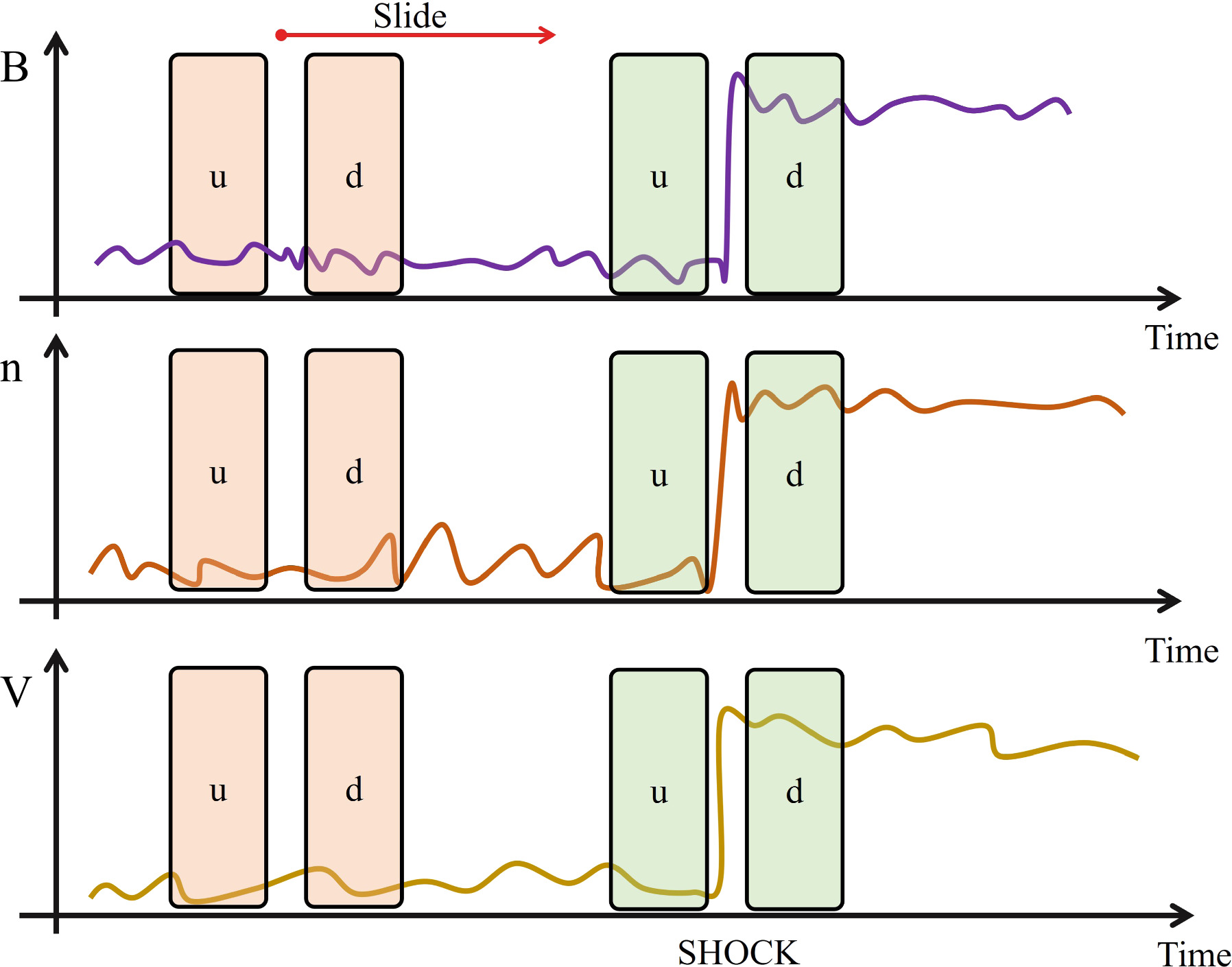
Figure 11. Refer to the following caption and surrounding text. — **Figure 11.** Sketch showing the sliding average windows (u and d, shaded panels) identifying an FF shock (green) as done in the TRUFLS code.
Download figure:
Standard image High-resolution image

It is worth underlining that when plasma data is not available, such diagnostics become more complex. While we developed a TRUFLS version working on magnetic field-only candidates that flag a lot of false positives, as Equation (A1) is easily satisfied also at structures that are not shocks. For this reason, to automatically identify shocks, we strongly recommend using both plasma and magnetic field data.

The TRUFLS distribution is publicly available on GitHub²⁴ and it may be used to identify new Solar Orbiter shocks with the most recent data set, as well as on data sets from other missions.

Appendix B: The Solar Orbiter Shock List in the SERPENTINE Data Center

The Solar Orbiter shock catalog presented here has been produced and developed as part of the SERPENTINE project. SERPENTINE targeted three main scientific questions, namely:

1.
What are the primary causes for widespread SEP events observed in the heliosphere?
2.
What are the shock acceleration mechanisms responsible for accelerating ions from thermal/suprathermal energies to near-relativistic energies in the corona and in the IP medium?
3.
What is the role of shocks in electron acceleration in large gradual and widespread events? How does it relate to ion acceleration and what is its importance relative to flare acceleration?

Scientific closure of Q1–Q3 has been targeted through comprehensive analyses, both case studies and statistical investigations, of historical and current SEP measurements and solar context observations (A. Kollhoff et al. 2021; N. Dresing et al. 2022, 2023; D. Trotta et al. 2022b; L. Rodrìguez-Garcìa et al. 2023a, 2023b; A. Afanasiev et al. 2023; N. Wijsen et al. 2023; I. C. Jebaraj et al. 2023a, 2023b; A. Dimmock et al. 2023; C. Y. Lorfing et al. 2023; N. Talebpour Sheshvan et al. 2023; E. Kilpua et al. 2023; D. Trotta et al. 2023b, 2023c, 2024a, 2024b; H. Hietala et al. 2024; I. C. Jebaraj et al. 2024; O. Pezzi et al. 2024; W. Wei et al. 2024; L. Y. Khoo et al. 2024; D. E. Morosan et al. 2024; S. Nyberg et al. 2024).

Crucially, SERPENTINE has produced and delivered a very large public release of diverse data analysis tools (A. Kouloumvakos et al. 2022; C. Palmroos et al. 2022; D. J. Price et al. 2022; D. Trotta et al. 2022a; J. Gieseler et al. 2023; A. Kouloumvakos et al. 2023) and catalogs of SEP events, IP shocks, and CMEs for historical and solar cycle 25 events. The tools and catalogs were built for easy access and are released in the hope of broad use by the heliophysics community. Altogether, five catalogs, two based on Helios data and three based on modern observations, have been released through the project data server.²⁵ Here, we focused on the in situ Cycle 25 shocks of Solar Orbiter, citable in the present version (D. Trotta et al. 2024c) through Zenodo at doi:10.5281/zenodo.12518015. The list contains all the information listed in Table 1 as well as quick-look plots and links to the SEP catalog of SERPENTINE (N. Dresing et al. 2024a). An example of how to access and use the shock list is shown in Figure 12, where the main page displaying events in the catalog is shown on the left. By clicking on each event, it is possible to access advanced information (spacecraft configuration, quick-look plots, etc.), as shown by the panel on the right. Further information, like quick-look plots of the wave environment and energetic particle response, may be accessed by clicking on the relevant sections.

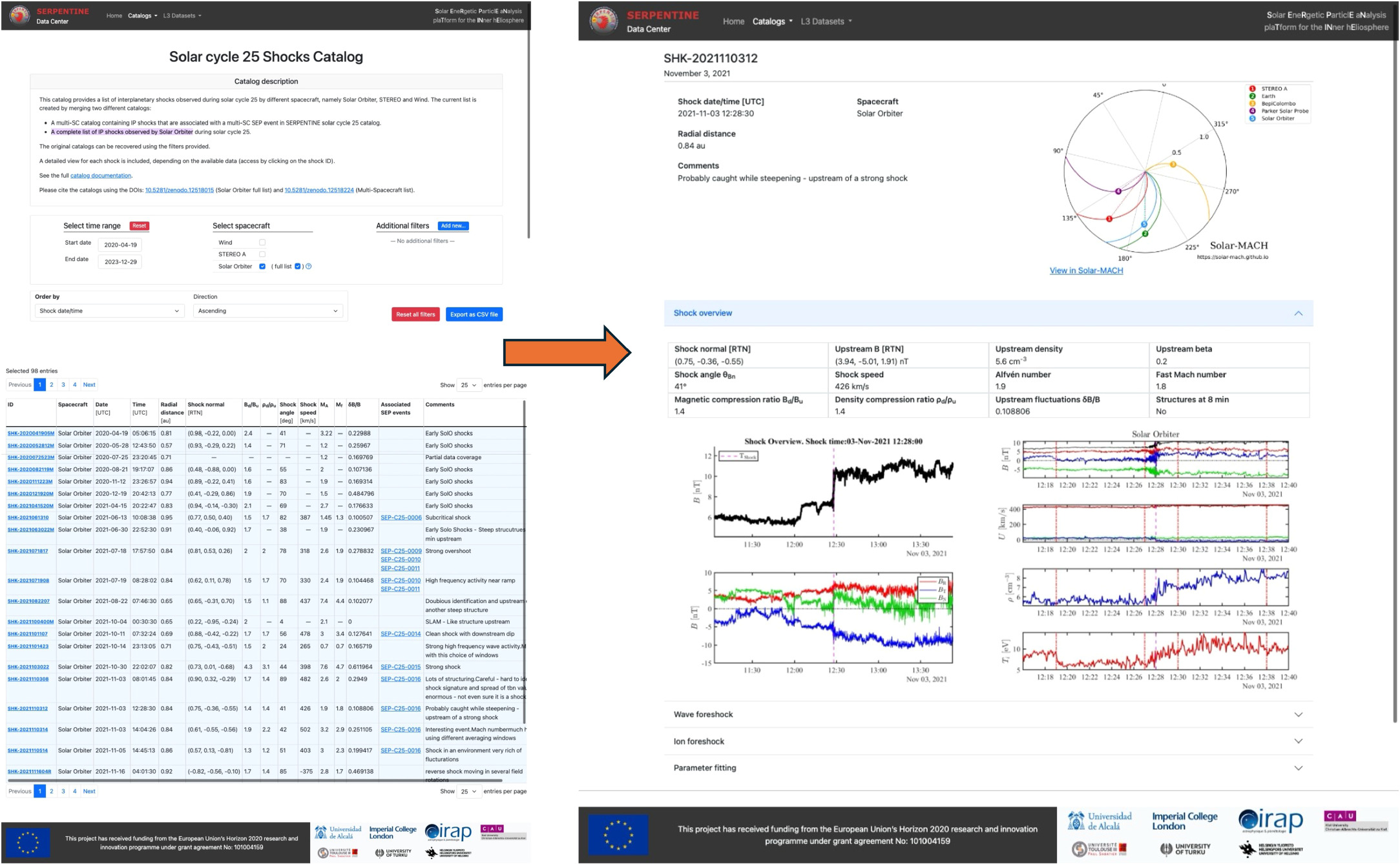
Figure 12. Refer to the following caption and surrounding text. — **Figure 12.** Screenshots of the cycle 25 Solar Orbiter shock list in the SERPENTINE data center (left), with advanced information and quick-look plots on one example event (right). Available at https://data.serpentine-h2020.eu/catalogs/sep-sc25/.
Download figure:
Standard image High-resolution image

Appendix C: Case-by-case Shock Parameters Estimation through Visual Inspection

The Solar Orbiter shock list was also inspected case by case with a semiautomated approach is adopted. First, the IP shocks are identified automatically, using the same approach as the Heliospheric Shock Database generated and maintained at the University of Helsinki.²⁶ This provides a list of IP shock candidates, and the following procedure is applied.

1.
Inspect each candidate and remove events where the field and plasma parameter changes are inconsistent with fast mode IP shocks (fast or reverse). Most misidentifications are current sheets or other complex structures.
2.
Merge windows when the same shock is identified multiple times to create a larger window that extends from upstream to downstream.
3.
For each candidate, the upstream and downstream regions are inspected to find the most reliable windows to compute shock parameters. We select the regions closest to the shock front that do not contain significant field rotations or changes in plasma moments.
4.
Shock parameters are computed using mean averages of the upstream windows. The shock normal uses the mixed-mode coplanarity method, and the shock speed is computed according to mass flux conservation.
5.
Parameters are checked to see if they are reasonable considering the structure of the shock. For example, a shock with θ_B_n ∼ 90° would not be expected to exhibit a foreshock.

It is worth noting that some additional shocks existed in this database when the automatic identification was not possible, for example, early in the mission when no ion moments were available due to the operation of the SWA-PAS instrument. These shocks were identified by looking for clear shock signatures (ramp, foot, overshoot, compression) in the MAG data and electron density calibrated from the spacecraft potential. This final database is freely available (A. Dimmock 2024).

Footnotes

Please wait… references are loading.