Abstract
We present the ancillary data and basic physical measurements for the galaxies in the ALMA Large Program to Investigate C+ at Early Times (ALPINE) survey—the first large multiwavelength survey that aims at characterizing the gas and dust properties of 118 main-sequence galaxies at redshifts 4.4 < z < 5.9 via the measurement of [ ] emission at
  (64% at >3.5σ) and the surrounding far-infrared continuum in conjunction with a wealth of optical and near-infrared data. We outline in detail the spectroscopic data and selection of the galaxies as well as the ground- and space-based imaging products. In addition, we provide several basic measurements including stellar masses, star formation rates (SFR), rest-frame ultra-violet (UV) luminosities, UV continuum slopes (β), and absorption line redshifts, as well as Hα emission derived from Spitzer colors. We find that the ALPINE sample is representative of the 4 < z < 6 galaxy population selected by photometric methods and only slightly biased toward bluer colors (Δβ ∼ 0.2). Using [
 ] as tracer of the systemic redshift (confirmed for one galaxy at z = 4.5 out of 118 for which we obtained optical [
 ]λ3727Å emission), we confirm redshifted Lyα emission and blueshifted absorption lines similar to findings at lower redshifts. By stacking the rest-frame UV spectra in the [
 ] rest frame, we find that the absorption lines in galaxies with high specific SFR are more blueshifted, which could be indicative of stronger winds and outflows.
1. Introduction
1.1. The Early Growth Phase in Galaxy Evolution
Galaxy evolution undergoes several important phases such as the ionization of neutral Hydrogen at redshifts z > 6 (also known as the Epoch of Reionizaton) as well as a time of highest cosmic star formation rate (SFR) density at z ∼ 2–3. The transition phase at z = 4–6 (a time roughly 0.9 to 1.5 billion years after the Big Bang), often referred to as the early growth phase, is currently in focus of many studies. This time is of great interest for understanding galaxy evolution as it connects primordial galaxy formation during the epoch of reionization with mature galaxy growth at and after the peak of cosmic SFR density. During a time of only 600 Myr, the cosmic stellar mass density in the universe increased by one order of magnitude (Caputi et al. 2011; Davidzon et al. 2017), galaxies underwent a critical morphological transformation to build up their disk and bulge structures (Gnedin et al. 1999; Bournaud et al. 2007; Agertz et al. 2009), and their interstellar medium (ISM) became enriched with metal from sub-solar to solar amounts (Ando et al. 2007; Faisst et al. 2016b), while at the same time the dust attenuation of the UV light significantly increased (Finkelstein et al. 2012; Bouwens et al. 2015; Fudamoto et al. 2017; Popping et al. 2017; Cullen et al. 2018; Ma et al. 2019; Yamanaka & Yamada 2019). Furthermore, the most massive of these galaxies may become the first quiescent galaxies already at z > 4 (Glazebrook et al. 2017; Tanaka et al. 2019; Faisst et al. 2019; Stockmann et al. 2020; Valentino et al. 2020). All of this put together, makes the early growth phase an important puzzle piece to be studied in order to decipher how galaxies formed and evolved to become the galaxies (either star-forming or quiescent) that we observe in the local universe.
It is evident from studies at lower redshift that multiwavelength observations are crucial for us to be able to form a coherent picture of galaxy evolution. To capture several important properties of galaxies, a panchromatic survey must comprise several spectroscopic and imaging data sets that cover a large fraction of the wavelength range of a galaxy’s light emission, including (i) the rest-frame ultra-violet (UV) containing Lyα emission, as well as several absorption lines to study stellar winds and metallicity (Heckman et al. 1997; Maraston et al. 2009; Steidel et al. 2010; Faisst et al. 2016b), (ii) the rest-frame optical containing tracers of age (Balmer break) as well as important emission lines (e.g., Hα) to quantify the star formation and gas metal properties (Kennicutt 1998; Kewley & Ellison 2008), and (iii) the far-infrared (FIR) continuum and several FIR emission lines (e.g,. [ ]
]  or [
or [ ]
]  ) that provide insights into the gas and dust properties of galaxies (De Looze et al. 2014; Pavesi et al. 2019).
Fortunately, the early growth phase at redshifts z = 4–6 is at the same time the highest-redshift epoch at which, using current technologies, such a panchromatic study can be carried out. The rest-frame UV part of the energy distribution at these redshifts has been probed in the past thanks to several large spectroscopic (Le Fèvre et al. 2015; Hasinger et al. 2018) and imaging (Capak et al. 2007; McCracken et al. 2012; Aihara et al. 2019) surveys from the ground as well as imaging surveys with the Hubble Space Telescope (HST; Scoville et al. 2007a; Grogin et al. 2011; Koekemoer et al. 2011). In addition, Hα has been accessed successfully through observations with the Spitzer Space Telescope (Stark et al. 2013; de Barros et al. 2014; Smit et al. 2014; Faisst et al. 2016b, 2019; Rasappu et al. 2016; Smit et al. 2016; Lam et al. 2019). However, the FIR of z > 4 galaxies has only been probed sparsely in the past in less than a dozen galaxies using the Atacama Large (Sub-) Millimeter Array (ALMA; Riechers et al. 2014; Capak et al. 2015; Watson et al. 2015; Willott et al. 2015; Strandet et al. 2017; Carniani et al. 2018; Zavala et al. 2018b, 2018a; Casey et al. 2019; Jin et al. 2019) as well as some as part of Herschel surveys in lensed and unlensed fields (e.g., Egami et al. 2010; Casey et al. 2012, 2014; Combes et al. 2012). Commonly targeted by observations with ALMA is singly ionized Carbon (C+) at  , which is an important coolant for the gas in galaxies and is therefore broadly related to star formation activity and gas masses (Stacey et al. 1991; Carilli & Walter 2013; De Looze et al. 2014). The [
 ] emission line is one of the strongest in the FIR and is in addition conveniently located in the ALMA Band 7 at redshifts z = 4–6 at one of the highest atmospheric transmissions compared to other FIR lines (see, e.g., Faisst et al. 2017). The origin of [
 ] emission is still debated. In addition to photodissociation regions (PDRs) and the cold neutral medium, a significant fraction can also origin from ionized gas regions or CO-dark molecular clouds (Pineda et al. 2013; Vallini et al. 2015; Pavesi et al. 2016). Also, the increasing temperature of the Cosmic Microwave Background has an effect on the relation between [
 ] and star formation (Ferrara et al. 2019). Both potentially complicates the interpretation of [
 ] as SFR indicator at high redshifts. Similar to Hα, [
 ] traces the gas kinematics in a galaxy and is therefore an important component to quantify rotation- and dispersion-dominated systems as well as outflows (Jones et al. 2017; Pavesi et al. 2018; Kohandel et al. 2019; Ginolfi et al. 2020).
The FIR landscape has dramatically changed with the completion of the ALMA Large Program to Investigate C+ at Early Times (ALPINE; #2017.1.00428.L). ALPINE is laying the ground work for the exploration of gas and dust properties in 118 main-sequence star-forming galaxies in the early growth phase at 4.4 < z < 5.9 and herewith started the first panchromatic survey of its kind at these redshifts (Figure 1).
1.2. ALPINE in a Nutshell
In the following, we summarize the scope of the ALPINE survey, we refer to Le Fèvre et al. (2019) for a broader overview of the program. ALPINE is a 69 hr large ALMA program started in Cycle 5 in 2018 May and completed during Cycle 6 in 2019 February. In total, 118 galaxies have been observed in Band 7 (covering [ ] emission at
  and its nearby continuum) at a spatial resolution of <1
0 and with integration times ∼30 minutes on-source depending on their predicted [
 ] flux. The galaxies originate from two fields, namely the Cosmic Evolution Survey field (COSMOS; 105 galaxies, Scoville et al. 2007b) and the Extended Chandra Deep Field South (ECDFS; 13 galaxies, Giacconi et al. 2002). Due to gaps in the transition through the atmosphere, the galaxies are split into two different redshift ranges spanning 4.40 < z < 4.65 and 5.05 < z < 5.90 with medians of
  and 5.5 and galaxy numbers of 67 and 51, respectively. All galaxies are spectroscopically confirmed by either Lyα emission or rest-UV absorption lines and are selected to be brighter than an absolute UV magnitude of M1500 = −20.2. This limit is roughly equivalent to an SFR cut at
  and corresponds roughly to a limiting luminosity in [
 ] emission of
 ![${L}_{[{\rm{C}}{\rm{I}}{\rm{I}}]}={1.2}_{-0.9}^{+1.9}\times {10}^{8}\,{L}_{\odot }$](https://content.cld.iop.org/journals/0067-0049/247/2/61/revision1/apjsab7ccdieqn22.gif) (assuming the relation derived by De Looze et al. 2014). Assuming a 3.5σ detection limit, the [
(assuming the relation derived by De Looze et al. 2014). Assuming a 3.5σ detection limit, the [ ] detection rate is 64%, and continuum emission is detected in 19% of the galaxies (see Figure 2).
The main science goals enabled by ALPINE are diverse and cover many crucial research topics at high redshifts:
- 1.Connecting [
 ] to star formation at high redshifts,
 - 2.Coherent study of the total SFR density at z > 4 including the contribution of dust-obscured star formation,
- 3.Study of gas dynamics and merger statistics from [] kinematics and quantification of UV-faint companion galaxies,
- 4.Study of gas fractions and dust properties at z > 4,
- 5.The first characterization of ISM properties using and []/FIR continuum diagnostics for a large sample at z > 4,
- 6.Quantifying outflows and feedback processes in z > 4 galaxies from [] line profiles.


Note that ALPINE provides at the same time the equivalent of a blind-survey of approximately 25 square-arcminutes. This enables us to estimate the obscured fraction of star formation (mostly below z = 4) by finding UV-faint galaxies with FIR continuum or [ ] emission. The serendipitous continuum sources and [
 ] detections are discussed in detail in Bethermin et al. (2020) and F. Loiacono et al. (2020, in preparation). A more detailed description of these science goals can be found in our survey overview paper (Le Fèvre et al. 2019).
ALPINE is based on a rich set of ancillary data, which makes it the first panchromatic survey at these high redshifts including imaging and spectroscopic observations at FIR wavelengths (see Figure 1). The backbone for a successful selection of galaxies are rest-frame UV spectroscopic observations from the Keck telescope in Hawaii as well as the European Very Large Telescope (VLT) in Chile. These are complemented by ground-based imaging observations from rest-frame UV to optical, HST observations in the rest-frame UV, and Spitzer coverage above the Balmer break at rest-frame  . The latter is crucial for the robust measurement of stellar masses at these redshifts (e.g., Faisst et al. 2016a).
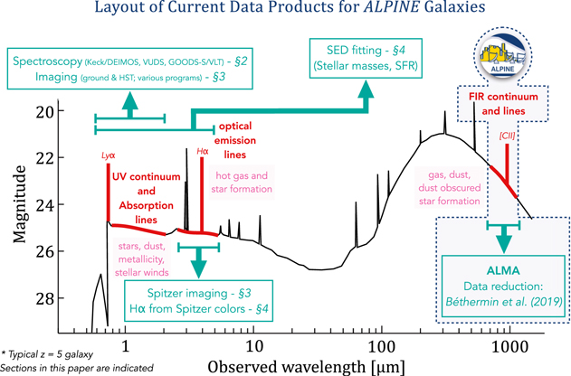
Figure 1. ALPINE builds the corner stone of a panchromatic survey at z = 4–6. The diagram shows the multiwavelength data products that are currently available for all of the ALPINE galaxies. The currently covered parts of the spectrum are indicated in red. The numbers link to sections in this paper where the data products and their analysis are explained in detail. The spectrum sketch is based on a typical z = 5 galaxy (adapted from Harikane et al. 2018).
Download figure:
Standard image High-resolution image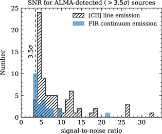
Figure 2. Signal-to-noise ratio of the ALMA-detected sources in the ALPINE sample. The different histograms show the numbers for [ ] and continuum detections above 3.5σ. For more information, see Le Fèvre et al. (2019) and Bethermin et al. (2020).
Download figure:
Standard image High-resolution imageFor a survey overview of ALPINE see Le Fèvre et al. (2019) and for details on the data analysis see Bethermin et al. (2020). In this paper, we present these valuable ancillary data products and detail several basic measurements for the ALPINE galaxies. The outline of the paper is sketched in Figure 1. Specifically, in Section 2, we present the spectroscopic data and detail the spectroscopic selection of the ALPINE galaxies. In the same section, we also present stacked spectra and touch on velocity offsets between Lyα, [ ], and absorption line redshifts. Section 3 is devoted to the photometric data products, which include ground- and space-based photometry. In Section 4.1, we detail the derivation of several galaxy properties from the observed photometry. These include stellar masses, SFRs, UV luminosities, UV continuum slopes, as well as Hα emission derived from Spitzer colors. We conclude and summarize in Section 5. All presented data products are available in the online printed version of this paper.28
The different catalogs and their columns are described in detail in the Appendix A. HST cutouts and rest-frame UV spectra for each of the ALPINE galaxies are shown in Appendix B.
], and absorption line redshifts. Section 3 is devoted to the photometric data products, which include ground- and space-based photometry. In Section 4.1, we detail the derivation of several galaxy properties from the observed photometry. These include stellar masses, SFRs, UV luminosities, UV continuum slopes, as well as Hα emission derived from Spitzer colors. We conclude and summarize in Section 5. All presented data products are available in the online printed version of this paper.28
The different catalogs and their columns are described in detail in the Appendix A. HST cutouts and rest-frame UV spectra for each of the ALPINE galaxies are shown in Appendix B.
Throughout the paper, we assume the ΛCDM cosmology with  , ΩΛ = 0.70, and Ωm = 0.30. All magnitudes are given in the AB system (Oke 1974) and stellar masses and SFRs are normalized to a Chabrier (2003) initial mass function (IMF).
2. Spectroscopic Data and Selection
2.1. Spectroscopic Selection of ALPINE Galaxies
The ALPINE survey is only possible due to a spectroscopic pre-selection of galaxies from large spectroscopic surveys on COSMOS and ECDFS. This is because the ALMA frequency bands are narrow ( ), and in order to observe [
 ] emission, the redshift has to be known within a precision of
  . The galaxy selection is refined to optimize the efficiency of the ALMA observations by creating groups of galaxies in spectral dimensions. Our sample also includes seven galaxies that were previously observed with ALMA by Riechers et al. (2014) and Capak et al. (2015). These are HZ1, HZ2, HZ3, HZ4, HZ5, HZ6/LBG-1, and HZ8, which correspond to the ALPINE galaxies DC_536534, DC_417567, DC_683613, DC_494057, DC_845652, DC_848185, and DC_873321, respectively. Furthermore, four galaxies from the VUDS survey (vc_5101288969, vc_5100822662, and vc_510786441 in COSMOS and ve_530029038 in ECDFS) are observed twice (resulting in a total number of 122 observations). The duplicate observations are used for quality assessment. Bethermin et al. (2020) describes the combination of these observations.
The rest-frame UV spectroscopic data from which the ALPINE sample is selected combine various large surveys on the COSMOS and ECDFS fields. Out of the 105 ALPINE galaxies on the COSMOS field, 84 are obtained by the large DEIMOS spectroscopic survey (Capak et al. 2004; Mallery et al. 2012; Hasinger et al. 2018) at the Keck telescope in Hawaii. The remaining spectra on the COSMOS field are obtained from the VIMOS Ultra Deep Survey (VUDS; Le Fèvre et al. 2015; Tasca et al. 2017) at the VLT in Chile. In total, six of the VUDS spectra are independently also observed as part of the Keck/DEIMOS survey (vc_5100559223, vc_5100822662, vc_5101218326, vc_5101244930, vc_5101288969, vc_510786441). The redshifts are consistent within  , and we do not find any systematic offsets between the two observations (see also Section 2.4.1). Out of the 13 galaxies in the ECDFS field, 11 are obtained from spectroscopic observations with VIMOS (9) and FORS2 (229
) at the VLT (Vanzella et al. 2007, 2008; Balestra et al. 2010), and two come from the HST grism survey GRAPES (Malhotra et al. 2005; Rhoads et al. 2009). The spectral resolution of the different data set varies between R ∼ 100 (ECDFS/GRAPES grism), R ∼ 180 (ECDFS/VIMOS), R ∼ 230 (COSMOS/VUDS), R ∼ 660 (ECDFS/FORS2), and R ∼ 2500 (COSMOS/DEIMOS).
, and we do not find any systematic offsets between the two observations (see also Section 2.4.1). Out of the 13 galaxies in the ECDFS field, 11 are obtained from spectroscopic observations with VIMOS (9) and FORS2 (229
) at the VLT (Vanzella et al. 2007, 2008; Balestra et al. 2010), and two come from the HST grism survey GRAPES (Malhotra et al. 2005; Rhoads et al. 2009). The spectral resolution of the different data set varies between R ∼ 100 (ECDFS/GRAPES grism), R ∼ 180 (ECDFS/VIMOS), R ∼ 230 (COSMOS/VUDS), R ∼ 660 (ECDFS/FORS2), and R ∼ 2500 (COSMOS/DEIMOS).
Biases toward dust-poor star-forming galaxies with strong rest-frame UV emission lines (such as Lyα) can be common in purely spectroscopically selected samples. To minimized such biases as much as possible, the spectroscopically observed galaxies have been pre-selected through a variety of different selection methods. The largest fraction of galaxies in ALPINE is drawn from the Keck/DEIMOS and VUDS surveys on the COSMOS field. Both surveys include galaxies pre-selected in various ways, resulting in the most representative and inclusive spectroscopic high-redshift galaxy sample. Specifically, the VUDS survey combines predominantly a photometric redshift selection with a color-selected Lyman Break Galaxy (LBG) selection (Le Fèvre et al. 2015), known as the Lyman-break drop-out technique (see, e.g., Steidel et al. 1996; Dickinson 1998). The Keck/DEIMOS survey (providing 71% of the total ALPINE sample) consists of galaxies that are selected by narrowband surveys at z ∼ 4.5 (7%) and z ∼ 5.7 (27%), the drop-out technique (color selection) over the whole redshift range (49%), as well as purely by photometric redshifts (11%). In addition, four galaxies are selected by a 4.5 μm excess and one galaxy was pre-selected through X-ray emission using the Chandra Observatory. On the ECDFS field, the galaxies are mostly color-selected. Table 1 summarizes the different selections and corresponding numbers of galaxies and provides a complete list of references. We also list the numbers of galaxies with Lyα emission (76%) and weak Lyα emission or Lyα absorption (∼24%). Note that the Keck/DEIMOS and VUDS samples have similar Lyα emission properties. However, note that above z = 5, the ALPINE sample is strongly dominated by narrowband-selected galaxies.
Table 1. Spectroscopy and Selection of ALPINE Galaxies
| Survey | Selection | Number | Ref. |
|---|---|---|---|
| COSMOS field (105 galaxies) | |||
| Keck/DEIMOSa | 84 | 1 | |
| narrowband (z ∼ 4.5)c | 6 | ||
| narrowband (z ∼ 5.7)d | 23 | ||
| LBG (color)e | 41 | ||
| pure photo-zf | 9 | ||
 excess excess |
4 | ||
| X-ray (Chandra) | 1 | ||
| with Lyα emission | 66 | ||
| weak Lyα emission or absorption | 18 | ||
| VUDS | 21 | 2 | |
| photo-z + LBG | 21 | ||
| [narrowband (z ∼ 4.5) | 3]b | ||
| [narrowband (z ∼ 5.7) | 1]b | ||
| [LBG (color) | 1]b | ||
 excess excess |
1]b | ||
| with Lyα emission | 16 | ||
| weak Lyα emission or absorption | 5 | ||
| ECDFS field (13 galaxies) | |||
| VLT GOODS-S | 11 | 3 | |
| primarily LBG (color) | 11 | ||
| total with Lyα emission | 6 | ||
| total without Lyα emission | 5 | ||
| HST/GRAPES | 2 | 4 | |
| Grism (no a priori selection) | 2 | ||
| with Lyα emission | 2 | ||
| weak Lyα emission or absorption | 0 | ||
Notes.
aFor a detailed description of the selection criteria, we refer the reader to Mallery et al. (2012) and Hasinger et al. (2018). bSix of these galaxies are also observed as part of the Keck/DEIMOS survey (ref. 1). The corresponding number per selection from the Keck/DEIMOS program is given in square-brackets for those six galaxies. cLyα emitters selected with NB711. dLyα emitters selected with NB814. eColor-selected galaxies in B, g+, V, r+, and z++ using the criteria from Ouchi et al. (2004), Capak et al. (2004, 2011), Iwata et al. (2003), Hildebrandt et al. (2009). fGalaxies with a photometric redshift z > 4 with a probability of > 50% based on the Ilbert et al. (2010) photo-z catalog.References: (1) Capak et al. (2004), Mallery et al. (2012), Hasinger et al. (2018), (2) Le Fèvre et al. (2015), (3) Vanzella et al. (2007, 2008), Balestra et al. (2010), (4) Malhotra et al. (2005), Rhoads et al. (2009).
Download table as: ASCIITypeset image
Figure 3 shows the distribution of redshifts of the ALPINE galaxies in the COSMOS and ECDFS fields. The colored histogram bars show stacked numbers of galaxies that are pre-selected by the different methods discussed above. The bins with galaxies in the ECDFS field are hatched. The narrowband-selected galaxies are prominent at z ∼ 5.7 and represent the largest fraction of galaxies at z > 5 in ALPINE. On the other hand, the z < 5 sample consists mostly of color-selected galaxies. The VUDS galaxies are most represented at z < 5, while the DEIMOS spectra and the galaxies in ECDFS cover the whole redshift range.
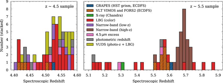
Figure 3. Redshift distribution of ALPINE galaxies. Each bar shows the stacked number of different selections per bin (see Table 1 and description in text). The bins with galaxies from the ECDFS field are hatched. The left and right panels show galaxies in the two different redshift bins.
Download figure:
Standard image High-resolution imageFigure 4 shows the distribution of observed magnitudes as well as rest-frame 1500 Å and  luminosity of galaxies selected by the different methods. The photometry that is used is explained in detail in Section 3. The 1500 Å rest-frame luminosity is derived from spectral energy distribution (SED) fitting (see Section 4.2 for details). The 4000 Å rest-frame luminosity is derived directly from the UltraVISTA Ks and VLT Ksv magnitude for galaxies in the COSMOS and GOODS-S field, respectively. The magnitudes and luminosities are not corrected for dust attenuation. Note that the K-band is rest-frame 3000 Å at the highest redshifts (z = 5.9); hence at these redshifts, older and dustier galaxies would be biased to lower luminosities. As expected for spectroscopically selected galaxies, the ALPINE sample covers the brighter part of the galaxy magnitude and luminosity distribution. The different selection methods on their own are distributed differently in this parameter space. Most noticeably, the z ∼ 5.7 narrowband-selected galaxies reside at the faintest luminosities, while the 4.5 μm continuum excess selected galaxies are among the brightest. The Chandra X-Ray Observatory–detected galaxy DC_845652 (green star) at z = 5.3 outshines all of the galaxies in UV luminosity.
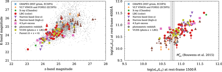
Figure 4. Comparison of observed (i.e., not corrected for dust) z-band and K-band magnitudes (left panel) and luminosities (right panel) for different selections listed in Table 1. The measurements on the parent sample in COSMOS at 4 < z < 6 is shown in light gray. The color-coding is the same as in Figure 3. The arrows show 1σ upper limits. The gray area denotes the  , the knee of the UV luminosity function, which corresponds to −21.1 ± 0.15 (or
  ) at z = 5 (Bouwens et al. 2015). The derivation of the photometry is described in detail in Section 3.
Download figure:
Standard image High-resolution imageAll in all, although naturally biased to the brightest galaxies, this diverse selection function makes ALPINE an exemplary panchromatic survey that enables the study of a representative high-z galaxy sample at UV, optical, and FIR wavelengths.
2.2. Uniform Calibration of Spectra
All of the rest-frame UV spectra discussed in Section 2.1 are relative-flux corrected to remove sensitivity variations across the spectrograph as well as to correct atmospheric absorption features. However, not all of the spectra have been absolute-flux calibrated, which is important to measure absolute quantities such as their Lyα emission. Hence, we recalibrate the spectra using the Galactic extinction-corrected total broad-, intermediate-, and narrowband photometry of the ALPINE galaxies (see Section 3 for details on the photometry). It turns out that the absolute-flux calibrated spectra are in excellent agreement (within better than 5% in flux) with our measured photometry, and the recalibration is not necessary in these cases. As the spectra come from different surveys, we convert them to a common format during the recalibration procedure.
To perform the absolute-flux calibration, we convolve each of the spectra with the transmission functions of the various optical broad-, intermediate-, and narrowband filters that exist on the COSMOS and ECDFS fields, respectively. On average, we use 4–9 filters for galaxies at z < 5 and 2–4 at z > 5. If the filter extends further than the spectrum, we extrapolate the spectrum by its medium continuum value. If the filter extends significantly beyond the spectrum (>50%), we do not consider the filter. We then compare the photometry obtained from the spectra to the total and Galactic extinction-corrected photometry discussed in Section 3, which allows us to obtain an average correction factor for each spectrum. We found that a single number for this correction per galaxy is enough for the calibration as the spectra already have been relative-flux calibrated. Since the uncalibrated spectra are mostly in units of counts, this correction is on the order of 10−21 for most galaxies. Our recalibration corrects for slit-losses and seeing variations. We also scale the variance in order to conserve the signal-to-noise ratio (S/N) of the spectrum. The final precision of our calibration is around 5%–10% in flux, which corresponds to the 1σ uncertainty in the photometry. Note that we do not consider undetected spectroscopic fluxes in this procedure; however, we use the constraints gained from the upper limits in the photometry for the calibration. Figure 5 shows three absolute-calibrated spectra at z ∼ 4.53, z ∼ 4.56 (with weak Lyα), and z ∼ 5.68 to visualize our method. The filters that were used for the calibration are indicated in colors.
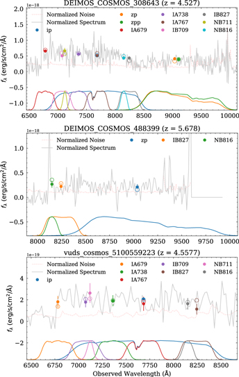
Figure 5. Absolute calibration of rest-frame UV spectra. Shown are three examples at z = 4.53, z = 4.56, and z = 5.68. The spectra are convolved by the filters, and the photometry (open circles) is compared to the total and Galactic extinction-corrected broad-, intermediate-, and narrowband photometry from catalogs (filled circles) described in Section 3.
Download figure:
Standard image High-resolution image2.3. Stacked Spectra: Overview over Rest-frame UV Emission and Absorption Lines in ALPINE Galaxies
Figures 6 and 7 show stacks of different spectra. In order to create median-stacks of the spectra, we resample the spectra to a common wavelength grid and stack them in rest frame using their respective redshifts derived from [ ] or, if not available, from rest-UV absorption lines or Lyα emission. All stacks are subsequently binned to a resolution of 2 Å for visual purposes to emphasize the UV absorption features. To obtain a per-pixel uncertainty from the sky background for each stack (visualize by the gray line), we simply combine the inverse variances in the individual spectra in quadrature. The latter are the original inverse variance that we adjusted to the new normalization described in Section 2.2.
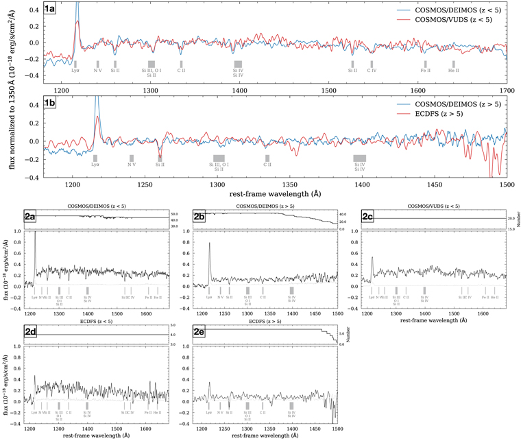
Figure 6. Examples of stacked ALPINE spectra. Panels 1a and 1b show stacked spectra at z < 5 (in COSMOS from DEIMOS observations and as part of the VUDS survey) and z > 5 (on COSMOS from DEIMOS and on ECDFS from VIMOS and FORS2 observations), respectively. The stacks are all normalized to the continuum between  and
and  and common emission and absorption features are indicated with gray bars. Note that the VUDS spectra have a lower native resolution (R ∼ 230) compared to the DEIMOS observations (R ∼ 2500); therefore, the latter have been degraded in resolution using a 1D Gaussian window function for visual comparison. Panels 2a through 2e show stacks at z < 5 and z > 5 for the different data sets. The number of spectra included per wavelength is shown on the top of each panel. The uncertainty in flux is indicated by the light gray line. The y-axis scale is the same such that the continuum brightness can be compared.
Download figure:
Standard image High-resolution imagePanels 1a and 1b of Figure 6 compare the full stacked spectra of galaxies at z < 5 in COSMOS from observations with DEIMOS and as part of VUDS, as well as at z > 5 from observations in COSMOS from DEIMOS and in ECDFS from VIMOS and FORS2. In the former case, we adjust the resolution of the DEIMOS spectra (R ∼ 2500) to that of the VUDS observations (R ∼ 230) by applying a 1D Gaussian smoothing. The spectra are normalized to the median flux in the rest-frame wavelength range between 1300 and 1400 Å before stacking. For stacks of galaxies at z > 5, the rest-frame wavelength reaches up to 1500 Å, while for lower-redshift stacks, we show wavelengths up to rest frame 1700 Å. Several prominent spectral features are visible in the stacks in both redshift bins (indicated by gray bars). These include the Lyα emission line and  at 1241 Å and in addition UV absorption lines such as
  at 1260 Å, the
  -[
-[ ]-
]- complex at 1301 Å, the two
  lines at 1398 Å, as well as
  ,
,  , and
, and  at 1527 Å, 1548 Å, and 1640 Å, respectively. Furthermore, we see indication of
  absorption at 1608 Å in the COSMOS/DEIMOS spectra stack at z < 5. The depth of the UV absorption features are comparable for the different observations with the different instruments, verifying similar quality and little biases. However, note that the features in the ECDFS spectra are less pronounced due to the factor ∼6 smaller number of spectra contributing to the stacks compared to the DEIMOS stacks. Panels 2a through 2e show the stacks for variously selected data sets below and above z = 5. The spectra are not normalized before stacking in these cases to provide a comparison of the absolute-flux values for the different redshifts and samples to the reader. The number of spectra per wavelength are shown on the top right for each panel. Note again that the number of high-redshift spectra drops toward redder wavelengths. This has to be kept in mind when analyzing the spectral features in the stacks. Emission and absorption lines are indicated as in the other panels. As expected, the stacked spectra at higher redshifts are fainter, but still significant UV absorption features are present (see also Faisst et al. 2016b; Khusanova et al. 2019; Pahl et al. 2020).
Figure 7 shows stacked spectra in COSMOS observed with DEIMOS for the different selection categories (see also Table 1 and Figure 3). We split the LBG category in galaxies below and above z = 5. All of the spectra are smoothed with a Savitzky–Golay filter with size of 2 Å for visualization purposes. The total number of spectra per stack is indicated in the upper left corner. All panels are scaled the same way to emphasize differences in brightness. The X-ray detected galaxy at z = 5.3 is UV bright compared to the other stacks and shows strong  emission with overlaid
  absorption as well as broad
  emission. LBGs (i.e., color-selected galaxies) are preferentially fainter but of similar continuum brightness as narrowband-selected galaxies at z ∼ 4.5. The latter show significant
  ,
,  , and
, and  absorption. As expected, narrowband-selected galaxies at z ∼ 5.7 show strong Lyα emission and a faint continuum such that the S/N is too low to detect UV absorption features at great significance. The stack of galaxies selected by photometric redshifts shows to first-order similar properties as the LBGs. The 4.5 μm-excess continuum selected galaxies are, on average, the continuum brightest galaxies and show significant Lyα emission as well as absorption features.
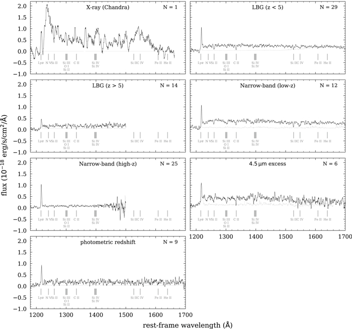
Figure 7. Stacked spectra in COSMOS for each of the selections discussed in Section 2.1 and listed in Table 1. Emission and absorption features are indicated by gray bars, and the number of spectra in the stack is shown on the upper right corner. We also show the X-ray-detected galaxy (DC_845652) at z = 5.3, which shows strong and broad  and
and  emission. The uncertainty in flux is indicated by the light gray line.
Download figure:
Standard image High-resolution image2.4. Rest-UV Emission and Absorption Lines and Velocity Offsets
2.4.1. Measurements
We measure basic quantities from the individual rest-frame UV spectra. These include the redshift and equivalent width of Lyα emission as well as redshifts from various absorption lines.
The Lyα redshift ( ) is based on the peak of the (asymmetric) Lyα emission to allow a direct comparison with models of Lyα radiative transfer (see, e.g., Hashimoto et al. 2015). The Lyα flux is measured by fitting a Gaussian to the line and for measuring the equivalent width (
 ) the continuum redward of the Lyα line is used. These measurements are explained in more detail in Cassata et al. (2020).
The absorption redshifts are measured for each individual spectrum, if possible, using the lines  (
( ), [
), [ ] (
] ( ),30
),30
 (1334.5 Å),
  (1393.8 Å) and
  (1402.8 Å),
  (1526.7 Å), and
  (1549.5 Å).31
The first four are covered by observations in all galaxies, while the coverage of the latter depends on the redshift of the galaxy. Note that some of the above lines are predominantly formed in the ISM (low-ionization interstellar [IS] lines;
(1549.5 Å).31
The first four are covered by observations in all galaxies, while the coverage of the latter depends on the redshift of the galaxy. Note that some of the above lines are predominantly formed in the ISM (low-ionization interstellar [IS] lines;  , [
, [ ],
],  ,
,  ), while others are formed in stellar winds (high-ionization wind lines;
  or
or  ) and therefore can display strong velocity shifts (e.g., Castor & Lamers 1979; Leitherer et al. 2011). To increase the S/N of our measurements, we use all of the above lines to derive an absorption line redshift (referred to as
  ), but we compare the individual redshift from the IS (
 ) and wind (
 ) lines to investigate potential systematic differences. Before performing any measurements, we subtract a continuum model from each individual spectrum. The model is derived by fitting a fourth-order polynomial to the spectrum, which is smoothed by a 5 Å box kernel. We then fit the above absorption lines in five different rest-frame wavelength windows [1240 Å, 1280 Å], [1280 Å, 1320 Å], [1320 Å, 1350 Å], [1370 Å, 1420 Å], and [1500 Å, 1570 Å]. For the separate fit of the IS and wind lines, we split the last window into two ranges, namely [1510 Å, 1540 Å] and [1530 Å, 1570 Å] to separate the IS line
  and the wind line
  , respectively. The absorption lines can be significantly asymmetric due to stellar winds and the effect of optical depth. Fitting a single Gaussian to them could therefore bias the redshift measurements. Instead, we use the stacked spectrum of LBGs at z ∼ 3 from Shapley et al. (2006) as a template, which we cross-correlate to the observed data within the wavelength range of a given window by χ2 minimization. We let the redshift vary within a velocity range of
  (corresponding to roughly 0.01 in redshift) around a prior absorption redshift, which is obtained by a manual cross-correlation of the same template to all possible absorption lines at once using the interacting redshift-fitting tool SpecPro32
(Masters & Capak 2011). We found that this approach significantly removes degeneracies in the fit and at the same time allows a visual inspection of all of the spectra to flag the ones with low S/N where no reasonable fit can be obtained.33
For each galaxy, the so obtained χ2(z) distribution is then converted into a probability density function p(z) for each of the windows. These are combined, by choosing the necessary absorption lines, to a total probability P(z) from which the final absorption line redshifts (
(corresponding to roughly 0.01 in redshift) around a prior absorption redshift, which is obtained by a manual cross-correlation of the same template to all possible absorption lines at once using the interacting redshift-fitting tool SpecPro32
(Masters & Capak 2011). We found that this approach significantly removes degeneracies in the fit and at the same time allows a visual inspection of all of the spectra to flag the ones with low S/N where no reasonable fit can be obtained.33
For each galaxy, the so obtained χ2(z) distribution is then converted into a probability density function p(z) for each of the windows. These are combined, by choosing the necessary absorption lines, to a total probability P(z) from which the final absorption line redshifts ( ,
,  , or
, or  ) are derived. The errors on these redshifts are derived by repeating this measurement 200 times, thereby perturbing the fluxes according to a Gaussian error distribution with σ defined by the average flux noise of the continuum. Typical uncertainties are on the order of
  .
.
As mentioned in Section 2.1, six galaxies in COSMOS have been observed by the Keck/DEIMOS and VUDS spectroscopic surveys. Therefore there are two measurements for each of these galaxies. Specifically, for vc_5100559223, vc_5100822662, vc_5101218326, and vc_5101244930, the IS+wind redshift measurements agree within  ,
,  ,
,  , and
, and  . These values are on the order of the measurement uncertainties. Note that while the VUDS slits are oriented east–west, the DEIMOS slits can be oriented north–south or in any other angle. This different orientation could also be responsible for the differences in velocity offsets. On the other hand, for vc_5101288969 and vc_510786441, we find significant differences of
  and
and  . A close inspection of the spectra shows that these are very low in S/N. Also, both have low visual quality flags (−99 and 1, indicating not robust measurements are possible), and their redshifts are fit with less than three lines; thus, they should not be trusted. For all six spectra, we decided to prefer the VUDS observations because of their slightly better S/N at a cost of lower resolution.
2.4.2. Velocity Offsets with Respect to [C ii] FIR Redshifts
The detection of [ ] by ALMA provides the systemic redshift of a galaxy. This enables us to study velocity offsets of rest-frame UV absorption lines and Lyα emission that will inform further about the properties of the ISM in these galaxies similarly to studies at lower redshifts using Hα and
  ]
]  (e.g., Steidel et al. 2010; Marchi et al. 2019). Here, we give an overview of the velocity properties and compare them for galaxies with high and low specific SFRs.
In the following, we define the velocity difference for two redshifts (z1 and z2) as  where
where  . The measurement of the [
 ] redshifts are detailed in Bethermin et al. (2020). They are defined as the peak of a Gaussian fit to the [
 ] line with spectral resolution of
  . The uncertainty of the redshift measurements was estimated by a Monte Carlo simulations with perturbed fluxes according to the error per spectral bin. The average uncertainty is roughly
  . For the absorption lines, we require that
  is measured from at least three absorption lines, and we only show galaxies that have not been flagged by our visual inspection with SpecPro as unreliable (flag −99). The average intrinsic measurement error per galaxy is
  . In relation to that, a systematic uncertainty of
  in the rest-frame wavelength of the absorption lines (e.g,. due to calibration issues) turns into a velocity shift of
  .
.
Figure 8 shows stacked histograms of velocity differences. The number of galaxies used as well as the median of the distribution with scatter (not error on the median) are indicated as well. The upper panel compares the velocities measured from Lyα and the IS+wind absorption lines. We find a median offset on the order of  , which is consistent with other measurements at the same redshifts (see, e.g., Faisst et al. 2016b; Pahl et al. 2020) as well as at z ∼ 2−3 (Steidel et al. 2010). The center and bottom panels compare the IS+wind and Lyα redshifts to the systemic redshift (here defined as the [
 ]
]  redshift, Bethermin et al. 2020). For the former, we find an offset of
  , and for the latter, we find
  . These negative and positive velocity offsets can be related in a simple physical model involving the resonant scattering of Lyα photons and outflowing gas in the outskirts of galaxies (see detailed discussion in Steidel et al. 2010). The redshifted Lyα emission line (with respect to systemic) can be explained by resonant scattering of the Lyα photons. Preferentially, redshifted Lyα photons scattered from the back of the galaxy can make it unscattered through the intervening gas inside the galaxy along the line of sight. The blueshift of IS absorption may depend on the outflow velocity of the absorbing gas as well as its covering fraction (or optical depth) inside the galaxy along the line of sight toward the observer. For a more in-depth discussion, we refer the reader to a companion paper by Cassata et al. (2020). Overall, we do not see a significant dependence of the velocity differences on the various selection techniques (color-coded in the figure).
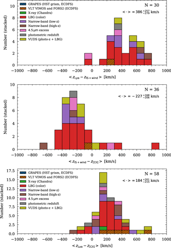
Figure 8. Stacked histograms of velocity offsets between redshifts derived from different spectral features. The number of galaxies and median of the distribution (including scatter) are indicated. Shown are the velocity offsets between Lyα emission and IS+wind absorption lines (top panel), as well as between Lyα, IS+wind, and systemic redshift (middle and bottom panel). The latter two are discussed in detail in a forthcoming paper (Cassata et al. 2020). The average errors are on the order of  , which corresponds to the size of the bins. We do not find any significant biases introduced by the different selection methods (color-coded as in previous figures).
Download figure:
Standard image High-resolution imageFigure 9 compares the velocity offsets between IS ( , [
, [ ],
],  ,
,  ) and wind (
 ,
,  ) lines. We require that at least three IS lines and one wind line is measured. In addition, only galaxies that pass our visual classification (i.e., have flags other than −99, see above) are used. Overall, we do not see any statistical difference between IS and wind lines, although there is a tail toward higher blueshifts in the case of wind lines. However, wind and outflows may be increased in galaxies with high and spatially dense star formation and young stellar populations. Therefore, we would expect different velocity shifts for the absorption lines with respect to the systemic redshift for highly star-forming galaxies. In Figure 10, we investigate this picture by stacking galaxies at the extreme ends of the sSFR distribution (we refer to Section 4 for details on the measurement of the physical properties of our galaxies), namely low (
 ) and high (
 ) sSFR, in their corresponding rest-frames defined by the systemic redshift (i.e., [
 ]
]  redshift). The sSFR is a good proxy of the star formation density in a galaxy as well as the age of the current stellar population (see, e.g., Cowie et al. 2011). We show the stacked spectra in five wavelength regions covering prominent absorption lines for each sSFR bin. The vertical dashed lines show the different absorption lines in the [
 ] rest frame. First, we verify that the shifts between IS and wind lines are very similar for each sSFR bin (in concordance with Figure 8). However, it is intriguing that in the low sSFR stack, all absorption lines agree well with the [
 ] redshift, while in the high sSFR stack, the lines are significantly blueshifted by
  . We also note that in the high sSFR stack, the
  line shows a noticeable P-Cygni profile indicative of strong winds and outflows (Castor & Lamers 1979). These findings fit well into a picture of strong winds and outflows produced by the high star formation in these galaxies, which is also in line with recent results obtained through the stacking of ALPINE [
 ] spectra (Ginolfi et al. 2020).
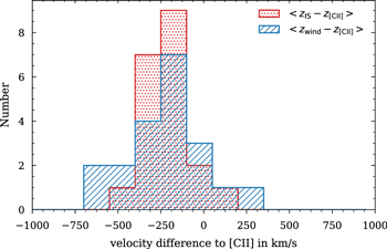
Figure 9. Histogram of velocity offset with respect to systemic (defined by the [ ]
]  redshift) for IS (red; [
 ],
],  , and
, and  ) and stellar wind affected absorption lines (blue;
  and
and  ). The average errors are on the order of ∼200 km s−1, which corresponds to the size of the bins.
Download figure:
Standard image High-resolution image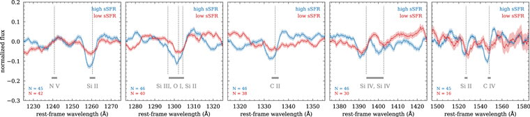
Figure 10. Stacked spectra (in  systemic redshift) in two bins of sSFR (red:
  , blue:
  ) for five wavelength regions covering prominent rest-UV absorption lines. The derivation of the sSFR for the ALPINE galaxies is detailed in Section 4.1. The average number of spectra in each bin is indicated together with the prominent absorption and emission lines. We note systematically stronger blueshifts of all absorption lines for the high sSFR stack. Particularly, note the strong blueshift of the high-ionization wind lines. The
  lines in the high sSFR bin also show indication of a more pronounced P-Cygni profile, indicative of strong stellar winds and outflows in high sSFR galaxies. The 1σ uncertainties of the stacked spectra is indicated by the shaded regions.
Download figure:
Standard image High-resolution image2.4.3. How Well Does [C ii] Trace Systemic Redshift? Comparison to Optical [O ii] Emission
The extended nature of [ ] may be indicative of its origin in the diffuse interstellar medium in addition to PDRs (Stacey et al. 1991; Gullberg et al. 2015; Vallini et al. 2015; Faisst et al. 2017). Moreover, recent work by Ginolfi et al. (2020) shows that [
 ] emission is significantly affected by large-scale outflows caused by a high rate of star formation in these galaxies. However, as shown by the same study, the outflows seem to be symmetric, and therefore, we do not expect them to significantly change the centroid of the [
 ] emission line.
During 2019 January 13–15, we were able to obtain a near-IR spectrum of one of our ALPINE galaxies (DC_881725 at ![${z}_{[{\rm{C}}\mathrm{II}]}=4.5777$](https://content.cld.iop.org/journals/0067-0049/247/2/61/revision1/apjsab7ccdieqn152.gif) ) using the Multi-Object Spectrometer For Infra-Red Exploration (MOSFIRE; McLean et al. 2010, 2012) at the 10 m Keck I telescope on Maunakea in Hawaii. The observations of a total on-source integration time of
) using the Multi-Object Spectrometer For Infra-Red Exploration (MOSFIRE; McLean et al. 2010, 2012) at the 10 m Keck I telescope on Maunakea in Hawaii. The observations of a total on-source integration time of  in K band (
 ) were carried out under clear weather conditions with an excellent average seeing FWHM of
  . We performed a standard data reduction using the MOSFIRE data reduction pipeline34
(Version 2018). From the produced 2D spectrum and variance map, we extract the 1D spectrum at the spatial location of the galaxy using a weighted mean across ±3.5 spatial pixels (
. We performed a standard data reduction using the MOSFIRE data reduction pipeline34
(Version 2018). From the produced 2D spectrum and variance map, we extract the 1D spectrum at the spatial location of the galaxy using a weighted mean across ±3.5 spatial pixels ( ).
).
We are able to detect the optical [ ] doublet (3727.09 Å and 3729.88 Å) at the spatial position of the galaxy at a level of >5σ. Note that this is the first detection of optical [
 ] in a galaxy with [
 ] measurement from ALMA, which allows us, for the first time, to compare these two lines at these redshifts. In the bottom panel of Figure 11, we show the final spectrum in the rest frame of the [
 ] emission. The width of ∼4 Å includes both [
 ] lines. The theoretical rest-frame wavelength of the doublet is indicated by the black arrows. The position of the line agrees perfectly with the [
 ] redshift derived from ALMA, indicating that FIR [
 ] and optical [
 ] trace the same systemic redshift. In addition, the top panel of the Figure shows the [
 ] FIR line for comparison of the central wavelength of the lines. Note that the actual width of the [
 ] line is more than 100 times larger than the the one of the optical [
 ] line.
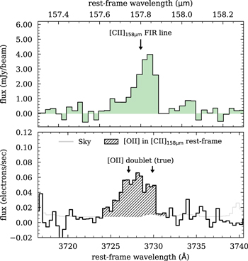
Figure 11. Comparison of optical and FIR emission lines in the case of galaxy DC_881725. Top panel: [ ] emission line at
  observed with ALMA. Bottom panel: the black line shows the optical [
 ] doublet at
  observed with the MOSFIRE spectrograph on Keck in the rest-frame of the [
 ] emission. The theoretical rest-frame wavelength of the doublet is indicate by the two arrows. This shows that there is no significant velocity offset between the [
 ] FIR and optical [
 ] emission; hence, this verifies the validity of [
 ] as tracer of the systemic redshift of this galaxy.
Download figure:
Standard image High-resolution image3. Photometry from Ground and Space
In this section, we summarize the ground- and space-based photometric data that are available for the ALPINE galaxies in the COSMOS (105 galaxies) and ECDFS (13 galaxies) fields. Although these fields differ in survey depth, reduction methods, and number and type of photometric filters used, we find that their overall photometric measurements are comparable within 1σ limits after their conversion to total magnitudes and the correction for the specific biases of each survey. Therefore, we can treat them separately to the first order for the matter of measuring various physical properties of the galaxies. The basis catalogs to which we match the ALPINE galaxies in the COSMOS and ECDFS field are the COSMOS201535 (Laigle et al. 2016) and the 3D-HST36 (Brammer et al. 2012; Skelton et al. 2014) catalog, respectively. A summary of the different data available on the two fields including filter names, wavelengths, 3σ depths, and references to the measurements are given in Tables 2 and 3, respectively. In the following, we describe these data in more detail.
Table 2. Photometry Available for Galaxies on the ECDFS Field
| Observatory/Instrument | Filter | Central λ | 3σ depth | Ref. |
|---|---|---|---|---|
| (Å) | (mag) | |||
| Ground-based | ||||
| MPG-ESO/WFI | U38 | 3633.3 | 27.3 | 1 |
| b | 4571.2 | 26.6 | 1 | |
| v | 5377.0 | 26.6 | 1 | |
| Rc | 6536.3 | 26.9 | 1 | |
| I | 9920.2 | 26.5 | 1 | |
| VLT/VIMOS | U | 3720.5 | 28.6 | 2 |
| R | 6449.7 | 27.8 | 2 | |
| VLT/ISAAC | Jv | 12492.2 | 25.6 | 3 |
| Hv | 16519.9 | 25.1 | 3 | |

|
21638.3 | 25.0 | 3 | |
| CFHT/WIRCam | Jw | 12544.6 | 25.1 | 4 |

|
21590.4 | 24.5 | 4 | |
| Subaru/Suprime-Cam | IA427 | 4263.4 | 25.7 | 5 |
| IA445 | 4456.0 | 25.7 | 5 | |
| IA505 | 5062.5 | 25.8 | 5 | |
| IA527 | 5261.1 | 26.7 | 5 | |
| IA550 | 5512.0 | 26.0 | 5 | |
| IA574 | 5764.8 | 25.7 | 5 | |
| IA598 | 6000.0 | 26.6 | 5 | |
| IA624 | 6233.1 | 26.5 | 5 | |
| IA651 | 6502.0 | 26.7 | 5 | |
| IA679 | 6781.1 | 26.6 | 5 | |
| IA738 | 7371.0 | 26.5 | 5 | |
| IA767 | 7684.9 | 25.5 | 5 | |
| IA797 | 7981.0 | 25.2 | 5 | |
| IA856 | 8566.0 | 25.0 | 5 | |
| Space-based | ||||
| HST/ACS | F435W | 4328.7 | 29.1 | 6 |
| F606W | 5924.8 | 29.1 (29.0) | 6,7 | |
| F775W | 7704.8 | 28.4 | 6 | |
| F814W | 8058.2 | 28.9 | 7 | |
| F850LP | 9181.2 | 27.9 | 6 | |
| HST/WFC3 | F125W | 12516.3 | 27.6 | 8 |
| F140W | 13969.4 | 26.7 | 9 | |
| F160W | 15391.1 | 27.7 | 8 | |
| Spitzer/IRAC | ch1 | 35634.3 | ∼26.0a | 10 |
| ch2 | 45110.1 | ∼26.0a | 10 | |
| ch3 | 57593.4 | 24.4 | 11 | |
| ch4 | 79594.9 | 24.3 | 11 | |
Note.
aThe exposure time varies between 10 and 300 ks (corresponding to roughly 1.8 in magnitudes).References: (1) Hildebrandt et al. (2006); Erben et al. (2005), (2) Nonino et al. (2009), (3) Wuyts et al. (2008); Retzlaff et al. (2010), (4) Hsieh et al. (2012), (5) Cardamone et al. (2010), (6) Giavalisco et al. (2004), (7) Koekemoer et al. (2011), (8) Grogin et al. (2011); Koekemoer et al. (2011), (9) Brammer et al. (2012); van Dokkum et al. (2013), (10) Ashby et al. (2013); Guo et al. (2013), (11) Dickinson et al. (2003).
Download table as: ASCIITypeset image
3.1. Photometry on the ECDFS Field
The photometry for the galaxies on the ECDFS field is taken directly from the 3D-HST catalog, which provides ground-based observations as well as a wealth of data from HST imaging. The photometry (total fluxes and magnitudes) is corrected for Galactic extinction, PSF size as well as other biases; therefore, no further corrections are applied. The ALPINE galaxies are matched visually to the spatially closest 3D-HST counterpart using the HST WFC3/IR F160W image as reference. The spectroscopic redshifts match the photometric redshifts within their uncertainty (∼0.1–0.2), ensuring that we identified the correct counterpart.
The ground-based photometry available in ECDFS (including references) is listed in Table 2. Summarizing, this includes the U38, b, v, Rc, and I broadband filters from the Wide Field Imager on the 2.2 meter MPG/ESO telescope, the U and R bands from VIMOS on the VLT, the near-IR filters Jv, Hv, and  from ISAAC on the VLT, Jw and
  data taken by WIRCam on the CFHT, as well as 14 intermediate-band filter from the Suprime-Cam on the Subaru telescope. For galaxies at z = 4.5 and 5.5, the Lyman-break falls roughly in the v and the Rc-band, and therefore, the galaxies are expected to be only faintly (or not at all) visible in these and blueward filters. On the other hand, the galaxies are bright at observed near-IR wavelengths, i.e., filters redward of the z band (corresponding to roughly the F850LP filter). Figure 12 shows the stacked F850LP (z), Jv (J), and
  (K) magnitude distributions of the ECDFS ALPINE galaxies split in z < 5 (hatched blue) and z > 5 (hatched red). As expected, the latter sample occupies slightly fainter magnitudes.
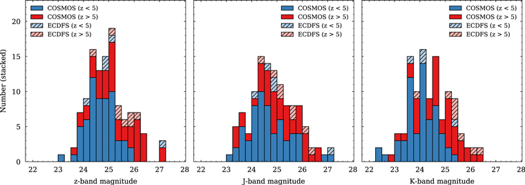
Figure 12. Stacked histograms of the magnitude distribution for the ALPINE galaxies in the COSMOS (solid) and ECDFS (hatched) fields. The blue and red color-coding indicates galaxies at z < 5 and z > 5, respectively. The magnitudes (from left to right) correspond to z++, J, and Ks bands for COSMOS and F850LP, Jv, and  bands for ECDFS (see Tables 2 and 3 for more information on the filters).
Download figure:
Standard image High-resolution imageThe space-based photometry includes the four Spitzer bands at 3.6,  ,
,  , and
, and  . In addition, the public 3D-HST catalog includes a wealth of HST photometry. Specifically, it contains measurements in the ACS bands F435W, F606W, F775W, F814W, and F850LP as well as in the WFC3/IR bands F125W, and F160W bands for all 13 ALPINE galaxies. Only 10 galaxies have measurements in the WFC3/IR band F140W. The HST photometry is measured on PSF-matched images. As described in Skelton et al. (2014), the Spitzer and ground-based photometry are measured using the MOPHONGO (Labbé et al. 2006; Wuyts et al. 2007; Whitaker et al. 2011), which uses a high-resolution image (here the HST imaging) as spatial prior to estimate the contributions from neighboring blended sources in the lower resolution image. The different depths of these observations as well as references are listed in Table 2. A query of the Barbara A. Mikulski Archive for Space Telescopes (MAST37
) using the mastquery Python package38
shows that in addition to the HST measurements contained in the 3D-HST catalog, four, ten, and two galaxies have coverage in the WFC3/IR bands F098M, F105W, and F110W, respectively. None of the galaxies has ACS F475W coverage. These additional data that are not published in the 3D-HST catalog come from various other observation programs in and around the ECDFS field. We subsequently measure this additional photometry for all ALPINE galaxies in ECDFS using SExtractor (version 2.19.5, Bertin & Arnouts 1996) in different aperture sizes (
. In addition, the public 3D-HST catalog includes a wealth of HST photometry. Specifically, it contains measurements in the ACS bands F435W, F606W, F775W, F814W, and F850LP as well as in the WFC3/IR bands F125W, and F160W bands for all 13 ALPINE galaxies. Only 10 galaxies have measurements in the WFC3/IR band F140W. The HST photometry is measured on PSF-matched images. As described in Skelton et al. (2014), the Spitzer and ground-based photometry are measured using the MOPHONGO (Labbé et al. 2006; Wuyts et al. 2007; Whitaker et al. 2011), which uses a high-resolution image (here the HST imaging) as spatial prior to estimate the contributions from neighboring blended sources in the lower resolution image. The different depths of these observations as well as references are listed in Table 2. A query of the Barbara A. Mikulski Archive for Space Telescopes (MAST37
) using the mastquery Python package38
shows that in addition to the HST measurements contained in the 3D-HST catalog, four, ten, and two galaxies have coverage in the WFC3/IR bands F098M, F105W, and F110W, respectively. None of the galaxies has ACS F475W coverage. These additional data that are not published in the 3D-HST catalog come from various other observation programs in and around the ECDFS field. We subsequently measure this additional photometry for all ALPINE galaxies in ECDFS using SExtractor (version 2.19.5, Bertin & Arnouts 1996) in different aperture sizes ( and 3″) as well as auto magnitudes. For this, we first create a mosaic of all of the HST pointings that overlap with the ALPINE galaxies using the AWS-drizzler39
tool that is part of the grizli40
Python package (G. Brammer 2020, in preparation.). We use a 0
and 3″) as well as auto magnitudes. For this, we first create a mosaic of all of the HST pointings that overlap with the ALPINE galaxies using the AWS-drizzler39
tool that is part of the grizli40
Python package (G. Brammer 2020, in preparation.). We use a 006 pixel scale and all HST images are registered to Gaia (see Section 3.3). SExtractor is run with relative THRESH_TYPE, and we set DETECT_MINAREA, DETECT_THRESH, DEBLEND_MINCONT, and DEBLEND_NTHRESH to 3, 1.5, 1.5, 0.001, and 64, respectively. If no object is detected above the threshold (1.5σ) within 0
7 (roughly the ground-based seeing) of the original ALPINE coordinates, we consider the galaxy as undetected in a given band and replace its flux by a 1σ limit that is computed from the rms noise at the position of the galaxy. The photometry measured by SExtractor is subsequently corrected for galactic foreground extinction, which we assume to be constant for all galaxies in ECDSF at
 . Figure 13 summarizes the HST data available for the galaxies in the ECDFS field. The blue squares show the layout of all of the HST pointings as of 2019 October, with darker shades of blue indicating more observations. The ALPINE galaxies at z < 5 and z > 5 are indicated with orange circles and squares, respectively.
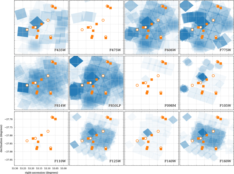
Figure 13. HST pointing footprints on the ECDFS field (blue) for different HST ACS and WFC3/IR filters. Darker colors mean more observations. The ALPINE galaxies are indicated by orange circles and squares for z < 5 and z > 5, respectively.
Download figure:
Standard image High-resolution image3.2. Photometry on the COSMOS Field
Most of the ALPINE galaxies (105 out of 118) reside in the COSMOS field, and we match them to the latest photometric measurements presented in the COSMOS2015 catalog. The matching is again done on a galaxy-by-galaxy basis using the HST/ACS F814W as well as UltraVISTA Ks images as references. We also match against the photometric redshifts given in the catalog in order to identify the correct counterpart.41
In Table 3, we list all of the photometric measurements available for the ALPINE galaxies on the COSMOS field. Summarizing, these include u*-band observations from MegaCam on CFHT, the B, V, r+, i+, z++ as well as 12 intermediate-band and two narrowband filters from the Suprime-Cam on Subaru, the YHSC-band from the Hyper Suprime-Cam on Subaru as well as near-IR bands Hw and  from WIRCam on CFHT and Y, J, H, and Ks from VIRCAM on the VISTA telescope. In addition, the galaxies are covered by the four Spitzer channels from 3.6 μm to
  from the SPLASH survey42
(Capak et al. 2012; Steinhardt et al. 2014; Laigle et al. 2016). As described in (Laigle et al. 2016), the Spitzer photometry is measured using IRACLEAN (Hsieh et al. 2012), which uses positional priors from higher-resolution imaging (in this case the zYJKHKs detection χ2-image) to deblend the photometry.
from the SPLASH survey42
(Capak et al. 2012; Steinhardt et al. 2014; Laigle et al. 2016). As described in (Laigle et al. 2016), the Spitzer photometry is measured using IRACLEAN (Hsieh et al. 2012), which uses positional priors from higher-resolution imaging (in this case the zYJKHKs detection χ2-image) to deblend the photometry.
Table 3. Photometry Available on the COSMOS Field
| Observatory/Instrument | Filter | Central λ | 3σ depth | Ref. |
|---|---|---|---|---|
| (Å) | (mag)a | |||
| Ground-based | ||||
| CFHT/MegaCam | u* | 3823.3 | 26.6 | 1 |
| Subaru/Suprime-Cam | B | 4458.3 | 27.0 | 1, 2 |
| V | 5477.8 | 26.2 | 1,2 | |
| r+ | 6288.7 | 26.5 | 1, 2 | |
| i+ | 7683.9 | 26.2 | 1, 2 | |
| z++ | 9105.7 | 25.9 | 1, 2 | |
| IA427 | 4263.4 | 25.9 | 1, 2 | |
| IA464 | 4635.1 | 25.9 | 1, 2 | |
| IA484 | 4849.2 | 25.9 | 1, 2 | |
| IA505 | 5062.5 | 25.7 | 1, 2 | |
| IA527 | 5261.1 | 26.1 | 1, 2 | |
| IA574 | 5764.8 | 25.5 | 1, 2 | |
| IA624 | 6233.1 | 25.9 | 1, 2 | |
| IA679 | 6781.1 | 25.4 | 1, 2 | |
| IA709 | 7073.6 | 25.7 | 1, 2 | |
| IA738 | 7361.6 | 25.6 | 1, 2 | |
| IA767 | 7684.9 | 25.3 | 1, 2 | |
| IA827 | 8244.5 | 25.2 | 1, 2 | |
| NB711 | 7119.9 | 25.1 | 1, 2 | |
| NB816 | 8149.4 | 25.2 | 1, 2 | |
| Subaru/HSC | YHSC | 9791.4 | 24.4 | 1 |
| CFHT/WIRCam | Hw | 16311.4 | 23.5 | 1 |

|
21590.4 | 23.4 | 1 | |
| VISTA/VIRCAM | Y | 10214.2 | 24.8 (25.3)b | 1 |
| J | 12534.6 | 24.7 (24.9)b | 1 | |
| H | 16453.4 | 24.3 (24.6)b | 1 | |
| Ks | 21539.9 | 24.0 (24.7)b | 1 | |
| Space-based | ||||
| HST/ACS | F435W | 4328.7 | −c | − |
| F475W | 4792.3 | −c | − | |
| F606W | 5924.8 | −c | − | |
| F814W | 8058.2 | 29.2 | 3 | |
| F850LP | 9181.2 | −c | − | |
| HST/WFC3 | F098M | 9877.4 | −c | − |
| F105W | 10584.9 | −c | − | |
| F110W | 11623.8 | −b | − | |
| F125Wd | 12516.3 | 27.6c,d | 4 | |
| F140W | 13969.4 | −c | − | |
| F160Wd | 15391.1 | 27.5(25.0)c,d,e | 4, 5 | |
| Spitzer/IRAC | ch1 | 35634.3 | 25.5 | 1, 6, 7 |
| ch2 | 45110.1 | 25.5 | 1, 6, 7 | |
| ch3 | 57593.4 | 23.0 | 1, 7 | |
| ch4 | 79594.9 | 22.9 | 1, 7 | |
Notes.
aDepth is measured in aperture for ground-based photometry.
bDepths of the ultra-deep area are given in parenthesis.
cAncillary pointings; therefore, depth varies depending on the specific observations.
dMost of these data come from the CANDELS survey and their depth is indicated.
eSome of the F160W data comes from the DASH survey (depth given in parenthesis).
aperture for ground-based photometry.
bDepths of the ultra-deep area are given in parenthesis.
cAncillary pointings; therefore, depth varies depending on the specific observations.
dMost of these data come from the CANDELS survey and their depth is indicated.
eSome of the F160W data comes from the DASH survey (depth given in parenthesis).
References: (1) see Laigle et al. (2016), (2) Taniguchi et al. (2007, 2015) (3) Scoville et al. (2007b), Koekemoer et al. (2007), (4) Grogin et al. (2011), Koekemoer et al. (2011), (5) Momcheva et al. (2017), (6) Capak et al. (2012), Steinhardt et al. (2014), (7) Sanders et al. (2007).
Download table as: ASCIITypeset image
Contrary to the 3D-HST photometry catalog, the fluxes and magnitudes in the COSMOS2015 catalog are not total and not corrected for systematic biases and Galactic extinction. To perform these corrections, we follow the steps outlined in the appendix of Laigle et al. (2016). Specifically, we use the 3″ diameter aperture magnitudes ( ), which we correct for photometric (oi, see their Equation (4)) and systematic offsets (sf, see their Table 3) by applying

where i is the object identifier and f denotes the different filters. The total magnitudes are subsequently corrected for Galactic extinction by applying

where  is the Galactic extinction from the Schlegel et al. (1998) maps on COSMOS for each object as given in the catalog and Ff are the extinction factors per filter given in Table 3 of Laigle et al. (2016).
Figure 12 shows the stacked magnitude distribution in  (z), J, and Ks (K) bands for the z < 5 (blue) and z > 5 (red) sub-samples. As expected, the high-redshift galaxies are fainter in all bands. In addition, we find the magnitude distributions between the galaxies in ECDFS and COSMOS to be similar. This indicates no major discrepancies in photometric (and, hence, physical) properties between the two samples.
In terms of HST imaging, all galaxies except one are observed in ACS F814W (Koekemoer et al. 2007; Scoville et al. 2007a). In addition to this, a MAST search shows that several galaxies are covered by other observing programs in the ACS bands F435W (3), F475W (5), F606W (21), and F850LP (5) as well as in the WFC3/IR bands, F105W (11), F110W (5), F125W (16), F140W (13), and F160W (53).43 Note that the observations in F160W primarily come from the CANDELS survey (covering the central part of COSMOS; Grogin et al. 2011; Koekemoer et al. 2011) as well as the “drift and shift” (DASH; Momcheva et al. 2017) survey. While the CANDELS imaging is deep (>27.5 magnitudes at 3σ), the data from the DASH survey is much shallower (25.0 magnitudes at 3σ), and therefore, only half of the galaxies are detected. Furthermore, the spatial sampling in the latter does not allow for a detailed study of the structure of the galaxies. Figure 14 summarizes the HST pointings on the COSMOS field (blue). The CANDELS area in the center of the COSMOS field as well as the three DASH stripes are evident. The locations of the ALPINE galaxies are indicated with circles (z < 5) and squares (z > 5). The photometry available is summarized in Table 3 including depths (where applicable) and references.
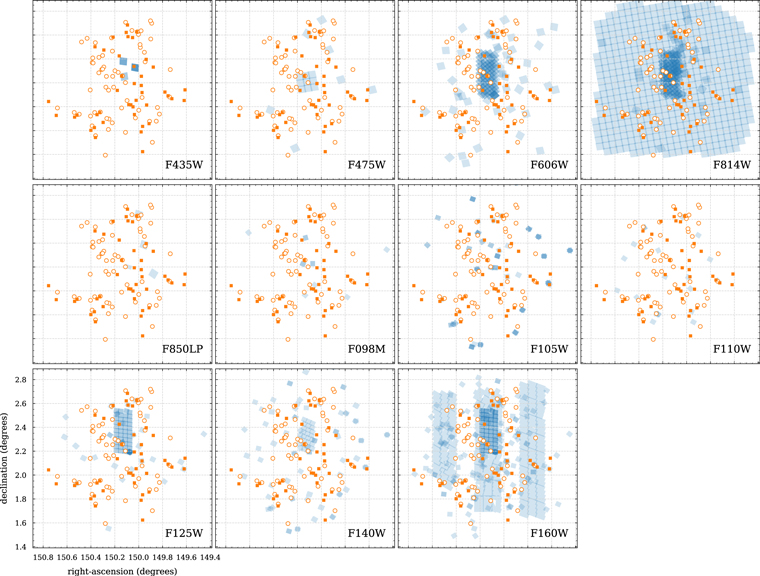
Figure 14. HST pointing footprints on the COSMOS field (blue) for different HST ACS and WFC3/IR filters. Darker colors mean more observations. The ALPINE galaxies are indicated by orange circles and squares for z < 5 and z > 5, respectively.
Download figure:
Standard image High-resolution imageIn order to measure the photometry in these HST bands, we use SExtractor in the same way as described in Section 3.1. We first create a mosaic (006 pixel sizes and registered to Gaia) using the AWS-drizzler. We subsequently measure the HST photometry of on each of the images for all ALPINE galaxies with coverage using SExtractor in apertures (0
7 and 3″) as well as auto magnitudes. If no object is detected above the set threshold level within 0
7 of the original ALPINE coordinates, we consider the galaxy as undetected in a given band. Similar to Equation (2), we correct the HST photometry for galactic foreground extinction using the Schlegel et al. (1998) extinction map. We compare these measurements to the ground-based photometry, by first performing a PSF matching by smoothing the original HST images with a Gaussian kernel with FWHM of 0
7 and measure the photometry in a 3″ aperture (as used in the COSMOS2015 catalog). We also compare the ground-based (i+, Y, J, H) with the HST (F814W, F105W, F125W, F160W) photometry in approximately matching filter bands. We find an overall agreement on average of 0.2 magnitudes (dark gray region) with an expected increase of scatter at fainter magnitudes. For the four brightest sources in H-band (<23.4 AB), the ground-based measured photometry is systematically up to 0.5 magnitudes brighter in three out of four cases. Due to the low number of galaxies, it is difficult to investigate this statistically. A more detailed measurement of the HST photometry including deblending of specific sources such as merging or clumpy galaxies, will be provided in a forthcoming paper.
3.3. Astrometric Offsets between ALMA and Ancillary Data
Astrometric accuracy is crucial for many cases. First, accurate spatial offsets of light emission from rest-frame UV, optical, and sub-mm wavelengths reveal the properties of the interstellar medium such as the location and interplay of stars, dust, and gas. Second, the robustness of the identification of sub-mm counterparts needs a high astrometric accuracy of all involved data sets. As described in Sections 3.1 and 3.2, the HST images produced for the ALPINE galaxies are all aligned to Gaia. Our tests show that the average offsets are less than 15 mas in both R.A. and decl. with a scatter of no more than 30 mas (G. Brammer 2020, private communication). Unfortunately, the positional accuracy for current catalogs (such as 3D-HST or COSMOS2015 that are used here) are lower, and we expect significant offsets between those astrometric solution and ALMA data products. In the following, we characterize these offsets.
According to the technical handbook, ALMA observations are currently registered to the International Celestial Reference Frame (ICRF) to an accuracy better than ∼5 mas. The ICRF is based on hundreds of extragalactic radio sources such as quasars distributed over the whole sky. The positional accuracy Δp of single observations can be estimated by

where ν is the observed frequency in GHz, B is the maximum baseline length in kilometers, and σ is the S/N at the peak of emission. For ALPINE (ν = 330 GHz and B = 0.2 km for C43-1), this leads to  . The calibrators are detected well above 50σ, which leads to an absolute positional accuracy of ∼20 mas or better.
To check the astrometric alignment of the photometric catalogs used here, we make use of the Gaia DR2 catalog (Mignard et al. 2018), which provides currently the most accurate absolute astrometry. As shown in Mignard & Klioner (2018), there are no significant offsets between this reference frame and the ICRF frame used by ALMA; hence, this test directly reveals potential differences in astrometry between the 3D-HST and COSMOS2015 catalogs and our ALMA observations. Using the proper motion information of the stars from Gaia, we project their positions back in time to the year of calibration of the data products by using the equations

where α and δ denote the R.A. and decl. (and  and
and  their proper motion), tgaia is the Gaia reference frame in years (here 2015.5), and tref is the reference frame of the calibration of the catalogs. To increase accuracy, we only include stars with a proper motion in both coordinates of less than
  in the following. Note that no parallax motion is included in the above formulae, which would result in less than
  astrometric shifts.
The COSMOS2015 catalog is calibrated to the MegaCam i-band data that was taken in 2004 (Laigle et al. 2016). For ECDFS, the catalog (3D-HST) is calibrated to the same reference system as the CANDELS HST images, namely ground-based R-band data taken in 2001 (Koekemoer et al. 2011; Skelton et al. 2014). However, the exact year is not important as we have selected stars with a relatively slow proper motion. In order to select stars on the COSMOS field, we use the ACS/F814W SExtractor catalog (Scoville et al. 2007a) and select sources with a magnitude brighter than 23 AB and SExtractor star/galaxy classifier value of >0.8. These stars are then matched to the COSMOS2015 catalog to obtain their position in that catalog. For ECDFS, we extract stars directly from the 3D-HST catalog by selecting sources brighter than 23 AB in F160W with star_flag = 1 and a SExtractor star/galaxy classifier value larger than 0.8. Other selections (e.g., different magnitude cuts) do not affect the following results. The Gaia stars are then matched to the star catalogs in COSMOS and ECDFS to obtain the astrometric offsets. In total, 47 and 2724 Gaia stars are used in ECDFS and COSMOS, respectively.
Figure 15 shows scatter plots and histograms comparing the position of the Gaia stars to the positions in the catalogs. We find significant systematic offsets in the astrometry in ECDFS of 98 mas in R.A. and −256 mas in decl.. These offsets are consistent with what was found in earlier studies (Dunlop et al. 2017; Franco et al. 2018; Whitaker et al. 2019). For COSMOS, we only find a significant offset in R.A. of −64 mas. In addition to that, there is a significant scatter in the astrometry on the order of 100 mas in both coordinates in both fields.
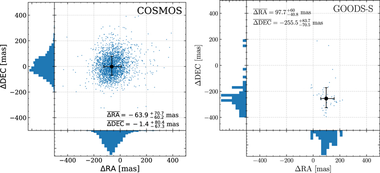
Figure 15. Scatter diagrams and histograms of offsets between the Gaia reference frame and the COSMOS2015 (left panel) and 3D-HST (ECDFS; right panel) catalogs. The offsets are in the sense “Gaia–COSMOS” and “Gaia–ECDFS,” respectively. For COSMOS, we find only a systematic offsets in R.A. direction of −64 mas. For ECDFS, the offsets are large in both directions. In addition to this, we measure a scatter in the astrometry of ∼100 mas for both fields in both coordinates.
Download figure:
Standard image High-resolution imageTo compute the astrometric offset of individual ALPINE galaxies, we make use of the fact that the HST images are already aligned to the Gaia reference frame (see details in Sections 3.1 and 3.2). Specifically, we compute the offsets between the coordinates measured on the ACS/F814W images and the original coordinates from the 3D-HST or COSMOS2015 catalog. If no ACS F814W image is available or if the galaxy is not detected (which happens for redshifts z > 5), we use the deepest image red of F814W. If none are available (in four cases), we report the average offset as shown in Figure 15.
Note that the coordinates given in the final ancillary data catalog are not corrected for these offsets. However, we give the offsets for each galaxy in the columns delta_RA and delta_DEC, which can be added to the original coordinates to obtain Gaia-corrected R.A. and declination (see Appendix A).
4. Physical Properties
In this section, we detail measurements of various basic physical properties of the ALPINE galaxies that are based on their total, extinction-corrected photometry described in Section 3. These include physical quantities from SED fitting such as stellar masses, SFRs, ages, and dust attenuation (Section 4.1), and UV continuum slopes (Section 4.3), as well as quantities directly derived from the photometry such as UV magnitudes and luminosities (Section 4.2) and estimates of the Hα luminosity and equivalent width from Spitzer colors (Section 4.4).
4.1. Stellar Mass and SFRs from SED Fitting
4.1.1. Fitting Method
For consistency and comparability with other studies on the COSMOS field, we choose the LePhare SED fitting code44 (Arnouts et al. 1999; Ilbert et al. 2006) to derive stellar masses, SFRs, light-weighted stellar population ages, absolute magnitudes, optical dust reddening, and UV continuum slopes of the ALPINE galaxies.
Importantly, stellar masses, SFR, and sSFR values are computed from the marginalized probability distribution functions over all of the models and uncertainties are given in ±1σ of this distribution.
We use a set of synthetic templates based on the Bruzual & Charlot (2003) stellar population library, which we tune to represent best galaxies at redshifts between 4 < z < 6. In detail, we use a series of different star formation histories (SFH) based on exponentially declining (with τ = 0.1, 0.3, 1.0, and 3.0 Gyr), delayed45
(with τ = 0.1, 0.5, 1.0, and 3.0 Gyr), and constant star formation. We add dust attenuation corresponding to a stellar  from 0 to 0.5 spaced in steps of 0.05 assuming a Calzetti et al. (2000) dust attenuation law. To account for metallicity dependence, we use a solar (
 ) and
) and  metallicity. We also adopt a Chabrier (2003) IMF in the following. The model SEDs are generated for logarithmically spaced ages starting from 50 Myr to the age of the universe at the redshift of each galaxy. To each SED, various rest-frame UV and optical emission lines are added following the description in Ilbert et al. (2009) by using common conversions outlined in Kennicutt (1998). Specifically, the UV luminosity at 2300 Å is converted to an SFR using the relation
  and subsequently translated to an [
 ] emission line flux using the relation
 ![$\mathrm{SFR}({{\rm{M}}}_{\odot }\,{\mathrm{yr}}^{-1})=(1.4\pm 0.4)\times {10}^{-41}\,{L}_{[\mathrm{OII}]}(\mathrm{erg}\,{{\rm{s}}}^{-1})$](https://content.cld.iop.org/journals/0067-0049/247/2/61/revision1/apjsab7ccdieqn205.gif) . Other emission lines (Lyα, [
. Other emission lines (Lyα, [ ], Hβ, Hα) are derived by assuming specific ratios to [
 ] that are calibrated by observations (see detailed description with references in Ilbert et al. 2009).
The models are fit to the photometry described in Section 3 (and listed in Tables 2 and 3). Specifically, for the galaxies in the ECDFS field, we use the ground-based observations in U, R, Jv, Hv, and  , as well as the intermediate-bands IA427, IA505, IA527, IA574, IA624, IA679, IA738, IA767, and IA856, and all four Spitzer channels ch1, ch2, ch3, and ch4. We also include observations in the HST filters F435W, F606W, F775W, F814W, F850LP, F125W, F140W, and F160W that are properly combined with the ground-based and Spitzer measurements in the 3D-HST catalog. For galaxies in the COSMOS field, we include the ground-based observations in u*, B, V, r+, i+, z++, Y, YHSC, J, H, Hw, Ks, and
  , as well as the intermediate-bands IA427, IA464, IA484, IA505, IA527, IA574, IA624, IA679, IA709, IA738, IA767, and IA827. We use all four Spitzer channels but no HST observations as only the one filter (F814W) exists for all galaxies.
The fits are performed in flux density space (fν in Jansky), which has several advantages compared to magnitude space. Specifically, it allows a proper statistical treatment of limits in the data of all bands. While in the case of magnitude limits, an arbitrary significance level (e.g., 1σ, 3σ) has to be defined in order to use them in SED fitting, in flux density space no arbitrary choice needs to be made by the user as the limits manifest themselves only in the error bars of those bands where no flux is measured. This is important, as slightly different levels of significance set for the limits can have profound effects on the output parameters, especially in cases where limits are imposed in astrophysically important parts of the rest-frame spectra (e.g., the Balmer break). In addition, some SED codes, including Le Phare, have difficulties dealing with limits (in the case of magnitudes) in a statistically consistent manner, and, instead, remove from consideration any models that slightly exceed these limits. Moving to flux density space for all fits alleviates these concerns.
Several studies have found that the photometric errors are generally underestimated (e.g., Ilbert et al. 2006, 2009, 2013; Skelton et al. 2014; Laigle et al. 2016). Artificially increasing the errors has been found to mitigate issues associated with poorly measured bands, poorly estimated zero-points, or inhomogeneous methods of measuring photometry. To avoid artificially small errors that would dominate the χ2 budget of a fit of a given galaxy, we follow the prescription of Laigle et al. (2016) and rescale the official flux density errors by a factor of 1.1. In addition, following Ilbert et al. (2009), we correct for underestimated photometric errors due to varying PSF sizes between optical and Spitzer imaging by adding in quadrature the following systematic errors to the photometric error budget prior to fitting: 0.01 mag for all ground-based UV/optical broadband measurements; 0.05 mag for all ground-based UV/optical intermediate-bands and near-IR broadband measurements; 0.1 mag for Spitzer  and
and  and 0.3 mag for Spitzer 5.8 and
  measurements.
The large PSF sizes of the Spitzer observations result in a large risk of blended photometry. This can lead to an overestimation of flux and, hence, to an overestimation of stellar masses.46
A cleaner and manual deblending of the Spitzer photometry (e.g., using a position prior from HST imaging) is possible and will be pursued in a forthcoming paper. In the following, we flag galaxies that have a bright companion galaxy within a Spitzer  PSF FWHM (2
5) based on the ground-based and HST imaging data. In total, one-third of the galaxies have contaminated Spitzer photometry to some degree. For 19% of the galaxies, the Spitzer photometry is severely contaminated and should not be trusted. We checked our simple flagging scheme against the contamination flags given in the 3D-HST catalog, which are based on the flux fraction that is overlapping with the galaxy for which the photometry is measured. For the 13 ALPINE galaxies in ECDFS, we find excellent agreement between both classifications. The Spitzer contamination flags are included in the ancillary data catalog (column spitzer_cont).
4.1.2. Systematic Uncertainties in Physical Properties from Modeling Assumptions
Depending on their exact methods, different SED-fitting codes may measure different physical properties even with the same photometry provided as input. In addition to more physical reasons (such as different assumptions on the stellar population models and implementation of emission lines), the different treatment of undetected fluxes (or fitting in magnitude space), varying minimization techniques and weightings, and different scaling of the error of the input photometry can contribute to these discrepancies.
To investigate the amplitude of such differences, we compare the measurements from LePhare to a modified version of the HyperZ code (Bolzonella et al. 2000) that includes the effects of nebular emission (Schaerer & de Barros 2009), to estimate such systematic uncertainties in the fitted parameters. To minimize the degeneracy with other assumptions, we run HyperZ on the exact same photometry and with the exact same model SEDs (i.e., same metallicity, age, SFH, and dust attenuation law) as described in Section 4.1.1. Figure 16 compares the stellar mass (left panel), SED-derived SFR (middle panel), and absolute UV magnitude (right panel, see also Section 4.2) derived by the two codes. The symbols are color-coded by difference in stellar population age (positive values indicate younger ages derived by HyperZ). We find that the stellar masses derived by HyperZ are systematically smaller by 0.3–0.4 dex. Similarly, the SFRs are systematically larger by ∼0.3 dex.
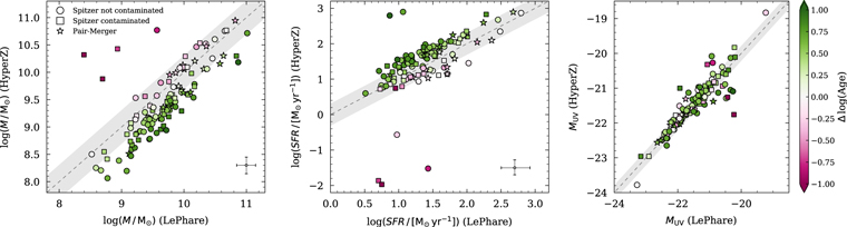
Figure 16. Comparison of stellar mass (left panel), SED-derived SFR (middle panel), and absolute rest-frame UV magnitude (right panel) measured by LePhare and HyperZ. The symbols are color-coded by the logarithmic difference in stellar population age (note that the scale is the same for all panels). The squares denote galaxies whose Spitzer photometry is blended with a nearby bright galaxy or star. The star-symbols denote mergers based on the classification in Le Fèvre et al. (2019). The 1–1 relation is shown as dashed line and a ±0.3 margin is shown by the gray band. The systematic differences in stellar masses derived by HyperZ are likely caused by different implementations of rest-frame optical emission lines, which affect most of the measurements of stellar masses (based on rest-frame optical light).
Download figure:
Standard image High-resolution imageAs expected, the absolute UV magnitudes are largely in agreement, as they are, to the first order, independent of the physical parameters and just represent a translation of the fitted UV flux.
The differences in stellar mass and SFR are due to the effect of nebular emission, which results in younger ages and larger emission line corrections of the intrinsic rest-frame optical continuum (observed by the Spitzer broad bands) in the HyperZ models, and therefore directly affects the stellar mass measurements (see, e.g., de Barros et al. 2014). This is confirmed by the fact that the stellar masses and SFR measured by the two codes agree well (within a factor of two) if the emission lines are turned off. The effect of nebular emission found by HyperZ may be overestimated for the ALPINE galaxies, e.g., if the emission lines are more strongly attenuated than the continuum (see Section 4.4). For consistency and comparability with other studies on the COSMOS field, we choose the LePhare fitting results as the default.
Next to the systematic offset discussed above, we also find four galaxies (DC_472215, DC_503575, DC_722679, DC_790930) whose stellar mass measurements are significantly discrepant, by more than one order of magnitude, between the two codes. Specifically, they are fitted with an old, low-SFR, and massive galaxy template with HyperZ, while a young, high-SFR, and low-mass galaxy template is preferred by LePhare. Three of these outliers have significantly contaminated Spitzer photometry (indicated by the squares). As a consequence, the apparent Spitzer fluxes and stellar masses are overestimated and the optical colors are artificially reddened, which makes their stellar masses largely unreliable. Furthermore, we artificially increased the errors of the Spitzer photometry in our LePhare measurements (see Section 4.1.1), hence they have smaller weights, which might reduce the effect of photometric contamination on the fit.
In addition, we investigate the effect of different dust reddening laws on the LePhare measurements. For this, we compare a Calzetti et al. reddening with a Small Magellanic Cloud (SMC; Prevot et al. 1984) reddening. The latter might be more suitable for metal-poor low-mass galaxies. Running LePhare with the same settings but adopting an SMC reddening curve, we find only small changes in the stellar mass and SFR measurements. Specifically, for the former, we find an average offset toward lower stellar masses in the case of SMC dust of 0.05 dex and a maximal offset of 0.2 dex. For latter, we find similar offsets toward lower SFRs in the case of SMC dust.
Finally, we note that the galaxy properties derived here are consistent within a factor of two with the ones published in the COSMOS2015 catalog (based on photometric redshifts). We conclude this from comparing galaxies with the same spectroscopic and photometric redshift within 0.1.
4.1.3. The ALPINE Galaxies on the z = 5 Main-sequence and [C ii] Fluxes
Figure 17 summarizes the results of this section by showing the relation between stellar mass and SFR (the main sequence) of our ALPINE galaxies together with the [ ] emission (in
  ) measured by ALMA (in color). The measurements are compared to all galaxies (with photometric redshifts) at 4 < z < 6 in the COSMOS2015 catalog (blue points) as well as the main-sequence parameterization by Speagle et al. (2014) at z = 5 (gray band with ±0.3 dex width).
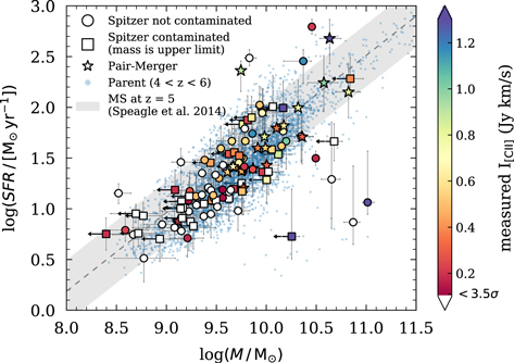
Figure 17. Relation between stellar mass and SFR (main sequence) of our ALPINE galaxies compared to all COSMOS galaxies at 4 < z < 6 (blue points) and the main-sequence parameterization at z = 5 by Speagle et al. (2014) (gray band with ±0.3 dex width). Galaxies with contaminated Spitzer photometry are marked with squares (their stellar mass is likely an upper limit) and mergers (classification by Le Fèvre et al. 2019) are shown as stars. The color denotes the [ ] flux in
  measured by ALPINE. Galaxies that are not detected at the 3.5σ level are shown with white face color.
Download figure:
Standard image High-resolution imageThe comparison to the photometrically selected COSMOS parent sample indicates that the ALPINE sample is a fair representation of the overall population of star-forming z > 4 galaxies. The sample also includes at higher stellar masses galaxies that lie 2–3σ below the main sequence. Note that two of these galaxies at  ∼ 10.3 and 10.7 have contaminated Spitzer photometry, and therefore, their stellar masses are upper limits. Other two galaxies at
  and 10.9 do not show [
 ] emission, which is expected if they are systems of low SFR below the main sequence. The galaxy with [
 ] detection at
  is classified as “extended dispersion dominated” by our [
 ] morpho-kinematic classification (see Le Fèvre et al. 2019) and the HST/ACS imaging suggest a clumpy morphology. Although significantly below the main sequence, [
 ] is still detected in that galaxy, perhaps indicative of dust-obscured star formation.
The color-coding of the points suggests a [ ] emission increase along the star-forming main sequence. Furthermore, the fraction of [
 ] detected galaxies significantly drops below
  or an SFR of less than
  . This could be due to the effect of metallicity on the [
 ] line strength by either indirectly a higher ionization state or directly through lower Carbon abundance (e.g., Narayanan et al. 2018). The relationship between star formation and [
 ] emission will be studied in more detail in a forthcoming paper (Schaerer et al. 2020).
Note that there are galaxies with an SFR of less than  in our sample, contrary to our initial selection. We emphasize that the initial selection was based on the observed absolute UV magnitude and not on any property derived from SED fitting (such as SFR). This discrepancy is therefore expected within the uncertainty of measuring SFRs from SED fitting.
4.2. Measurement of UV Magnitudes and Luminosities
The UV luminosities and absolute UV magnitudes at rest frame 1500 Å (not dust corrected) are measured during the SED-fitting process with LePhare and are defined by the transmission curve of the Galaxy Evolution Explorer (GALEX) FUV filter (∼1500 Å). As shown in Section 4.1.2, the absolute UV magnitudes measured by LePhare and HyperZ are in very good agreement.
We also compare these measurements to a more direct method by using the observed flux in a single filter that is closest to rest frame 1500 Å (Subaru z++ filter at z < 5 and UltraVISTA Y or YHSC band at z > 5 for galaxies in COSMOS and the HST filter F850LP for all of the galaxies in ECDFS). The left panel in Figure 18 shows a very good agreement between the two methods. The scatter is mainly due to the low S/N of the single-filter measurements of the second method (indicated by the large error bars). The scatter is enhanced for galaxies at z > 5 also due to the fact that the UltraVISTA Y-band observations are less deep than the z++ observations used for z < 5 galaxies. In the following, we will use the more robust absolute UV magnitude from LePhare as they depend less on the S/N of single observations.
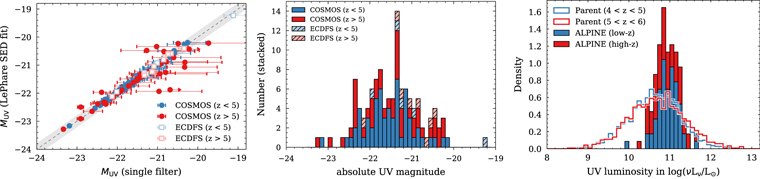
Figure 18. Left panel: comparison of absolute UV magnitudes derived from LePhare and from one single filter close to rest frame 1500 Å. The scatter at fainter magnitudes is an S/N effect in the latter measurement. The gray stripe shows ±0.3 magnitudes around the one-to-one line. Middle panel: distribution of absolute UV magnitudes of the whole ALPINE sample. Right panel: the UV luminosity distribution of ALPINE galaxies in relation to a parent sample from the COSMOS2015 catalog selected in the same redshift range. ALPINE galaxies occupy brighter luminosity, caused by the selection in MUV (see Section 2.1).
Download figure:
Standard image High-resolution imageThe middle panel in Figure 18 shows the distribution of absolute UV magnitudes for galaxies in the COSMOS and ECDFS fields in two redshift bins as in the previous figures. The bulk of galaxies are between MUV of −22.7 and −20.2 (consistent with the faint absolute UV magnitude limit of the survey, see Section 1.2). One of the galaxies in ECDFS (CANDELS_GOODSS_37) is significantly fainter (MUV = −19.2). This galaxy has been added to the sample to fill in an empty frequency window. The measurement of the absolute UV magnitude from single band and SED fit agree and the galaxy is compact and isolated (i.e., no contamination in the photometry). The fit to its photometry with LePhare suggests a dust-free, low-mass ( = 9.22) galaxy that is forming stars at a rate typical for the main sequence (
![$\mathrm{log}(\mathrm{SFR}/[{{\rm{M}}}_{\odot }\,{\mathrm{yr}}^{-1}])=0.97$](https://content.cld.iop.org/journals/0067-0049/247/2/61/revision1/apjsab7ccdieqn233.gif) ).
).
The right panel of Figure 18 compares the distribution of the UV luminosity of the ALPINE galaxies (stacked filled histogram for low and high redshift) to the same parent sample selected from the COSMOS2015 catalog and used in Figure 17 split in two redshift bins (empty histogram). As expected, the absolute UV magnitude cut applied for the selection of the ALPINE sample (see Section 2.1) causes a bias toward the brighter end of the parent distribution.
4.3. UV Continuum Slopes
4.3.1. Method
The UV continuum slope (β, defined as  ) generally correlates with the attenuation of stellar light by dust and is therefore an important tool to study the dust properties of galaxies especially at high redshfits (e.g., Meurer et al. 1999; Bouwens et al. 2009; Finkelstein et al. 2012). The UV continuum slope of a galaxy can be derived by various methods. Here, we compute β from the best-fit SEDs derived by LePhare. Compared to deriving the slopes directly from the observed photometry by a linear fit, this approach results in less-biased β measurements in the case of low-S/N observations (e.g., Finkelstein et al. 2012; Barisic et al. 2017). This is particularly true for the ALPINE galaxies, whose rest-frame UV continuum is predominantly covered by relatively shallow ground-based imaging. Deep HST coverage by a sufficient number of bands of this wavelength range is only available for a small fraction of the galaxies.
The β slopes are derived by a robust linear fit (to avoid the fit being affected by any absorption or emission lines) to the logarithmic slope of the best-fit LePhare SED in the wavelength range between  and 2300 Å. To quantify uncertainties, we perturb the fluxes of each filter according to their individual errors assuming a Gaussian error distribution, refit the galaxies, and re-measure β from the resultant best-fit SED. For each galaxy, we repeat this procedure 1000 times to produce a probability density function. The uncertainties for β quoted here are the 1σ percentiles of this distribution and are, on average, on the order of Δβ = 0.2–0.3.
4.3.2. Systematic Uncertainties and Dependencies on Dust Attenuation
In addition to photometric uncertainties, several model assumptions affect the measurement of β. We found that the two most important ones are the wavelength range over which β is fit and the assumed dust attenuation law.
We choose the wavelength range over which β is measured to be consistent with the definition of several other studies (Calzetti et al. 1994; Meurer et al. 1999; Finkelstein et al. 2012; Bouwens et al. 2014; Barisic et al. 2017; Fudamoto et al. 2017). In the upper panel of Figure 19, we demonstrate how the β measured for our ALPINE galaxies would change if different wavelength ranges are used. First, we do not find any differences in our measurements compared to the definition by Calzetti et al. (1994), who use 10 discrete fitting windows between 1300 Å and 2600 Å to avoid strong absorption and emission lines (green diamonds). The other symbols show the comparison to different wavelength ranges, and we notice significant offsets from our measurements. For example, defining β between 1600 Å and 2200 Å results in up to Δβ = 0.1 bluer slopes (orange squares). Using a significantly redder wavelength range, 1600 Å to 2600 Å, leads to 0.1–0.35 bluer slopes (blue circles) compared to our definition. Note that the offset varies as a function of β itself—specifically, differences are enhanced toward redder slopes.
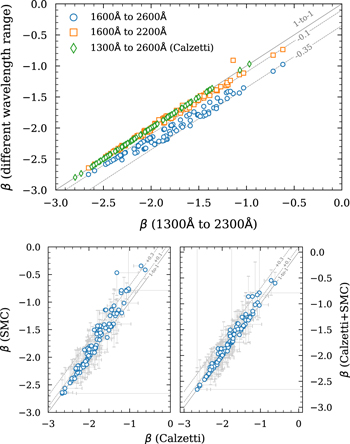
Figure 19. Dependence of UV continuum slope β on the definition of the wavelength regions and assumption of dust attenuation law. The solid line shows the 1–1 relation and the dashed lines show different offsets. Top panel: dependence of β on the adopted wavelength window (with respect to our choice, 1300 Å–2300 Å). Bottom panel: dependence of β on the assumed dust attenuation law. Using an SMC dust attenuation results in redder slopes compared to a Calzetti reddening law.
Download figure:
Standard image High-resolution imageThe second, more physically driven quantity that affects the measurement of β is the assumed dust attenuation law. As described in Section 4.1.2, the choice of the dust attenuation law has a negligible affect on the stellar masses and SFRs. This is not the case for the β slopes as shown in the lower panels of Figure 19. The left panel compares β derived using Calzetti and SMC dust attenuation. We notice a consistent positive offset of up to Δβ = 0.3 for the reddest slopes. We compared the reduced χ2 values output by LePhare for fits using a Calzetti and SMC dust attenuation in order to derive a preference for either of the dust attenuations. We find that the χ2 values show insignificant differences, which lets us conclude that we are not able to distinguish between the different dust attenuations based on our SED fitting. Hence, we decided that the best way is to be agnostic about the dust attenuation and combine for each galaxy the two probability density functions PCalzetti(β) and PSMC(β) derived from our Monte Carlo approach (Section 4.3.1) assuming equal weighting to derive the median β and its 1σ uncertainties. In the lower left panel of Figure 19, the final combined β slopes are compared to the β derived assuming a Calzetti attenuation. The offset toward redder β is significantly reduced due to narrower probability density functions, assuming Calzetti dust (hence, the average β is drawn to the Calzetti solution in most cases).
4.3.3. The β Slopes of the ALPINE Galaxies in Context
Figure 20 shows our β measurement (marginalized over both Calzetti and SMC dust) as a function of stellar mass split in the different methods of selection (Section 2.1). As the UV slope is mostly affected by the dust attenuation, the strong correlation between β and stellar mass is not surprising as more massive galaxies are expected to be more dusty. The z ∼ 5.5 narrowband-selected galaxies, statistically, have the bluest slopes, indicating their dust-poor nature. The other galaxies are spread out over the whole parameter space. We also show the data from our parent sample at 4 < z < 6 in gray and compare their β slope and stellar mass distribution to the ALPINE sample in the kernel density estimate plots. Note that the β slope distribution of ALPINE galaxies peaks at Δβ ∼ 0.2 bluer values than the parent sample at the same redshift. This is a minor bias (likely caused by our spectroscopic selection) that has to be kept in mind for future analyses.
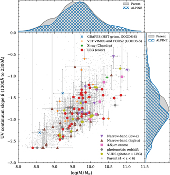
Figure 20. Comparison of UV slopes and stellar mass. The offset panels show kernel density estimates of the β and stellar mass distribution. The ALPINE galaxies (large symbols) are split into their method of selection (see Section 2.1). We also show the data from our parent sample at 4 < z < 5 (gray dots). Statistically, our ALPINE peaks at ∼0.2 dex higher stellar masses and ∼0.3 bluer β.
Download figure:
Standard image High-resolution image4.4. Measurement of Hα Emission
Rest-frame optical emission lines in z > 4 galaxies are out of reach of current spectrographs. Specifically, the Hα emission provides a good tool to study the star formation properties of galaxies in more detail. Fortunately, in the redshift range 4 < z < 5, the Hα line falls in the Spitzer  filter, while the
  filter lacks any strong emission lines. Therefore, the [
 ]−[
]−[ ] color can be used to constrain the Hα line flux and its equivalent width (a proxy of recent stellar mass build up). This method leads to Hα emission properties that are statistically as accurate as derived from spectroscopic data (Faisst et al. 2016a). Several such measurements have been carried out in the past with success (Shim et al. 2011; Stark et al. 2013; de Barros et al. 2014; Smit et al. 2014; Mármol-Queraltó et al. 2016; Faisst et al. 2016a; Rasappu et al. 2016; Smit et al. 2016; Caputi et al. 2017; Faisst et al. 2019).
About 55% of the ALPINE sample (66 galaxies) lie in this redshift range. To measure the Hα luminosity and equivalent widths, we follow the same technique as outlined in Faisst et al. (2019; we refer to this paper for more technical details). In brief, this method makes an assumption on the rest-frame optical continuum to which emission lines are added in a consistent manner to reproduce the observed [ ]−[
]−[ ] colors of the galaxies. This approach is robust, as it only depends on the slope of the rest-frame optical continuum, which is well defined and nearly independent of assumptions on age, metallicity, and star formation history for galaxies younger than ∼1 Gyr (mostly the case at z > 4). To describe the rest-frame optical continuum, we use several basis stellar population models based on the Bruzual & Charlot (2003) template library (see Table 4). For the dust correction of the Hα emission, we assume the stellar
  values derived by LePhare, which we convert to nebular extinction factors by assuming an f-factor47
of 0.44 as measured in local starburst galaxies (Calzetti et al. 2000). We also assume a Calzetti and SMC reddening law. Furthermore, we assume an [
values derived by LePhare, which we convert to nebular extinction factors by assuming an f-factor47
of 0.44 as measured in local starburst galaxies (Calzetti et al. 2000). We also assume a Calzetti and SMC reddening law. Furthermore, we assume an [ ] to Hα ratio of 0.15, as expected for galaxies at
  (Faisst et al. 2018), to correct the blending of the [
 ] and Hα lines.
Table 4. List of Basis Stellar Population Models for the Parameterization of the Rest-frame Optical Continuum at 4 < z < 5 to Derive Hα Emission from Spitzer Colors
| Model | SFH | Metallicity | Dust attenuation |
|---|---|---|---|
| (Z⊙ = 0.02) | |||
| A | Constant | 0.02 | Calzetti |
| B | Constant | 0.004 | Calzetti |
| C | Exp. declininga | 0.01 | Calzetti |
| D | Constant | 0.02 | SMC |
| E | Constant | 0.004 | SMC |
| F | Exp. declininga | 0.01 | SMC |
Note.
aAssuming .
.
Download table as: ASCIITypeset image
In Figure 21, we show systematic uncertainties in the measurement of the Hα luminosity due to the assumptions in our model for the rest-frame optical continuum and the reddening law (models A through F, see Table 4), as well as the f-factor for  and 0.4. It is evident that different assumptions in metallicity and SFH have a negligible impact on the measured Hα luminosity. The choice of the reddening law matters as the Hα luminosity decreases by ∼0.3 dex for galaxies at high Hα luminosities (
 ) assuming an SMC reddening law. The f-factor is the largest uncertainty in this measurement method and will have to be pinned down by future observations with the JWST. For now, the assumed f = 0.44 provides likely an upper limit on the Hα luminosities. As shown by the arrows in Figure 21, assuming an f-factor equal to unity (which is thought to be more likely based on observations at z ∼ 2) would decrease the Hα luminosities by up to 0.4 dex (0.8 dex) for a stellar dust reddening of 0.2 (0.4) magnitudes. The correction in the case of an SMC reddening law are 0.1–0.2 dex less. We note that these factors also apply to Hα-derived SFRs and any other quantity that depends linearly on the Hα luminosity.
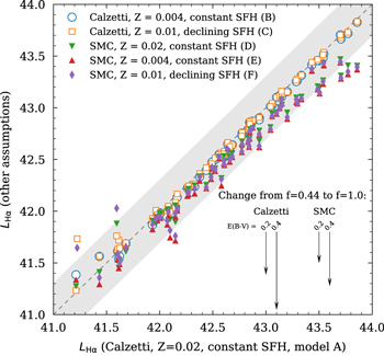
Figure 21. Effect of different assumptions of the rest-frame optical continuum, reddening law, and f-factor (arrows show absolute decrease in luminosity from f = 0.44–1.0 for different stellar dust attenuations and reddening laws) on the measurement of the Hα luminosity. The gray band shows the 1–1 relation with ±0.3 dex margin. The different models for the continuum are labeled in the same way as in Table 4). The f-factor (differential reddening between stellar continuum and nebular regions) has the strongest effect on the Hα luminosity measurements.
Download figure:
Standard image High-resolution imageThe top panel of Figure 22 compares the SFRs derived from SED fitting (Section 4.1) to the Hα luminosity and Hα-derived SFRs for galaxies without contaminated Spitzer photometry. The latter is derived using the standard conversion factor given in Kennicutt (1998),

assuming solar metallicity and a Chabrier IMF. Assuming one-fifth solar metallicity, the inferred SFR is expected to be ∼0.2 dex lower (Ly et al. 2016). As shown in Faisst et al. (2019), the uncertainty of this conversion factor is negligible compared to the impact of the uncertain f-factor. The Hα luminosities in the ALPINE sample range from  to
to  assuming f = 0.44 and Calzetti et al. (2000) dust attenuation. The Hα-derived SFRs trace well the SED-derived SFRs above
  . Below that value, we see a large scatter in Hα derived SFRs, which happens when the Hα emission becomes too faint to be measured reliably using the Spitzer broad bands. Specifically, this is the case roughly at
  , which corresponds to a 4.5 μm detection of less than 5σ (see Figure 3 and the Appendix in Faisst et al. 2019).
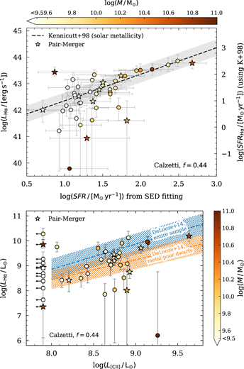
Figure 22. Top panel: comparison of SED-derived SFRs to Hα luminosity (left y-axis) and Hα-derived SFR (right y-axis). The latter are derived from Hα assuming the conversion factor by Kennicutt (1998) for solar metallicity (dashed line and ±0.3 dex margin, gray). Only galaxies with uncontaminated Spitzer photometry are shown. The symbols are color-coded by stellar mass. The star-symbols denote mergers based on the classification in Le Fèvre et al. (2019). The Hα-dependent quantities are derived assuming a Calzetti reddening law, constant SFH, solar metallicity, and f = 0.44 (see Figure 21 for effect of different assumptions). Above an SFR of  , the two SFRs are comparable. Below that threshold, the scatter in the Hα-derived SFRs increases due to low S/N of the
  observations (see Faisst et al. 2019). Bottom panel: comparison of Hα and [
 ] luminosity. Shown are only galaxies with Hα measurements and uncontaminated Spitzer photometry. [
 ] undetected galaxies (at <3.5σ) are indicated with upper limits. The lines and dashed margins show the expected relation between Hα and [
 ] derived combining the relations from Kennicutt (1998) and De Looze et al. (2014; for their entire sample and metal-poor dwarf galaxies, see the text). Note that at lower [
 ] luminosities (
 ), the galaxies seem to be more consistent with the relation of local metal-poor dwarf galaxies.
Download figure:
Standard image High-resolution imageThe lower panel of Figure 22 relates the Hα luminosity (here in units of solar luminosity) to the [ ] luminosity measured by ALMA (also solar luminosity). In addition, we show the expected relation between Hα and [
 ] luminosity by combining Equation (5) with the linear relation between [
 ] and SFR derived by De Looze et al. (2014) from local and low-redshift galaxy samples,

for different values of intercepts (γ) and slopes (α). Specifically, we are showing the relation for their entire sample (α = 1.01, γ = − 6.99, blue hatched) and the metal-poor dwarf galaxies (α = 0.80, γ = − 5.73, red hatched). For bright [ ] galaxies (
![${L}_{[{\rm{C}}{\rm{I}}{\rm{I}}]}\gtrsim 5\times {10}^{8}\,{L}_{\odot }$](https://content.cld.iop.org/journals/0067-0049/247/2/61/revision1/apjsab7ccdieqn265.gif) ), we find a good agreement with the entire local sample. For lower [
), we find a good agreement with the entire local sample. For lower [ ] luminosities, the Hα measurements fall below this relation and are instead more consistent, although with a large scatter, with the relation of metal-poor local dwarf galaxies. The majority of [
 ] undetected galaxies align well with either relation, however, the uncertainty in the Hα measurements becomes substantial as galaxies fall below
  .
.
Figure 23 shows the rest-frame Hα EW distribution of our ALPINE galaxies in the context of local galaxies (gray cloud) and other z ∼ 4.5 galaxies on the COSMOS field (gray, Faisst et al. 2019). The Hα EW for the z > 4 galaxies is derived consistently assuming a constant SFH, Calzetti reddening law, and f = 0.44. The ALPINE galaxies cover the parameter space of the other z ∼ 4.5 galaxies and, hence, build a representative sample also in terms of Hα properties. For a fixed stellar mass, the high-redshift galaxies have higher Hα EWs compared to local galaxies, which is expected from a galaxy evolution point of view as galaxies at higher redshift are highly star-forming. Note that two galaxies in the ALPINE sample have similar Hα EW values as massive ( ) local galaxies. Consistently, also their sSFR are low (
 ), which is indicative of them being systems with evolved stellar populations at high redshifts.
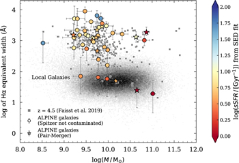
Figure 23. The rest-frame Hα EW of our ALPINE galaxies in context of local galaxies (gray cloud) and z = 4.5 galaxies from Faisst et al. (2019) (gray squares). The Hα EW is related to stellar mass and sSFR derived from SED fitting (color-coded). The ALPINE sample at 4 < z < 5 builds a representative subsample of the general galaxy population at z > 4, also in terms of Hα properties. Although with similar stellar masses as local galaxies, the high-redshift galaxies reside at significantly higher Hα EWs, which is naturally explained by their higher star formation. Note the two galaxies with particularly low sSFR ( , and consistently low Hα EWs of less than
  ) that fall onto the massive end of the distribution of local galaxies. These galaxies are indicative for systems with evolved stellar populations at high redshifts with currently reduced star formation activity.
Download figure:
Standard image High-resolution image5. Summary and Conclusions
The early growth phase at redshifts z = 4–6 marks an important time in which galaxies build up their stellar mass, enrich in metals and dust, and change their structure to transform into galaxies at the peak of SFR density or thereafter. For a better understanding of this interesting galaxy population, a multiwavelength survey is crucial. ALPINE comprises a valuable set of 118 galaxies at 4.4 < z < 5.9 with unprecedented ALMA data at ∼150 μm FIR wavelengths. Together with the ancillary data presented in this paper, it makes it the first large panchromatic survey to discover the formation and study the evolution of galaxies during the early growth phase.
Summarizing, the science enabling corner stone data sets of ALPINE are:
- 1.Unprecedented ALMA observations to study the dust, gas, and outflow properties of the largest sample of galaxies to-date at z > 4 (Bethermin et al. 2020),
- 2.
- 3.Coherent ground-based (and space-based in ECDFS) imaging data from the optical to near-IR (Section 3) for the measurement of various properties from SED-fitting methods (Section 4.1), including stellar masses and SFRs (Section 4.1.1), UV luminosities (Section 4.2), and UV continuum slopes to study stellar dust attenuation (Section 4.3),
- 4.
- 5.High-resolution HST/ACS imaging in F814W for all galaxies and WFC3/IR imaging for a smaller fraction (less than 30% with deep F160W data) to study their resolved structure in connection with FIR [] emission (Section 3).


The ALPINE sample is built upon several different selection methods (Section 2.1, Figure 3) and, hence, contains a multitude of different spectroscopic properties. Because of the requirement for spectroscopic confirmation, the sample is slightly biased toward brighter UV magnitudes (Section 4.2, Figure 18) and blue UV continuum slopes (Δβ ∼ 0.2) compared to the average 4 < z < 6 galaxy population (Section 4.3, Figure 20). Nonetheless, stellar masses and SFRs, derived from the wealth of ancillary data, show that the ALPINE sample is broadly representative of the 4 < z < 6 galaxy population.
The FIR [ ] redshifts observed by ALMA allow us to set the systemic redshift of the galaxies in order to study velocity offsets of Lyα emission and several rest-frame UV absorption lines (Section 2.4). From one galaxy at z = 4.57 with optical [
 ] measurements acquired from Keck/MOSFIRE, we show that the [
 ] and FIR [
 ] redshifts are in excellent agreement; hence, the latter likely is a good tracer of the systemic redshift derived by optical emission lines at lower redshifts (Section 2.4.3, Figure 11). In general concordance with studies at z = 2–3 (using Hα to define the systemic redshift), we find that on average that Lyα is redshifted (∼180 km s−1) with respect to the [
 ] line, while the absorption lines are blueshifted (
 ). In Cassata et al. (2020), we perform a more detailed comparison to samples at lower redshifts and study the implication on the Lyα escape fraction in correlation with Lyα equivalent widths. Stacking the spectra in bins of sSFR, we find larger velocity offsets of absorption lines with respect to systemic for galaxies with high sSFRs, which is indicative of stronger winds and outflows in these galaxies (Section 2.4.2, Figure 10). This finding is in agreement with the recent work by Ginolfi et al. (2020), who show a broadening in the FIR [
 ] profiles in ALPINE galaxies with high star formation.
Statistically, the SFRs derived from Hα emission via the Kennicutt (1998) relation for galaxies between 4 < z < 5 agree well with the values derived from SED fitting, assuming a differential dust reddening factor of f = 0.44 (Section 4.4, upper panel of Figure 22). However, we observe a considerable scatter for fainter galaxies ( ) due to the lower S/N of the Spitzer observations. Thanks to the large sample size of ALPINE, we are able, for the first time, to compare the Hα luminosity to the [
 ] luminosity (lower panel of Figure 22). Overall, we find Hα luminosities as expected from the local relation between
 ![${L}_{[{\rm{C}}{\rm{I}}{\rm{I}}]}$](https://content.cld.iop.org/journals/0067-0049/247/2/61/revision1/apjsab7ccdieqn286.gif) and SFR from De Looze et al. (2014) (using their fit to the entire sample). However, we find that at low [
and SFR from De Looze et al. (2014) (using their fit to the entire sample). However, we find that at low [ ] luminosities (
 ), the Hα luminosities are generally lower than what is predicted by that relation. Instead, the De looze et al. relation derived from a sample of metal-poor dwarf galaxies is a better fit for those galaxies. This might suggest a more complex relation between SFR and [
 ] luminosity driven by metallicity or other properties of the ISM.
ALPINE is the beginning of a thorough exploration of galaxies at z > 4. It builds the foundation onto which future follow-up observations can build on. In fact, several follow-up programs are being granted, some of which are already on going. These include (i) additional HST WFC3/IR observations of interacting ALPINE galaxies (PI: Faisst), (ii) follow-up observations of [ ] at
] at  with ALMA for nine ALPINE galaxies (PI: Faisst), (iii) high spatial resolution (
 ) observations of the brightest ALPINE galaxies (PI: Ibar), and (iv) the follow up of four serendipitous objects at z > 4 with NOEMA (PI: Loiacono & Béthermin). In addition, several JWST proposals are in preparation.
All ancillary data products (including catalogs, images, and spectra) will be made public accessible. In Appendix A, we detail the layout of the catalogs including the measurements detailed in this paper. In Appendix B, we show HST cutouts in ACS F814W and WFC3/IR F160W bands as well as the rest-frame UV spectra of all individual ALPINE galaxies.
This paper completes a series of three papers presenting the ALPINE survey (Le Fèvre et al. 2019) and the data processing (Bethermin et al. 2020).
We would like to thank numerous people for the exchange of data without which the ALPINE ancillary data paper would not exist. In particular, we would like to thank E. Vanzella for helping us gathering the spectra in the ECDFS field and O. Ilbert for useful discussions that improved the SED-fitting results. We also thank the anonymous referee for the suggestions that improved this paper. This paper is based on data obtained with the ALMA Observatory, under Large Program 2017.1.00428.L. ALMA is a partnership of ESO (representing its member states), NSF (USA) and NINS (Japan), together with NRC (Canada), MOST and ASIAA (Taiwan), and KASI (Republic of Korea), in cooperation with the Republic of Chile. The Joint ALMA Observatory is operated by ESO, AUI/NRAO and NAOJ. This program receives funding from the CNRS national program Cosmology and Galaxies. This work is based on observations and archival data made with the Spitzer Space Telescope, which is operated by the Jet Propulsion Laboratory, California Institute of Technology, under a contract with NASA along with archival data from the NASA/ESA Hubble Space Telescope. This research made also use of the NASA/IPAC Infrared Science Archive (IRSA), which is operated by the Jet Propulsion Laboratory, California Institute of Technology, under contract with the National Aeronautics and Space Administration. In parts based on data products from observations made with ESO Telescopes at the La Silla Paranal Observatory under ESO programme ID 179.A-2005 and on data products produced by TERAPIX and the Cambridge Astronomy Survey Unit on behalf of the UltraVISTA consortium. Based on data obtained with the European Southern Observatory Very Large Telescope, Paranal, Chile, under Large Program 185.A-0791, and made available by the VUDS team at the CESAM data center, Laboratoire d’Astrophysique de Marseille, France. This work is based on observations taken by the 3D-HST Treasury Program (GO 12177 and 12328) with the NASA/ESA HST, which is operated by the Association of Universities for Research in Astronomy, Inc., under NASA contract NAS5-26555. Furthermore, this work is based on data from the W. M. Keck Observatory and the Canada–France–Hawaii Telescope, as well as collected at the Subaru Telescope and retrieved from the HSC data archive system, which is operated by the Subaru Telescope and Astronomy Data Center at the National Astronomical Observatory of Japan. The authors wish to recognize and acknowledge the very significant cultural role and reverence that the summit of Maunakea has always had within the indigenous Hawaiian community. We are most fortunate to have the opportunity to conduct observations from this mountain. Finally, we would also like to recognize the contributions from all of the members of the COSMOS Team who helped in obtaining and reducing the large amount of multiwavelength data that are now publicly available through IRSA at http://irsa.ipac.caltech.edu/Missions/cosmos.html. A.C., F.P., M.T., C.G., and F.L. acknowledge the support from grant PRIN MIUR 2017. G.C.J. acknowledges ERC Advanced Grant 695671 “QUENCH” and support by the Science and Technology Facilities Council (STFC). E.I. acknowledges partial support from FONDECYT through grant No. 1171710. The Cosmic Dawn Center (DAWN) is funded by the Danish National Research Foundation under grant No. 140. S.T. acknowledges support from the ERC Consolidator Grant funding scheme (project Context, grant No. 648179). L.V. acknowledges funding from the European Union’s Horizon 2020 research and innovation program under the Marie Sklodowska-Curie grant agreement No. 746119. D.R. acknowledges support from the National Science Foundation under grant Nos. AST-1614213 and AST-1910107 and from the Alexander von Humboldt Foundation through a Humboldt Research Fellowship for Experienced Researchers.
Appendix A: Description of Published Data Products
The data presented in this paper are summarized in three different catalogs.
- 1.The main catalog, which contains properties consistently measured for all of the galaxies. These include general information (such as coordinates, redshifts, selection, morphological class), measurements performed on the spectra (such as Lyα redshift and properties as well as absorption line redshifts), measurements from SED fitting (including UV continuum slopes), and Hα line properties and SFRs.
- 2.The ECDFS photometry catalog, which contains all of the Galactic extinction-corrected total photometry (magnitude, fluxes, and uncertainties) of the galaxies in the ECDFS field. This catalog is based on the 3D-HST catalog.
- 3.The COSMOS photometry catalog, which contains all of the Galactic extinction-corrected total photometry (magnitude, fluxes, and uncertainties) of the galaxies in the COSMOS field. This catalog is based on the COSMOS2015 catalog.
The following Tables A1, A2, and A3 summarize the columns of each of these three catalogs. The catalogs can be downloaded in FITS format at http://alpine.ipac.caltech.edu.
Table A1. Column Description of Main Catalog
| Column | Unit | Description |
|---|---|---|
| General information and selection | ||
| ALPINE_ID | ⋯ | Unique name for each galaxy in string format |
| RA | degrees | R.A. in J2000 in degrees from either the COSMOS or 3D-HST catalog |
| delta_RA | milli-arcsec | Constant shift (to be added to RA) in R.A. due to astrometric offset (see Section 3.3) |
| DEC | degrees | decl. in J2000 in degrees from either the COSMOS or 3D-HST catalog |
| delta_DEC | milli-arcsec | Constant shift (to be added to DEC) in decl. due to astrometric offset (see Section 3.3) |
| field | ⋯ | Field name (1 = ECDFS or 2 = COSMOS) |
| selection | ⋯ | Original selection. For galaxies in the ECDFS field, this can be vlt or grapes. For galaxies in COSMOS, possible selections are CHANDRA, LBG, NB1a, NB2a, excess, photz, or vuds. See Section 2.1 and Table 1 for details. |
| z_orig | ⋯ | Original redshift used for initial selection (this redshift is derived from Lyα or absorption lines). |
| z_cii | ⋯ | Redshift determined from FIR [ ] emission lines (see details in Bethermin et al. 2020). Is −99 if [ ] emission lines (see details in Bethermin et al. 2020). Is −99 if [ ] is not detected at S/N > 3.5. ] is not detected at S/N > 3.5. |
| morph_class | ⋯ | Morpho-kinematic classes from Le Fèvre et al. (2019). Only for galaxies with >3.5σ [ ] detection(else class set to −99). The classes are: (1) rotator; (2) pair-merger (major or minor); (3) extended dispersion-dominated; (4) compact dispersion-dominated; (5) too weak for assigning a class. ] detection(else class set to −99). The classes are: (1) rotator; (2) pair-merger (major or minor); (3) extended dispersion-dominated; (4) compact dispersion-dominated; (5) too weak for assigning a class. |
| Measurements on spectra (Section 2) | ||
| has_twin | ⋯ | A flag set to 1 of for a galaxy has been observed by Keck/DEIMOS and VUDS (two spectra available). If false, the flag is set to 0. |
| z_lya | ⋯ | Redshift determined from peak of Lyα emission (see details in Cassata et al. 2020). Is −99 if no redshift measured. |
| lya_ew | Å | Observer-frame Lyα emission equivalent (see details in Cassata et al. 2020). Is −99 if no equivalent width is measured. |
| lya_ew_err | Å | 1σ uncertainty on observer-frame Lyα emission equivalent (see details in Cassata et al. 2020). Is −99 if no equivalent width is measured and −1 if no continuum measured (i.e., EW is upper limit). |
| f_lya | erg s−1 cm−2 | Lyα emission flux (see details in Cassata et al. 2020). Is −99 if flux is measured. |
| flag_specpro | ⋯ | Visual flag for reliability of absorption redshift measurements. Set to −99 if not attempted, then 1, 2, and 3 for least, medium, and most robust. |
| z_iswind | ⋯ | Redshift determined from IS+wind absorption lines (see Section 2.4). Set to −99 if no redshift measured. |
| z_iswind_low | ⋯ | Lower 95% percentile of redshift determined from IS+wind absorption lines. Set to −99 if no redshift measured. |
| z_iswind_up | ⋯ | Upper 95% percentile of redshift determined from IS+wind absorption lines. Set to −99 if no redshift measured. |
| n_lines_iswind_used | ⋯ | Number of lines used for IS+wind redshift measurement. We advise to generally only use galaxies with a value >2 together with flag_specpro >0 for a conservative sample selection. |
| z_wind | ⋯ | Redshift determined from wind absorption lines (see Section 2.4). Set to −99 if no redshift measured. |
| z_wind_low | ⋯ | Lower 95% percentile of redshift determined from wind absorption lines. Set to −99 if no redshift measured. |
| z_wind_up | ⋯ | Upper 95% percentile of redshift determined from wind absorption lines. Set to −99 if no redshift measured. |
| n_lines_wind_used | ⋯ | Number of lines used for wind redshift measurement. We advice to generally only use galaxies with a value >0 together with flag_specpro >0 for a conservative sample selection. |
| Properties from SED fitting with LePhare (Sections 4.1 and 4.2) | ||
| ID_photcat | ⋯ | ID in the photometric catalogs. This is the 3D-HST catalog for galaxies in ECDFS and the COSMOS2015 catalog for galaxies in COSMOS. |
| chi2 | ⋯ | χ2 value given by the LePhare fit. |
| Nband | ⋯ | Number of bands used for SED fitting. |
| ebmv | mag | E(B − V) derived from SED fitting. |
| logAge | yr | Logarithmic age |
| logAge_loweff1sig | yr | Lower 1σ limit on age in log |
| logAge_higheff1sig | yr | Upper 1σ limit on age in log |
| logMstar | M⊙ | Logarithmic stellar mass |
| logMstar_loweff1sig | M⊙ | Lower 1σ limit on stellar mass in log |
| logMstar_higheff1sig | M⊙ | Upper 1σ limit on stellar mass in log |
| logSFR | M⊙ yr−1 | Logarithmic SFR |
| logSFR_loweff1sig | M⊙ yr−1 | Lower 1σ limit on SFR in log |
| logSFR_higheff1sig |

|
Upper 1σ limit on SFR in log |
| logsSFR | yr−1 | Logarithmic sSFR |
| logsSFR_loweff1sig | yr−1 | Lower 1σ limit on sSFR in log |
| logsSFR_higheff1sig | yr−1 | Upper 1σ limit on sSFR in log |
| M_FUV | mag | Absolute rest-frame UV magnitude measured in the GALEX FUV filter (corresponding approximately to rest-frame  ) ) |
| M_FUV_low1sig | mag | Lower 1σ limit on absolute rest-frame UV magnitude |
| M_FUV_high1sig | mag | Upper 1σ limit on absolute rest-frame UV magnitude |
| UV continuum slopes (β) with different dust reddening (Section 4.3) | ||
| beta_med_calz | ⋯ | UV slope measured assuming Calzetti dust |
| beta_low1sig_calz | ⋯ | Lower 1σ UV slope limit (Calzetti dust) |
| beta_high1sig_calz | ⋯ | Upper 1σ UV slope limit (Calzetti dust) |
| beta_med_smc | ⋯ | UV slope measured assuming SMC dust |
| beta_low1sig_smc | ⋯ | Lower 1σ UV slope limit (SMC dust) |
| beta_high1sig_smc | ⋯ | Upper 1σ UV slope limit (SMC dust) |
| beta_med_comb | ⋯ | UV slope measured by marginalizing over Calzetti and SMC dust |
| beta_low1sig_comb | ⋯ | Lower 1σ UV slope limit (Calzetti+SMC dust) |
| beta_high1sig_comb | ⋯ | Upper 1σ UV slope limit (Calzetti+SMC dust) |
| Hα measurements from Spitzer colors (using Model A, see Section 4.4) | ||
| spitzer_cont | ⋯ | Spitzer photometry contamination flag. Set to 0, 1, and 2 for no, slight, and heavy contamination, respectively. |
| ewha_med | Å | Rest-frame Hα equivalent width assuming Calzetti et al. (2000) dust attenuation and f = 0.44 |
| ewha_low | Å | Lower 1σ limit of rest-frame Hα equivalent width |
| ewha_up | Å | Upper 1σ limit of rest-frame Hα equivalent width |
| log_halum_med | erg s−1 | Logarithmic Hα luminosity assuming Calzetti et al. (2000) dust attenuation and f = 0.44 |
| log_halum_low | erg s−1 | Lower 1σlimit of Hα luminosity in log |
| log_halum_up | erg s−1 | Upper 1σ limit of Hα luminosity in log |
| log_sfrha_med | M⊙ yr−1 | Logarithmic SFR based on Hα luminosity. Derived assuming (Kennicutt 1998) (solar metallicity), Calzetti et al. (2000) dust attenuation, and f = 0.44 |
| log_sfrha_low | M⊙ yr−1 | Lower 1σ limit of Hα based SFR in log |
| log_sfrha_up |

|
Upper 1σ limit of Hα based SFR log |
Notes. Sections of this paper where the measurements are discussed are indicated.
aNote that NB1 and NB2 stand for the narrowband selection of galaxies at z ∼ 4.5 and z ∼ 5.7, respectively.Note that the Tables A2 and A3 only show an excerpt of the description of the ECDFS and COSMOS photometry catalog. The full versions can be found at the link above.
Table A2. Excerpt of the Column Description of the Photometry Catalog for Galaxies in the ECDFS Field (Section 3.1)
| Column | Unit | Description |
|---|---|---|
| ALPINE_ID | ⋯ | Unique name for each galaxy in string format |
| id_3dhst | ⋯ | Unique identification number in the 3D-HST catalog |
| ra_3dhst | degrees | R.A. as given in 3D-HST catalog |
| dec_3dhst | degrees | decl. as given in 3D-HST catalog |
| Galactic extinction-corrected total fluxes with 1σ uncertainty | ||
| f_f160w | μ Jy | HST/WFC3 F160 flux and uncertainty |
| e_f160w | μ Jy | ⋯ |
| ⋯ | ⋯ | ⋯ |
| Galactic extinction-corrected total magnitudes with 1σ uncertainty | ||
| Note: given are 1σ limits (and magnitude uncertainties are set to −1) if fluxes are smaller than 1σ flux uncertainties. | ||
| mag_f160w | mag | HST/WFC3 F160 magnitude and error |
| magerr_f160w | mag | ⋯ |
| ⋯ | ⋯ | ⋯ |
Note. Wavelengths, depths, and references are given in Table 2.
Download table as: ASCIITypeset image
Table A3. Excerpt of the Column Description of the Photometry Catalog for Galaxies in the COSMOS Field (Section 3.2)
| Column | Unit | Description |
|---|---|---|
| ALPINE_ID | ⋯ | Unique name for each galaxy in string format |
| id_cosmos15 | ⋯ | Unique identification number in the COSMOS2015 catalog |
| ra_cosmos15 | degrees | R.A. as given in the COSMOS2015 catalog |
| dec_cosmos15 | degrees | decl. as given in the COSMOS2015 catalog |
| Galactic extinction-corrected total fluxes with 1σ uncertainty | ||
| Ks_FLUX_APER3 | μ Jy | CFHT/WIRCam Ks-band flux and uncertainty |
| Ks_FLUXERR_APER3 | μ Jy | ⋯ |
| ⋯ | ⋯ | ⋯ |
| Galactic extinction-corrected total magnitudes with 1σ uncertainty | ||
| Note: given are 1σ limits (and magnitude uncertainties are set to −1) if fluxes are smaller than 1σ flux uncertainties. | ||
| Ks_MAG | mag | CFHT/WIRCam Ks-band magnitude and uncertainty |
| Ks_MAGERR | mag | ⋯ |
| ⋯ | ⋯ | ⋯ |
Note. Wavelengths, depths, and references are given in Table 3.
Download table as: ASCIITypeset image
Appendix B: Additional Figures
In the following, we show the imaging and spectroscopic data for the individual ALPINE galaxies.
Figures B1–B3 show 2″ × 2″ cutouts of the HST F814W band of each of the galaxies, sorted by increasing redshift. The redshift, stellar mass, and SFR is indicated. The dashed contours show −3σ levels and the solid contours show 3σ, 5σ, 10σ, 15σ, and 30σ levels. The cutouts are oriented such that north is up and east is to the left. Similarly, Figure B4 and B5 show all of the available HST F160W data for the ALPINE galaxies as of 2019 October. The cutout size and the drawn σ-levels are the same as in the previous figures. Note that the HST program DASH covers most of the galaxies, however, only a fraction is detected due to the low depth of these observations.
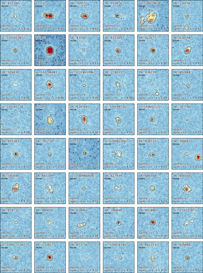
Figure B1. F814W cutouts sorted by redshift (part 1). The dashed contours show −3σ levels and the solid contours show 3σ, 5σ, 10σ, 15σ, and 30σ levels. All cutouts are 2″ on each side.
Download figure:
Standard image High-resolution image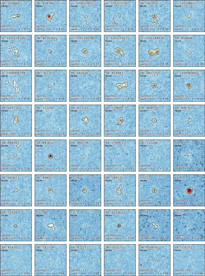
Figure B2. F814W cutouts sorted by redshift (part 2).
Download figure:
Standard image High-resolution image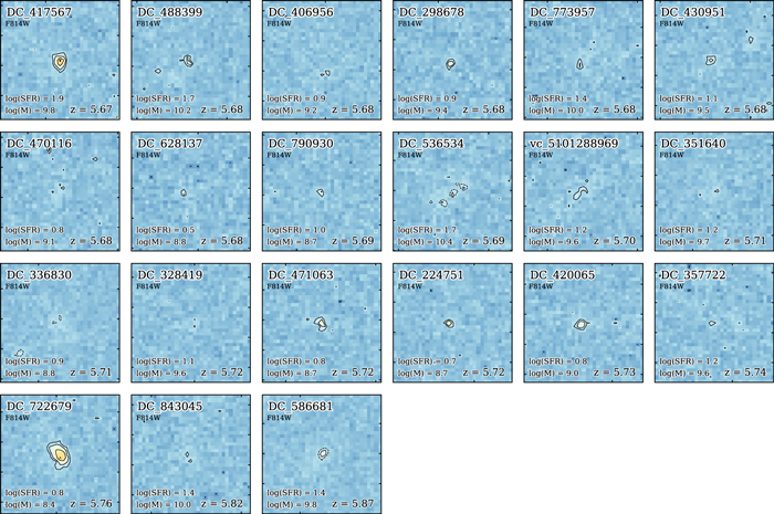
Figure B3. F814W cutouts sorted by redshift (part 3).
Download figure:
Standard image High-resolution image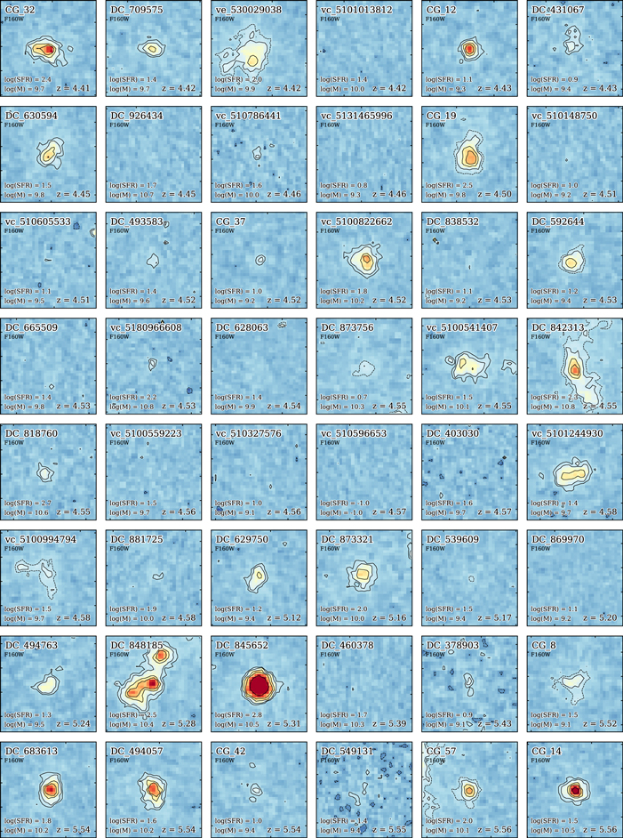
Figure B4. F160W cutouts sorted by redshift (part 1). The dashed contours show −3σ levels and the solid contours show 3σ, 5σ, 10σ, 15σ, and 30σ levels. All cutouts are 2″ on each side.
Download figure:
Standard image High-resolution image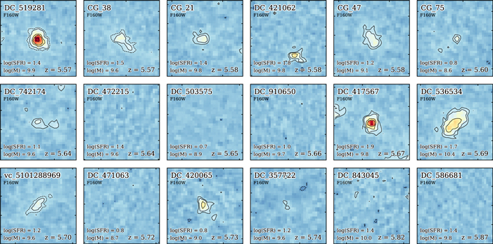
Figure B5. F160W cutouts sorted by redshift (part 2).
Download figure:
Standard image High-resolution imageFigures B6–B10 show the rest-frame UV spectra for each ALPINE galaxy sorted by increasing redshift. The spectra are smoothed with a Savitzky–Golay filter of size 2 Å. Prominent emission lines as well as individual absorption lines and absorption line complexes are indicated by the dark red bars (compare to Section 2.4.2). For some of the galaxies in COSMOS, a spectrum obtained by VUDS and Keck/DEIMOS is available. The names of these galaxies have an appended “_v” or “_d,” respectively. Note their different spectral resolution.
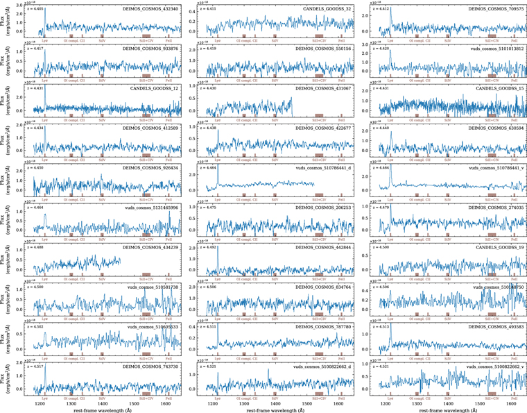
Figure B6. Rest-frame UV spectra of all galaxies sorted by redshift (part 1).
Download figure:
Standard image High-resolution image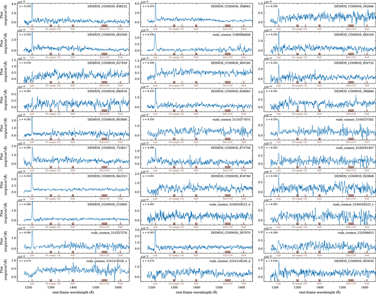
Figure B7. Rest-frame UV spectra of all galaxies sorted by redshift (part 2).
Download figure:
Standard image High-resolution image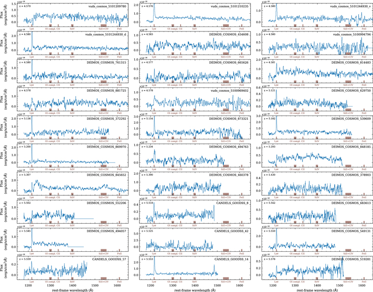
Figure B8. Rest-frame UV spectra of all galaxies sorted by redshift (part 3).
Download figure:
Standard image High-resolution image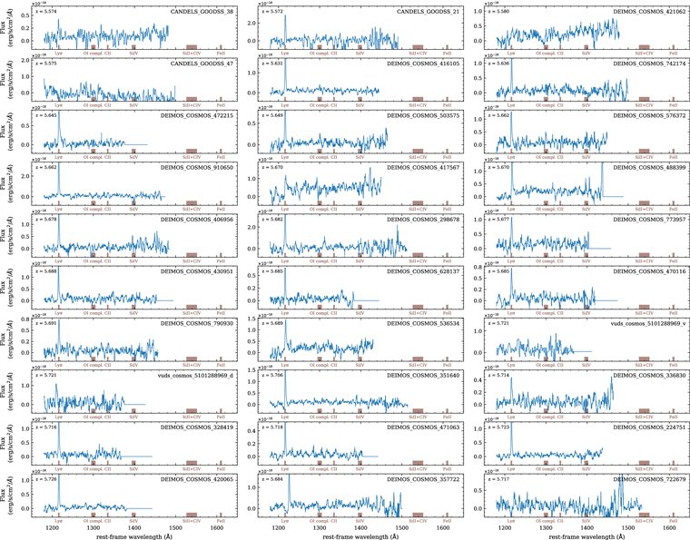
Figure B9. Rest-frame UV spectra of all galaxies sorted by redshift (part 4).
Download figure:
Standard image High-resolution image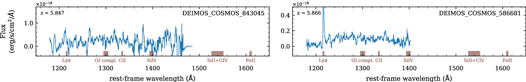
Figure B10. Rest-frame UV spectra of all galaxies sorted by redshift (part 5).
Download figure:
Standard image High-resolution imageFootnotes
- 28
- 29
One of these galaxies, ve_530029038, has also been observed by the VUDS survey.
- 30
Here, we refer to the [
] absorption line complex consisting of , , [], and . - 31
This absorption consists of two lines (1548.2 Å and 1550.8 Å) and here we give the average wavelength.
- 32
- 33
The value of this visual flag is −99 if the S/N is too low to obtain a redshift, and 1 and 2 for reliable and very reliable redshift measurements, respectively.
- 34
- 35
- 36
- 37
- 38
- 39
- 40
- 41
The photometric redshifts given in the COSMOS2015 catalog are consistent within 0.2 with our spectroscopic redshifts for more than 95% of all cases.
- 42
- 43
There is also data in the F098W filter, however, unfortunately no ALPINE galaxies are covered.
- 44
- 45
The delayed SFR is parameterized as
such that ψ(t) is maximal at t = τ. - 46
Note that the stellar masses are primarily constrained through the Spitzer photometry that covers rest-frame wavelengths redward of the Balmer break.
- 47
The f-factor,
, describes the differential dust reddening between the stellar continuum and nebular regions. Its value is largely unknown at z > 2, but it is expected that f approaches a value closer to unity at higher redshifts (Erb et al. 2006; Reddy et al. 2010; Kashino et al. 2013; Koyama et al. 2015; Valentino et al. 2015; Puglisi et al. 2016; Kashino et al. 2017; Faisst et al. 2019).