Abstract
We propose a flexible method for estimating luminosity functions (LFs) based on kernel density estimation (KDE), the most popular nonparametric density estimation approach developed in modern statistics, to overcome issues surrounding the binning of LFs. One challenge in applying KDE to LFs is how to treat the boundary bias problem, as astronomical surveys usually obtain truncated samples predominantly due to the flux-density limits of surveys. We use two solutions, the transformation KDE method ( ) and the transformation–reflection KDE method (
 ) to reduce the boundary bias. We develop a new likelihood cross-validation criterion for selecting optimal bandwidths, based on which the posterior probability distribution of the bandwidth and transformation parameters for
  and
and  are derived within a Markov Chain Monte Carlo sampling procedure. The simulation result shows that
  and
and  perform better than the traditional binning method, especially in the sparse data regime around the flux limit of a survey or at the bright end of the LF. To further improve the performance of our KDE methods, we develop the transformation–reflection adaptive KDE approach (
 ). Monte Carlo simulations suggest that it has good stability and reliability in performance, and is around an order of magnitude more accurate than using the binning method. By applying our adaptive KDE method to a quasar sample, we find that it achieves estimates comparable to the rigorous determination in a previous work, while making far fewer assumptions about the LF. The KDE method we develop has the advantages of both parametric and nonparametric methods.
1. Introduction
Redshift and luminosity (or magnitude) are undoubtedly the two most fundamental observational quantities for galaxies. As a bivariate density function of redshift and luminosity, the luminosity function (LF) provides one of the most important tools to probe the distribution and evolution of galaxies and active galactic nuclei (AGNs) over cosmic time. Measuring the LF at various wave bands has long been an important pursuit of a large body of work over the last 50 yr (e.g., Schechter 1976; Efstathiou et al. 1988; Dunlop & Peacock 1990; Boyle et al. 2000; Cole et al. 2001; Jarvis et al. 2001; Willott et al. 2001; Ueda et al. 2003; Yang et al. 2003; Richards et al. 2006; Faber et al. 2007; Aird et al. 2010; Ajello et al. 2012; Bouwens et al. 2015; Bowler et al. 2015; Yang et al. 2016; Yuan et al. 2016; Kulkarni et al. 2019; Tortorelli et al. 2020). However, accurately constructing the LF remains a challenge, as the observational selection effects (e.g., due to detection thresholds in flux density, apparent magnitude, color, surface brightness, etc.) lead to truncated samples and thus introduce bias into the LF estimation (Johnston 2011).
To date, there have been numerous statistical approaches devised to measure the LF. These mainly include parametric techniques and nonparametric methods (see Johnston 2011, for an overview). Parametric methods typically provide an analytic form for the estimated LF, where the parameters are determined either by a maximum likelihood estimator (e.g., Sandage et al. 1979; Marshall et al. 1983; Jarvis & Rawlings 2000; Willott et al. 2001; Andreon et al. 2005; Brill 2019), or within a Bayesian framework and applying a Markov Chain Monte Carlo (MCMC) algorithm (e.g., Andreon 2006; Zeng et al. 2014; Yuan et al. 2016, 2017). The parametric method can naturally incorporate various complicated selection functions and has the flexibility to be extended to trivariate LFs, for which additional quantities need to be defined, such as the photon index in the case of γ- and X-ray LFs (e.g., Ajello et al. 2012) and the spectral index for radio LFs (e.g., Jarvis & Rawlings 2000; Yuan et al. 2016), aside from luminosity and redshift. In addition, with the help of powerful statistical techniques such as the MCMC algorithm, the parametric method can be very accurate. But the premise is that we are fortunate enough to “guess” the right functional form for the LF. To reproduce the features of “observed LFs”6 of AGNs, many LF models have been proposed. These include pure density evolution (e.g., Marshall et al. 1983), pure luminosity evolution (e.g., Pei 1995; Boyle et al. 2000), luminosity-dependent density evolution (e.g., Miyaji et al. 2000; Hasinger et al. 2005), luminosity and density evolution (e.g., Aird et al. 2010; Yuan et al. 2017), and luminosity-dependent luminosity evolution (e.g., Massardi et al. 2010; Bonato et al. 2017) models. The main trend is that LF models are becoming more and more complex, with many nonphysical assumptions. This is a severe drawback for the parametric method.
Nonparametric methods are statistical techniques that make as few assumptions as possible (Wasserman et al. 2001) about the shape of the LF and derive it directly from the sample data. The explosion of data in future astrophysics studies provides unique opportunities for nonparametric methods. With large sample sizes, nonparametric methods make it possible to find subtle effects, which might be obscured by the assumptions built into parametric methods (see Wasserman et al. 2001). Common nonparametric methods include various binning methods (e.g., Schmidt 1968; Avni & Bahcall 1980; Page & Carrera 2000), the stepwise maximum likelihood method (Efstathiou et al. 1988) and the Lynden-Bell (1971)  method and its extended versions (e.g., Efron & Petrosian 1992; Caditz & Petrosian 1993). More recently, some more-rigorous statistical techniques have emerged, such as the semiparametric approach of Schafer (2007) and the Bayesian approach of Kelly et al. (2008). Each of these nonparametric methods has advantages and disadvantages.
Among the nonparametric methods, the binning method is arguably the most popular one, due to its simplicity. Although more than five decades have passed since its original version (i.e., the 1/Vmax estimator; Rowan-Robinson 1968; Schmidt 1968) was presented, binning methods are still widely used even in the most recent literature (e.g., de La Vieuville et al. 2019; Herenz et al. 2019; Kulkarni et al. 2019; Lan et al. 2019). One of the drawbacks of binning methods is that the choice of bin center and bin width can significantly distort the shape of the LF, particularly in the low number density regime. This subsequently impacts the shape of the parametric form, which is usually fit to these binned points, particularly in cases where the K corrections are nontrivial, such as the case for high-redshift galaxy samples (e.g., Bouwens et al. 2015; Bowler et al. 2015). The C− method and its variants do not Require any binning of data to estimate the cumulative distribution function of the LF. But they typically assume that luminosity and redshift are statistically independent. The semiparametric approach of Schafer (2007) is powerful and mathematically rigorous, but the sophisticated mathematics may necessitate more time for it to be recognized and put to widespread use. The Bayesian approach of Kelly et al. (2008) can be seen as a combination of parametric and nonparametric methods, where the LF is modeled as a mixture of Gaussian functions. This approach has many free parameters (typically ∼22–40) and requires critical prior information for the parameters.
Motivated by these issues, we have developed a nonparametric method based on kernel density estimation (KDE).7
KDE is a well-established nonparametric approach to estimate continuous density functions based on a sampled data set. Due to its effectiveness and flexibility, it has become the most popular method for estimation, interpolation, and visualization of probability density functions (Botev et al. 2010). In recent years, KDE has gradually been recognized by the astronomical community as an important tool to analyze data (e.g., Ferdosi et al. 2011; Hatfield et al. 2016; de Menezes et al. 2019; Trott et al. 2019). The basic idea of our KDE method is that the contribution of each data point to the LF is regarded as a smooth bump, whose shape is determined by a Gaussian kernel function  . Then, KDE sums over all these bumps to obtain a density estimator. In the analysis, the uncertainties on the measured redshifts and luminosities of the sources in the sample are ignored.
This paper is organized as follows. Section 2 gives a brief introduction to the KDE. Section 3 describes the bandwidth selection method for KDE, introduces the boundary bias problem for the LF estimate, and specifies the techniques of estimating LFs by KDE. In Section 4, the KDE methods are applied to simulated samples. Section 5 shows the result of using our KDE method in a quasar sample. Section 6 gives a comparison of our approach with previous LF estimators. The main results of this work are summarized in Section 7. Throughout this paper, we adopt a Lambda Cold Dark Matter cosmology with the parameters Ωm = 0.27, ΩΛ = 0.73, and H0 = 71 km s−1 Mpc−1.
2. Kernel Density Estimation
2.1. Definition
Let  denote a d-dimensional random vector with density f(x) defined on Rd, and let {
 } be a sequence of independent identically distributed random variables drawn from f(x). The general d-dimensional multivariate KDE of f is given by
where K( · ) is a multivariate kernel function, and H is the d × d bandwidth matrix or smoothing matrix, which is symmetric and positive definite. In this paper, we focus on the two-dimensional (2D) case.
KDE can be viewed as a weighted sum of density “bumps” that are centered at each data point  (Gramacki 2018). The shape of the bumps is determined by the kernel function K( · ), while the width and orientation of the bumps are determined by the bandwidth matrix
  . It is widely accepted that the choice of kernel function is a secondary matter in comparison with the selection of the bandwidth (e.g., Wand & Jones 1995; Botev et al. 2010; Chen 2017; Gramacki 2018). In most cases, the kernel has the form of a standard multivariate normal density given by

which is what we shall use hereafter. Choosing the form of H depends on the complexity of the underlying density (Sain 2002). Depending on the complexity, H can be isotropic, diagonal, or a full matrix, such as
The top panel of Figure 1 provides a toy example of using the KDE (assuming H is diagonal) in 10 hypothetical observations. Ellipses delineate the kernel spread one bandwidth (the semiaxes of each ellipse are h1 and h2) away from each hypothetical point. If H is isotropic, these ellipses will degenerate into circles; else, if H is a full matrix, these ellipses will also have an orientation determined by h12. Sain (2002) argued that for most densities, in particular unimodal ones, allowing different amounts of smoothing for each dimension (diagonal bandwidth matrix) is adequate. Indeed, for the problem in this work, we find that the choice of diagonal bandwidth matrix is typically sufficient. If H is diagonal, Equation (1) can be simplified to

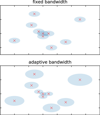
Figure 1. A toy example demonstrating the idea of the KDE with fixed and adaptive bandwidths. Ellipses delineate the kernel spread one bandwidth away from each hypothetical point (represented by red crosses).
Download figure:
Standard image High-resolution image2.2. Adaptive Kernel Density Estimation
Equation (1) assumes that the bandwidth H is constant for every individual kernel. This may lead to poor estimator performance for heterogeneous point patterns (Davies & Baddeley 2018). A popular solution to this problem is using a variable bandwidth or adaptive kernel estimator, which allows H to vary depending on the local density of the input data points (Breiman et al. 1977); a relatively small bandwidth is needed where observations are densely distributed, and a large bandwidth is required where observations are sparsely distributed (e.g., Hu et al. 2012). As a visual comparison to fixed-bandwidth estimation, the bottom panel of Figure 1 shows the kernel spread one bandwidth away from each hypothetical point for the adaptive estimator.
For the diagonal bandwidth matrix case, the bivariate adaptive kernel estimator (see Sain 2002) is given by

Abramson (1982) suggested that the bandwidths are inversely proportional to the square root of the target density itself. Obviously, the target density is unknown. According to Silverman (1986), the practical use of Abramson's (1982) approach is implemented as

where β ≡ 1/2, and  is a pilot estimate of the unknown density calculated via Equation (3) with a fixed pilot bandwidth matrix
  h10 and h20 are the overall smoothing parameters for the variable bandwidths referred to as the global bandwidths (Davies et al. 2018).
3. Estimating the Luminosity Function via KDE
3.1. The Luminosity Function
The differential LF of a sample of astrophysical objects is defined as the number of objects per unit comoving volume per unit luminosity interval,

where z denotes redshift and  denotes the luminosity. Due the typically large span of the luminosities, it is often defined in terms of
  (e.g., Cara & Lister 2008),

where  denotes the logarithm of luminosity.
In an actual survey, only a very limited number of objects in the universe can be observed, as our survey only covers a fraction of the sky and is subject to a selection function. Thus, the estimation of LFs is inevitably based on a truncated sample of objects. The integral of the LF over the survey region W should be approximately the sample size n, for sufficiently large n, i.e.,

where Ω is the solid angle subtended by the survey, and dV/dz is the differential comoving volume per unit solid angle (Hogg 1999). The LF is related to the probability distribution of (z, L) as

Once we have an estimate of p(z, L) by the KDE, we can easily convert this to an estimate of ϕ(L, z) using Equation (9). It needs to be emphasized that the domain of p(z, L) is the survey region W, thus the domain of the LF estimated by Equation (9) is also limited to W.
3.2. Optimal Bandwidth Selection for KDE
Choosing the bandwidth parameter is the most crucial issue in using KDE to estimate p(z, L), as the accuracy of KDE depends very strongly on the bandwidth matrix (e.g., Gramacki 2018). Basically, all common approaches to bandwidth selection, which measures the closeness of  to its target density f, are based on some appropriate error criteria. One of the most well-known error measurements is the mean integrated square error (MISE). The optimal bandwidth can be obtained by minimizing the Asymptotic MISE (AMISE), the dominant quantity in the MISE (Chen 2017). The three major types of bandwidth selectors include the rule of thumb, cross-validation (CV) methods, and plug-in method. In this work, we focus on the CV method, and our selector is based on the likelihood cross-validation (LCV) criterion.
3.2.1. Likelihood Cross-validation
The LCV thinks about the estimated density itself as a likelihood function, and the LCV objective function is given by
where  is the leave-one-out estimator
If H is diagonal, Equation (11) can be simplified to
The LCV bandwidth matrix  is the maximizer of the LCV(H) objective function (e.g., Davies et al. 2018)

and it has to be maximized numerically. In view of the difficult numerical procedure as the dimension of data increases, Zhang et al. (2006) improved the LCV method from a Bayesian perspective. They treated nonzero components of H as parameters, whose posterior density can be obtained using the MCMC technique based on the LCV criterion. Given H, the logarithmic likelihood function of { } is
} is
However, as pointed out by Zhang et al. (2006), when using the likelihood given by Equation (15) to perform the Bayesian inference, sufficient prior information on the components of H is required. Using this likelihood function in our problem does not lead to convergence for the MCMC algorithm; we therefore consider a new likelihood function.
3.2.2. A New LCV Method
The new candidate likelihood function is derived from Marshall et al. (1983). In their analysis, the probability distribution of the likelihood for the observables is described by Poisson probabilities. The L−z space is divided into small intervals of size dLdz. In each element, the expected number of objects at z, L is  . The likelihood function,
  , is defined as the product of the probabilities of observing one object at each (
 ) element and the probabilities of observing zero objects in all other (zj, Lj) elements in the accessible regions of the z−L plane (Marshall et al. 1983). Using Poisson probabilities, one has
Transforming to the standard expression  and dropping terms that are not model dependent, we obtain
The likelihood function given above naturally incorporates the selection function of the sample (by considering the integral interval W), and it has proved popular (Johnston 2011) and has been widely applied to the parametric estimation of LFs (e.g., Ajello et al. 2012; Yuan et al. 2016; Kulkarni et al. 2019).
Inserting Equation (9) into Equation (16) and dropping terms that are not model dependent, we obtain
Equation (17) enables one to transform the LF measurement into a problem of probability density estimation.  can be replaced with its KDE form
  given by Equation (3), and p(zi, Li) is replaced with the leave-one-out estimator
  constructed by Equation (12). Then, we have
Note that in the first term  should not be confused with
  . The term “leave one out” means that the observations used to calculate
  are independent of (zi, Li). This is where the name “cross-validation” comes from: using one subset of data to make analysis on another subset (see Gramacki 2018).
Using Equation (18), we can obtain the optimal bandwidth by minimizing S,

We find that the above bandwidth selector performs better than the LCV selector given by Equation (13). We note that the numerical optimization result of the LCV selector depends on the initial values, suggesting it may have more than one local maximum in the objective function. In this respect, our new selector has better stability.
Equation (18) can also be used to perform Bayesian inference by combining it with prior information on the bandwidths h1 and h2. We find that using uniform priors for h1 and h2 are sufficient to employ the MCMC algorithm. Therefore, our new likelihood function is a better choice than the one given by Equation (15), which requires more critical prior information.
3.3. Boundary Effects for the LF Estimate
Recall that the domain of  in Equation (9) is the survey region W. This means that the estimate of
  using KDE is based on bounded data, while certain difficulties can arise at the boundaries and near them, known as boundary effects or boundary bias (e.g., Müller & Stadtmüller 1999).
In astronomy, many surveys are flux limited. When the observation points are plotted on the L−z plane, there is a clear truncation bound (see Figure 2(a)) defined by flim(z):

where dL(z) is the luminosity distance, Flim is the survey flux limit, and K(z) represents the K correction. One has  for a power-law emission spectrum of index α (e.g., Singal et al. 2011). To give reliable results, any LF estimator must treat the truncation boundary, or flux limit of the survey, properly. From Equation (20), we can see that only when
  and α is constant is the truncation bound defined by flim(z) a curve. Otherwise, if the K correction K(z) takes a more complex form, the truncation bound will be a 2D region but not a simple curve. In this section, we only consider the simple case for the truncation boundary—a simple curve.

Figure 2. Panel (a): a simulated sample illustrates the truncation bound (red dashed line). More details about the simulation are given in Section 4. Panel (b): this shows how the simulated data in panel (a) will look like after transformation by Equation (21). Panel (c): the light gray points show the transformed data according to Equation (24), and the red points are reflection points.
Download figure:
Standard image High-resolution imageThe mathematical description for the above is that, suppose we observe n points in 2D space,  . These points are always from a bounded subset W of the plane,
  ; W is referred to as the study window (e.g., Davies et al. 2018) or survey region. Direct use of the KDE formula in W may lead to the problem of underestimating the density at boundaries. The reason for the boundary problem is that the kernels from data points near the boundary lose their full probability weight and points that lie just outside the boundary have no opportunity to contribute to the final density estimation on W (e.g., Davies et al. 2018). The boundary effect has long been recognized (Gasser & Müller 1979), and it is an import research topic in KDE study (e.g., Marron & Ruppert 1994; Hall & Park 2002; Marshall & Hazelton 2010; Maleca & Schienle 2014). The common techniques for reducing boundary effects include reflection of data (e.g., Jones 1993), transformation of data (e.g., Marron & Ruppert 1994), and boundary kernel estimators (e.g., Hall & Park 2002). For the LF estimate problems, we find that the transformation method and a method of combining transformation and reflection (Karunamuni & Alberts 2005) are able to reduce boundary effects.
3.3.1. The Transformation Method
The basic idea is as follows: take a one-to-one and continuous function g, and use the regular kernel estimator with the transformed data set  . For the LF estimate, we use the following transformation:

where flim(z) is given by Equation (20), and δ1 and δ2 are transformation parameters. Figure 2(b) provides a toy example showing how a typical flux-limited data set will look like after transformation by Equation (21).
The Jacobian matrix for the above transformation is
and  . After the transformation, the density of (x, y), denoted as
  , can be estimated from Equation (3), and its leave-one-out estimator,
  , is constructed from Equation (12). Then, by transforming back to the density of the original data set, we have
Inserting Equation (22) into (18), we obtain the negative logarithmic likelihood function S. Following Liu et al. (2011), we estimate the optimal bandwidths and transformation parameters δ1 and δ2 simultaneously. They can be estimated by numerically minimizing the object function S, or by combining with uniform priors for h1, h2, δ1, and δ2, one can also employ the MCMC algorithm to sample the bandwidth and transformation parameters simultaneously. The MCMC algorithm used in this work is “CosmoMC,” a public Fortran code of Lewis & Bridle (2002). Once we know the probability density  , the KDE of the LF is easily obtained by
3.3.2. The Transformation–Reflection Method
Introduced by Karunamuni & Alberts (2005), the transformation–reflection method was originally used for univariate data. We extend the method to the bivariate case, and extending it to the trivariate case is also possible (see Section 6.2). First, we transform the original data by

where the meaning of flim and δ1 is similar to those in Equation (21). The determinant of the Jacobian matrix for the above transformation is  . Second, we add the missing “probability mass” (e.g., Gramacki 2018) represented by the data set
  . To illustrate the above ideas, Figure 1(c) shows how a typical flux-limited data set will look after transformation and reflection. The KDE of the density of (x, y) is
The corresponding leave-one-out estimator is
Then, by transforming back to the density of the original data set, we have
Inserting Equations (27) into (18), we can obtain the likelihood function for the transformation–reflection estimator. The next steps for estimating the bandwidth and transformation parameters are similar to those described in Section 3.3.1. Finally, we can obtain the LF estimated by the transformation–reflection approach,
3.3.3. The Transformation–Reflection Adaptive KDE Approach
In Equation (25), the bandwidths h1 and h2 are constant for every individual kernel. A useful improvement is to use variable bandwidths depending on the local density of the input data points. This can be achieved using the transformation–reflection adaptive KDE ( ) approach. The
  estimator is implemented on the basis of
  , and it involves the following steps:
- 1.Employ the transformation–reflection method, and obtain the optimal bandwidths and the transformation parameter, denoted by
 , , and .
 - 2.
- 3.Let the bandwidths vary with the local density:where h10 and h20 are global bandwidths which need to be determined. Unlike Equation (5) where β ≡ 1/2, we let β be a free parameter here.
- 4.
- 5.Determine h10, h20, and β via the maximum likelihood method or the MCMC algorithm. The detailed formulas for constructing and , as well as the process for determining their parameters, can be found in Appendix A.


4. Application to Simulated Data
As an illustration of the effectiveness of our KDE methods, we apply them to a simulated data set. We use the parameterized radio luminosity function (RLF) of Yuan et al. (2017, model A) as the input LF. By choosing a flux limit of Flim = 40 mJy and setting the solid angle Ω = 0.456, we ultimately simulate a flux-limited sample of  . Our sample has the redshift and luminosity limits of (z1 = 0, z2 = 6) and
  . For these simulated radio sources, we assume a power-law emission spectrum of index
  .8
.8
4.1. The Fixed-bandwidth KDE Results
Figure 3 shows the RLFs for the simulated sample, estimated by the transformation KDE (denoted as  ) and the transformation–reflection KDE (denoted as
  ) methods at several redshifts. The optimal bandwidth and transformation parameters in our KDE methods are summarized in Table 1. Their posterior probability distributions and 2D confidence contours are given in Figure 5. The regular unimodal feature of each distribution suggests that all the parameters are very well constrained (e.g., Yan et al. 2013).

Figure 3. RLFs estimated by the  (blue solid lines) and
  (green solid lines) estimators at several redshifts, compared with the estimates (black open circles) given by the binning method of Page & Carrera (2000). The red dashed–dotted lines represent the true RLF. The vertical dashed lines mark the higher luminosity limits of the simulated survey at different redshifts.
Download figure:
Standard image High-resolution imageTable 1. Parameters of KDE for the Simulated Sample
| Method | Parameters |
|---|---|

|
|
 
|
|

|
|
 
|
|

|
  
|
 
|
|

|
Note.  is implemented on the basis of
  , and
, and  ,
,  , and
, and  inherit the parameter values of
  . Parameter errors correspond to the 68% confidence level. Parameters without an error estimate were kept fixed during the fitting stage.
Download table as: ASCIITypeset image
For comparison, the result measured by the traditional binning method (denoted as  ) of Page & Carrera (2000) is also shown. In the literature, bins are commonly chosen somewhat arbitrarily. Yuan & Wang (2013) argued that this may lead to significant bias for the LF estimates close to the flux limit (see panel (a) of Figure 4). In this work, we use the simple rule of thumb suggested by Yuan & Wang (2013) to divide bins. In panel (b) of Figure 4, we illustrate this scheme for dividing bins.
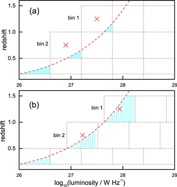
Figure 4. A toy example illustrates different schemes for dividing bins. In each panel, the red dashed line shows the flux-limit curve, the red crosses mark the centers of bins 1 and 2, and the shaded regions represent the surveyed regions in the bins. Panel (a): both the redshift and luminosity intervals are chosen arbitrarily. This may lead to the bins located at the faint end (e.g., bins 1 and 2) to contain very few objects and cause biases with small number statistics. More seriously, the binned estimator typically reports the density of a bin center as its result, but for bins 1 and 2, the bin centers are far away from the surveyed regions. In this situation, the binned LF at the faint end would be significantly biased. Panel (b): the redshift bins are chosen arbitrarily, while the starting positions of luminosity bins are determined by the intersecting points of the flux-limit curve and redshift grid lines. This dividing scheme can alleviate the faint-end bias (see Yuan & Wang 2013 for details).
Download figure:
Standard image High-resolution imageFigure 3 shows that both  and
and  are generally superior to the binning method, especially for the high-redshift (z ≥ 3) LF estimation. The KDE approaches (especially
  ) produce relatively smooth LFs, while the binning method produces discontinuous estimates, being prone to have artificial bulges and hollows.
In addition, the KDE approaches have the advantage that their measurement can be extrapolated appropriately beyond the observational limits. In Figure 3, the vertical dashed lines mark the higher luminosity limits of the simulated survey. Note that even beyond the limits, the extrapolated LFs can be a generally acceptable approximation to the true LF.
 and
and  have their own advantages and disadvantages.
  makes smother estimates, but it is prone to producing a slight negative bias at the faint end of the LFs. This is a typical boundary bias, suggesting that a simple transformation method cannot fully solve the boundary problem.
  performs well at the faint end, but not ideally at the bright end of the LFs. This is expected to be improved by using the adaptive KDE, where the data density is used.
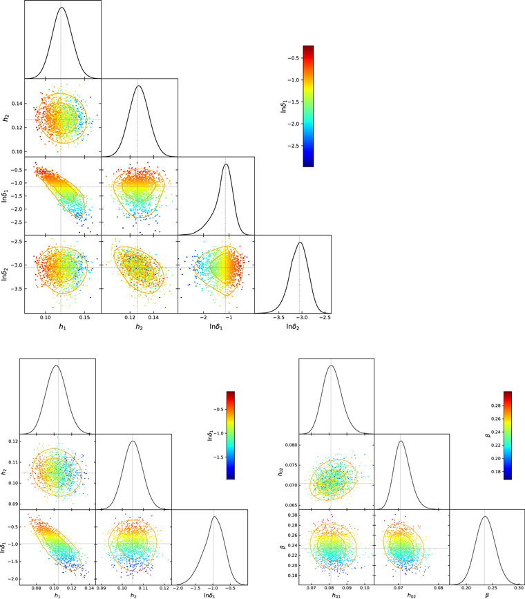
Figure 5. Marginalized 1D and 2D posterior distributions of parameters in the KDE methods. The contours containing 68% and 95% of the probability. MCMC samples are shown as colored points, where the color corresponds to the parameter shown in the color bar. The vertical lines mark the locations of the best-fit values by MCMC. The upper, lower-left, and lower-right panels correspond to  ,
,  , and
, and  respectively. The triangular plots are created by the Python package GetDist (Lewis 2019).
Download figure:
Standard image High-resolution image4.2. The Adaptive KDE Results
Figure 6 shows the RLF and its uncertainty estimated by the transformation–reflection adaptive KDE approach (denoted as  ) at several redshifts for the simulated sample. Given posterior probability distributions for the bandwidth and transformation parameters in our KDE methods (see Figure 5), the uncertainty regions of the estimated RLF are plotted by “fgivenx,” a public Python package of Handley (2018). We find that
  performs well for all six redshifts, and it achieves an excellent approximation to the true LF. Comparing with Figure 3, we notice that
  can overcome the shortcomings of
  and
and  .
.
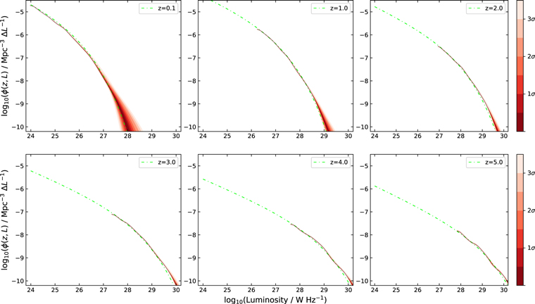
Figure 6. The RLF and its uncertainty estimated using  at several redshifts for the simulated sample. The green dashed–dotted lines represent the true RLF.
Download figure:
Standard image High-resolution imageIn order to rule out the possibility that our adaptive KDE estimator only gives a good result by chance, we simulate 200 flux-limited samples with their flux limits randomly drawn between 10−2.5 and 10−0.5 Jy. All simulated samples share the same input LF (the model A RLF of Yuan et al. 2017). By adjusting the simulated solid angle, we can control the size (n) of each sample. We let the sample size be linearly proportional to the logarithm of its flux limit. Finally, for the 200 simulated samples, their sizes are randomly distributed between 2000 and 40,000 sources.
Figures 7 and 8 shows the RLFs estimated by  and
and  , respectively, based on 200 simulated samples. Obviously, the
  estimator shows better stability and reliability in performance than the binning method. In most cases, we find that the LFs estimated by
  look like an irregular sawtooth, randomly leaping up and sloping down. This may mislead the observer to use the wrong parametric form to model the LF. Our
  estimator does not have such a drawback. In fact, this is why the KDE method is very popular in modern statistics: it can produce a smoother estimation that converges to the true density faster (Wasserman 2006).
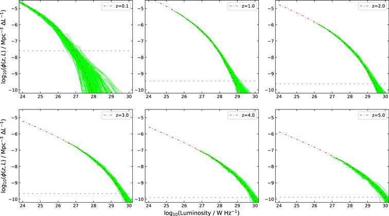
Figure 7. RLFs (green lines) estimated using  for 200 simulated samples at several redshifts. The red dashed–dotted lines represent the true RLF. The horizontal dashed lines mark the approximate observational limits of the simulated surveys, below which the RLFs are extrapolated by
  .
.
Download figure:
Standard image High-resolution image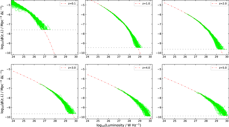
Figure 8. RLFs (green lines) estimated using  for 200 simulated samples. The red dashed–dotted lines represent the true RLF. The horizontal dashed lines mark the observational limits of the simulated surveys, below which
  cannot provide an extrapolated estimate.
Download figure:
Standard image High-resolution imageWe note that in Figure 7 the adaptive KDE method is slightly asymmetrically biased to values above the true LF compared to below the true LF (also see Figure 6), especially for the tails where LFs are extrapolated. This is because the functions of adaptive kernels given in Equation (5) only have one adjustable parameter, β, and cannot let the estimated LF go too steep too soon in the extremely low number density regime. The above effect does not matter as it is only visible for the extrapolated LFs.
4.3. Quantitative Evaluation of Performance
To quantify the performance of each LF estimator, we define a statistic dLF which measures the discrepancy of the estimated LF  from the true LF ϕ. If a large number of random vectors, denoted by {
 }
} , can be drawn from
  ,
,  can be estimated (e.g., Zhang et al. 2006) as
For the  estimator, estimates are given only at some discontinuous points, i.e., the centers of each bin. The statistic dLF is estimated by
where Nbin is the number of bins, and  locates the center of jth bin. The edges of the redshift bins are 0.0, 0.2, 0.5, 0.8, 1.2, 1.8, 2.2, 2.7, 3.3, 3.8, 4.2, 4.7, 5.3, and 6.0. The logarithmic luminosity bins are in increments of 0.3.
In Table 2, we show the statistic dLF of the different LF estimators calculated for our simulated sample. Also, the mean values  for 200 simulated samples are given. The statistic dLF of all our KDE estimators, especially
  , is significantly better than that of
  . dLF can be understood as the typical error of an LF estimator. In this sense, the
  estimator improves the accuracy by nearly an order of magnitude compared to
  . Figure 9 shows the distributions of dLF of different LF estimators for 200 simulated samples. The smaller dispersion of distributions for our KDE methods suggests that they all have significantly better stability than the
  estimator, as expected.
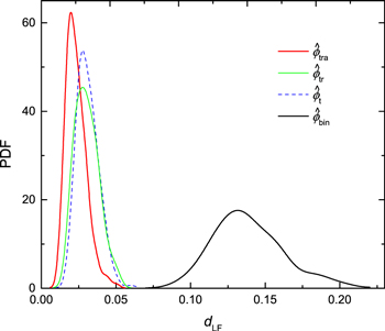
Figure 9. Distributions of dLF for different LF estimators for the 200 simulated samples. The red solid, green solid, blue dashed, and black solid curves correspond to the  ,
,  ,
,  , and
, and  estimators, respectively.
Download figure:
Standard image High-resolution imageTable 2. The Statistic dLF

|

|

|

|
|
|---|---|---|---|---|
| dLF | 0.0944 | 0.0239 | 0.0193 | 0.0157 |

|
0.1387 | 0.0311 | 0.0305 | 0.0227 |
Note. dLF is calculated for the simulated sample described in Section 4.  is the mean value for 200 simulated samples.
Download table as: ASCIITypeset image
5. Application to the Sloan Digital Sky Survey Quasar Sample
In this section, we apply our adaptive KDE method to the quasar sample of Richards et al. (2006). This sample consists of 15,343 quasars within an effective area of 1622 deg2 that was a subset of the broad-line quasar sample from Sloan Digital Sky Survey (SDSS) Data Release 3. Following Schafer (2007), we remove 62 quasars with absolute magnitude (denoted as M) > − 23.075 and 224 additional quasars that fall in an extremely poorly sampled region. After this truncation, there are 15,057 quasars remaining (see the Section 2 of Schafer 2007). In Figure 10(a), we show these quasars (light gray points) in the M −z plane as well as the truncation boundary (red dashed line). According to Richards et al. (2006), the sample was not assumed to be complete within the truncated region. Thus, each object was assigned a weight (wi; inverse of the value of the selection function) depending on its redshift and apparent magnitude. The selection function did not have an analytical form and was approximated via simulations (see Richards et al. 2006 for details).
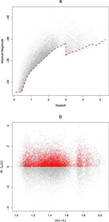
Figure 10. Panel (a): the quasar sample used in this analysis. The data are from Richards et al. (2006). The red dashed line shows the truncation boundary, defined by flim(z). Panel (b) shows how the quasar data look like after transformation (light gray points) by Equation (32), and adding the reflection points (red points).
Download figure:
Standard image High-resolution imageThe quasar LF,  , is defined by simply replacing L with M in Equation (7). To estimate the quasar LF using the transformation–reflection adaptive KDE approach, we transform the original quasar data by

where flim(z) is the function defining the truncation boundary of the quasar sample. It does not have an analytical form. Schafer (2007) provided the values of flim(z) at a series of discrete points, based on which we can calculate flim(z) using a linear interpolation. Figure 10(b) shows how the quasar data look after transformation (light gray points) and adding the reflection points (red points). There is a clear dip in the density of quasars at  , which is especially obvious after the data are transformed. This is not surprising, as the selection function is particularly low at redshift 2.7, where quasars have colors very similar to ACF stars (Richards et al. 2006). Hence, the weighting due to the selection function needs to be taken into account when using our adaptive KDE approach. The detailed formulas for considering the weighting can be found in Appendix B.
Figure 11 shows the quasar LF estimated by our transformation–reflection adaptive KDE approach (red solid lines) at several redshifts. The optimal bandwidth and transformation parameters of the KDE are summarized in Table 3. Their posterior probability distributions and 2D confidence contours are given in Figure 12. Comparisons are made with the semiparametric estimates (green lines with error bars) given in Schafer (2007) and the binned estimates (light gray circles with error bars) given in Richards et al. (2006). Our result is in good agreement with the two previous estimates. Schafer (2007) gives estimates beyond the lower luminosity limit, which can be ascribed to the assumed parametric form  used in their method. Both the Schafer (2007) method and our adaptive KDE estimator can give extrapolations of the LF beyond the higher luminosity limits, and the two results are generally consistent with each other. The ability to extrapolate LFs beyond currently observable luminosities and redshifts is very useful, as this may guide the design of future surveys (Caditz 2018). Overall, our method achieves estimates comparable to those of Schafer (2007), but makes no assumptions about the parametric form of the LF.
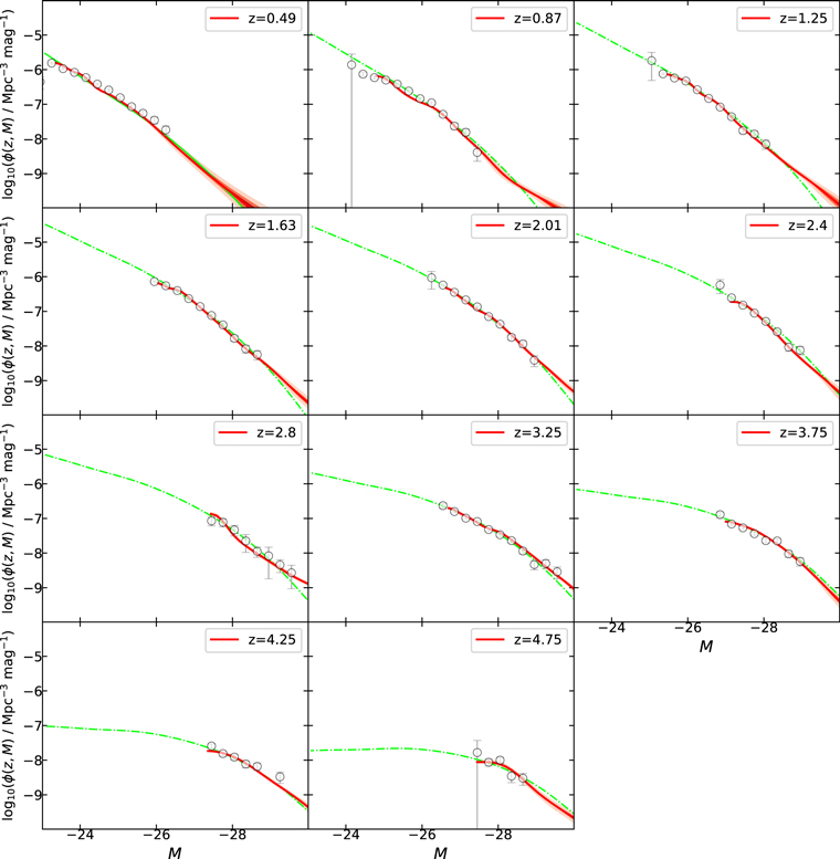
Figure 11. Quasar LF estimated by our transformation–reflection adaptive KDE approach (red solid lines) at different redshifts. The light shaded areas take into account the 3σ error bands. Comparisons are made with the semiparametric estimates (green dashed–dotted lines) given in Schafer (2007) and the binned estimates (light gray circles with error bars) given in Richards et al. (2006).
Download figure:
Standard image High-resolution image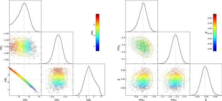
Figure 12. Marginalized 1D and 2D posterior distributions of parameters for estimating the quasar LF. The contours containing 68% and 95% of the probability. The meaning of the colored points and vertical lines are the same as those in Figure 5. The left and right panels correspond to  and
and  , respectively.
Download figure:
Standard image High-resolution imageTable 3. Parameters of KDE for the Quasar Sample
| Method | Parameters |
|---|---|

|
|
|
|

|
  
|
|
|

|
Note. Parameter errors correspond to the 68% confidence level. Parameters without an error estimate were kept fixed during the fitting stage.
Download table as: ASCIITypeset image
6. Discussion
6.1. Comparison with Previous Methods
Hitherto, the classical binned estimator ( ) is still the most popular nonparametric method. The original version of
  is the famous 1/Vmax estimator (Schmidt 1968). It was originally a variation of the V/Vmax test (Schmidt 1968), while V/Vmax is essentially a completeness estimator (see Johnston 2011). This makes it impossible for the 1/Vmax method to be a mathematically rigorous density estimator. The
  estimator cannot accurately calculate the surveyed regions for objects close to the flux limit of their parent sample and thus produces a significant systematic error (see Page & Carrera 2000; Yuan & Wang 2013). To improve the 1/Vmax estimator, Page & Carrera (2000) proposed a new method that rests on a stronger mathematical foundation. The new method is superior to the 1/Vmax estimator (e.g., Yuan & Wang 2013). For the LF at the center of a bin with luminosity interval (Lmin, Lmax) and redshift interval (zmin, zmax), the new estimator gave
where N is the number of sources detected within the bin. The double integral in Equation (33) naturally considers the truncation boundary as discussed in Section 3.3. In this text, we do not strictly distinguish among the Page & Carrera (2000) method, 1/Vmax, and 1/Va (the generalized version of 1/Vmax used for multiple samples; Avni & Bahcall 1980). They are collectively referred to as  .
.
 is widely acknowledged for its simplicity and ease of implementation. However, it has some severe drawbacks. First, its estimate depends on the division of bins but currently there are no effective rules to guide the binning. Second, it produces discontinuous estimates, and the discontinuities of the estimate are not due to the underlying LF but are only an artifact of the chosen bin locations. These discontinuities make it very difficult to grasp the structure of the data. Third, the binning of data undoubtedly leads to information loss, and potential biases can be caused by evolution within the bins. Fourth,
  is a bivariate estimator, and it cannot be properly extended to the trivariate situation. Because the number of bins grows exponentially with the number of dimensions, in higher dimensions one would require many more data points or else most of the bins would be empty (the so-called curse of dimensionality; Gramacki 2018). A trivariate LF estimator is necessary in the situation when additional quantities (such as the photon index; Ajello et al. 2012) besides the redshift and luminosity are incorporated into the LF analysis to tackle complex K corrections (see Yuan et al. 2016). In this case, there is the risk of using a low-dimensional tool to deal with higher dimensional problems. These drawbacks prevent
  from being a precise estimator. Usually, the estimates of
  are used to provide guidance or calibration for modeling the LF. If the
  result itself is not accurate, the parametric description cannot be reliable.
From a mathematical perspective, the  estimator is a kind of 2D histogram. All the drawbacks of
  are inherited from the histogram. In the mathematical community, the histogram is an outdated density estimator, used only for rapid visualization of results in one or two dimensions (e.g., Gramacki 2018). To conquer the shortcomings of histograms, mathematicians have developed some other nonparametric estimators, such as smoothing histograms, Parzen windows, k-nearest neighbors, KDE, etc. Among these, KDE is the most popular density estimator. This is why we develop the new LF estimator within a KDE framework. Our KDE methods can overcome all the drawbacks of
  and significantly improve the accuracy.
The Lynden-Bell (1971)  method, and its variants (e.g., Efron & Petrosian 1992; Caditz & Petrosian 1993), is another important estimator. It overcomes some of the shortcomings in
  . Recently, Singal et al. (2014) extended C− to the trivariate scenario and presented the redshift evolutions and distributions of the gamma-ray luminosity and photon spectral index of flat-spectrum radio quasars. This suggested that C− has good extensibility in dimension. However, the direct product of C− is the cumulative distribution function of the LF but not the LF itself, and this is inconvenient. A more serious disadvantage is that
  typically assumes that luminosity and redshift are statistically independent. In actual application, one inevitably has to introduce a parameterized model that removes the correlation of luminosities and redshifts (e.g., Singal et al. 2014).
Motivated by the potential hazards and pitfalls existing in the above traditional estimators, approaches based on more innovative statistics have been developed. One typical representative is the semiparametric approach of Schafer (2007). Schafer decomposed the bivariate density  into
into

where f(z) and g(z) are determined nonparametrically, while h(z, M, θ) has a parametric form. From Figure 11, we find that our adaptive KDE method achieves estimates comparable to those of Schafer (2007) while making far fewer assumptions about the shape of the LF. The Bayesian approach of Kelly et al. (2008) is another estimator based on innovative statistics. This method is similar to ours in some aspects, e.g., both are within a Bayesian framework and using MCMC algorithms for estimating the parameters; both model the LF as a mixture of Gaussian functions. The difference is that we arrange a relatively unified Gaussian function at each data point, and the final LF is the sum of all the Gaussian functions, while Kelly et al. (2008) use far fewer (typically ∼3–6) Gaussian functions, and each of them has six free parameters for adjusting the shape and location. Therefore, our method has much fewer (typically ∼3–6) parameters than theirs (typically ∼22–40). In addition, their method requires much more critical prior information for parameters to aid the convergence of the MCMC. Generally, they assume that the LF is unimodal, thus their prior distributions are constructed to place more probability on situations where the Gaussian functions are close together (see Figure 3 of Kelly et al. 2008). Our KDE method does not impose any preliminary assumptions on the shape of LFs, and simply use uniform (so-called “uninformative”) priors for the parameters to run the MCMC. Therefore, our method is more flexible.
6.2. Extensibility
Our KDE methods can be easily extended to the trivariate LF situation. Below we give an example for employing the  estimator in this case. Suppose we observe n objects
  within a survey region W, and
  .
.  are the single power-law spectral index, redshift, and luminosity of the ith object, respectively. Transform the observed data by

where  defines the truncation boundary of the sample and is given by

where dL(z) is the luminosity distance,  is the survey flux limit, and
  represents the K correction, where
  for a power-law emission spectrum of index α. If the emission spectrum is not a power law,
  would have a different functional form. Thus, we reserve the possibility that α can also represent other quantities to determine the K correction. In Appendix C, we give the procedure of using the transformation–reflection KDE for trivariate LFs. The adaptive KDE formulas can be easily derived.
6.3. Future Development
In mathematics, KDE is a very effective smoothing technique with many practical applications, and analysis of KDE methods is an ongoing research task. New research on bandwidth selection, reducing the boundary bias, multivariate KDE, and fast KDE algorithm for big data, etc. are continuously emerging (e.g., Cheng et al. 2019; Igarashia & Kakizawa 2019). The fast KDE algorithm is especially relevant to astronomical surveys in the near future. From Equation (1), we note that the computational complexity of KDE is of  , and it will be computationally expensive for large data sets and higher dimensions. In recent years, techniques such as using the fast Fourier transform have been proposed to accelerate the KDE computations (e.g., Gramacki & Gramacki 2017, 2017; Davies & Baddeley 2018). These ongoing developments in KDE theory mean that our LF estimator could be seen as a starting method with room to upgrade and enable it to flexibly deal with various LF-estimating problems in future surveys.
7. Summary
We summarize the important points of this work as follows.
- 1.We propose a flexible method of estimating LFs based on kernel density estimation KDE, the most popular nonparametric approach to density estimation developed in modern statistics. In view of the bandwidth selection being crucial for KDE, we develop a new likelihood cross-validation criterion for selecting the optimal bandwidth, based on the well-known likelihood function of Marshall et al. (1983).
- 2.One challenge in applying the KDE to LF estimation is how to treat the boundary bias problem, as astronomical surveys usually obtain truncated samples of objects due to observational limitations. We use two solutions, the transformation KDE method () and the transformation–reflection KDE method () to reduce the boundary bias. The posterior probability distribution of the bandwidth and transformation parameters for and are derived within an MCMC sampling procedure.
- 3.Based on an Monte Carlo simulation, we find that the performance of both and is superior to the traditional binning method.
- 4.To further improve the performance of our KDE methods, we develop the transformation–reflection adaptive KDE method (). Monte Carlo simulations show that it achieves an excellent approximation to the true LF, with good stability and reliability in performance, with accuracy of around an order of magnitude better than for the binning method.
- 5.We apply our adaptive KDE method to a quasar sample and obtain results consistent with the rigorous determination of Schafer (2007), while making far fewer assumptions about the shape of the LF.
- 6.The KDE method we develop has the advantages of both parametric and nonparametric methods. It (1) does not assume a particular parametric form for the LF; (2) does not require dividing the data into arbitrary bins, thereby reducing information loss and preventing potential biases caused by evolution within the bins; (3) produces smooth and continuous estimates; (4) utilizes the Bayesian method to maximize the exploitation of data information; and (5) is a new development but with opportunities for upgrades, giving it the flexibility to deal with various LF-estimating problems in the future surveys.


We thank the anonymous reviewer for the many comments and suggestions, leading to a clearer description of these results. We acknowledge the financial support from the National Natural Science Foundation of China (grant Nos. 11603066, U1738124, 11573060, and 11661161010) and Yunnan Natural Science Foundation (Nos. 2019FB008 and 2019FB009). We would like to thank Xibin Zhang, Xiaolin Yang, Dahai Yan, Xian Hou, Ming Zhou, and Guobao Zhang for useful discussions. M.J.J. acknowledges support from the Oxford Hintze Centre for Astrophysical Surveys, which is funded through generous support from the Hintze Family Charitable Foundation. The authors gratefully acknowledge the computing time granted by the Yunnan Observatories and provided on the facilities at the Yunnan Observatories Supercomputing Platform.
Software: BivTrunc (Schafer 2007), CosmoMC (Lewis & Bridle 2002), emcee (Foreman-Mackey et al. 2013), fgivenx (Handley 2018), GetDist (Lewis 2019), QUADPACK (Piessens et al. 1983).
Appendix A: The Transformation–Reflection Adaptive KDE Method
The transformation–reflection adaptive KDE is

where  and
and  are calculated via Equation (29). The leave-one-out estimator is
Then, by transforming back to the density of the original data set, we have
and,

Inserting Equations (A3) into Equation (18), we can obtain the likelihood function for the transformation–reflection adaptive KDE estimator:

where  and
and  are the redshift and luminosity limits of the simulated sample. By numerically minimizing the object function S, we can determine the optimal values for h10, h20, and β. Alternatively, by combining with uniform priors for h10, h20, and β, one can employ the MCMC algorithm to perform Bayesian inference. Finally, we obtain the LF estimated using the transformation–reflection adaptive KDE approach,

Appendix B: The KDE Method Considering the Weighting Due to the Selection Function
For the ith object in the quasar sample, with a redshift of zi and absolute magnitude of Mi, its weight is wi. The value of the weight is the inverse of the selection function for the data pair (zi, Mi). Intuitively, an object with a selection function of 0.5 is “like” two observations at that location (Richards et al. 2006). For the values of wi, we use the calculation by “BivTrunc,” a public R wrapper of Schafer (2007). To obtain  , one needs to first employ the transformation–reflection method. After transforming the original data using Equation (32), the KDE to the new data set is

where  is the effective sample size given by
  . The corresponding leave-one-out estimator is

The likelihood function for the transformation–reflection KDE estimator is

where z1 = 0.1, z2 = 5.3, and M1 = − 30.7.  and
and  are constructed similarly to Equation (27). By numerically minimizing the object function S, we can obtain the optimal bandwidths and the transformation parameters
  ,
,  , and
, and  . Then, we follow the steps introduced in Section 3.3.3 to achieve the adaptive KDE. Only the weight needs to be involved, and the new equation is

where  and
and  are calculated via Equation (29). The leave-one-out estimator is

Referring to Equations (A4) and (B3), it is easy to obtain the weighted version of the likelihood function for the  estimator. Finally, we obtain the quasar LF estimated by the
  estimator,

Appendix C: The Transformation–Reflection KDE for Trivariate LFs
After transforming the original data via Equation (35), the KDE of the density of the new data ( ) is
) is

The corresponding leave-one-out estimator is

The determinant of the Jacobian matrix for the transformation by Equation (35) is  . Thus, by transforming back to the density of the original data set, we have

and,

Inserting Equations (C3) into Equation (18), we can obtain the likelihood function:

where  ,
,  , and
, and  are the spectral index, redshift, and luminosity limits of the sample. Finally, we can obtain the trivariate LF estimated using the transformation–reflection approach,

Usually, we are more interested in the bivariate LF, and it can be obtained by

Footnotes
- 6
The so-called “observed LFs” are actually nonparametric LFs estimated using the classical binning method such as the
estimator. - 7
The code for performing the KDE analysis in this work is available upon request from Z. Yuan. A general-purpose code for KDE LF analysis will be made available on https://github.com/yuanzunli.
- 8
Strictly speaking, the spectral indexes of a sample should be a distribution rather than a single value. Nevertheless, for the steep-spectrum radio sources, the dispersion of their spectral index distribution is relatively small. Taking an average value of α = 0.75 is a safe approximation, where
.

