Abstract
Wave optics is essential for analyzing lensed gravitational waves, yet evaluating the diffraction integral F(ω, y) is computationally expensive. We present a Sinusoidal Representation Networks (SIRENs) framework for the dimensionless amplification factor, demonstrating its efficacy and generalization through point mass lens and singular isothermal sphere test cases. Unlike standard architectures that suffer from spectral bias, the network’s periodic activation functions structurally align with the integral’s oscillatory kernel, effectively resolving high-frequency spectral features. The resulting estimator achieves  relative accuracy and a ∼100× speedup compared to direct numerical integration. By shifting the computational burden to offline training, our framework yields a stable
  inference complexity. This guarantees constant, sub-millisecond evaluation times, even in the weak-lensing diffraction tail where traditional methods stagnate. Additionally, the dimensionless formulation ensures intrinsic scale invariance, enabling direct application across astrophysical regimes from stellar-mass lenses in the ground-based LIGO/Virgo/KAGRA (LVK) band to supermassive black holes in the space-based LISA band.
Original content from this work may be used under the terms of the Creative Commons Attribution 4.0 licence. Any further distribution of this work must maintain attribution to the author(s) and the title of the work, journal citation and DOI.
1. Introduction
Gravitational lensing of gravitational waves (GWs) provides a new probe for compact objects and small-scale structure that are difficult to access electromagnetically. When the GW wavelength becomes comparable to the characteristic scale of the lens, diffraction and interference produce frequency-dependent modulations in the observed signal, known as the wave-optics regime (S. Deguchi & W. D. Watson 1986; T. T. Nakamura 1998; R. Takahashi & T. Nakamura 2003). Such signatures are expected from stellar-mass black holes, compact dark matter substructure, and intermediate-mass black holes (IMBHs) lensing, and they are relevant to both the current LIGO/Virgo/KAGRA (LVK; B. P. Abbott et al. 2020) ground-based detector network (F. Acernese et al. 2014; J. Aasi et al. 2015; KAGRA Collaboration et al. 2019) and future space missions LISA (P. Amaro-Seoane et al. 2017), Taiji (Z. Luo et al. 2021), and TianQin (J. Luo et al. 2016). Within the ground-based GW detector band, we focus on lensed GWs from compact-binary coalescences (CBCs). In parts of this parameter space, the geometric-optics approximation remains adequate, e.g., ∼100 M⊙. Point mass lens (PML) can be well described by geometric optics for typical LIGO-band signals (A. Liu et al. 2023). On the other hand, wave-optics effects become relevant near the diffraction-interference transition (S. Refsdal & J. Surdej 1994; T. T. Nakamura 1998; R. Takahashi & T. Nakamura 2003; P. Christian et al. 2018; K.-H. Lai et al. 2018; K. Liao et al. 2018; G. Pagano et al. 2020; M. Oguri & R. Takahashi 2022; E. Seo et al. 2022; M. Wright & M. Hendry 2022; S. Basak et al. 2022; A. Liu et al. 2023; G. Tambalo et al. 2023a). This effect becomes nonnegligible for lens masses ML ≲ 103 M⊙ within the LVK sensitivity band (∼20–1000 Hz) and likewise within the planned space-based detector LISA band (∼10−4–1 Hz; P. Amaro-Seoane et al. 2017). Meanwhile, LVK searches in the O3 data have reported no confident lensed GW detections, highlighting the requirement for accurate and fast-forward models of lensed GWs to enable the exhaustive parameter scans (R. Abbott et al. 2021, 2024; LIGO Scientific Collaboration et al. 2025).
Recent studies have clarified the phenomenology across strong lensing and microlensing, developed fast evaluators for wave-optics amplification, and highlighted astrophysical applications (P. Christian et al. 2018; K.-H. Lai et al. 2018; K. Liao et al. 2018; G. Pagano et al. 2020; K. Kim et al. 2021; S. Basak et al. 2022; O. Bulashenko & H. Ubach 2022; M. Oguri & R. Takahashi 2022; E. Seo et al. 2022; M. Wright & M. Hendry 2022; G. Tambalo et al. 2023a). In the wave-optics regime, lensing is encoded by a complex amplification factor F(ω, y) that maps the unlensed strain to the lensed one as a function of angular frequency ω and the dimensionless source-lens offset y (in units of the Einstein radius). Even for the analytically tractable PML (S. Deguchi & W. D. Watson 1986), F(ω, y) exhibits highly oscillatory structure, particularly at moderate-to-large y, which makes direct evaluation via special functions or diffraction integrals computationally demanding. Considerable effort has been devoted to optimizing these numerical integrations. For instance, X. Guo & Y. Lu (2020) investigated the convergence of diffraction integrals and proposed a refined method combining zero-point integration with asymptotic expansions (AEs) to improve both accuracy and efficiency. Despite these improvements, direct numerical integration remains too slow for real-time generation of waveforms in large-scale parameter estimation pipelines, which may require  likelihood evaluations per event (R. J. Smith et al. 2020).
Consequently, recent efforts have focused on bypassing these computational bottlenecks through optimized numerical codes, such as GLoW (H. Villarrubia-Rojo et al. 2025) and wolensing (S. Yeung et al. 2024). However, existing surrogate paradigms face distinct limitations. Likelihood-free tools like conditional variational autoencoders (R. B. Nerin et al. 2025) estimate posteriors directly but bypass the amplification factor entirely, precluding explicit waveform evaluation. Alternatively, time-domain emulators using reduced basis methods (U. Deka et al. 2025) introduce computational bottlenecks during frequency-domain transformation and require complex manual interventions to handle singularities. While direct frequency-domain deep learning offers a fully automated alternative, standard architectures like multilayer perceptrons (MLPs) suffer from spectral bias (N. Rahaman et al. 2018), failing to resolve the dense high-frequency interference fringes characteristic of wave optics.
In this work, we employ sinusoidal representation networks (SIRENs; V. Sitzmann et al. 2020) to directly model the amplification factor F(ω, y) in the frequency domain. While neural networks are inherently “black box” models, the specific architectural choice of SIRENs provides an essential advantage: Their periodic activation functions possess a structural correspondence that is mathematically isomorphic to the oscillatory nature of the diffraction integral. This allows us to circumvent the spectral bias and accurately resolve dense interference fringes without determining time-domain counterparts. To demonstrate the efficacy of our approach, we focus on the phenomenologically rich transition zone of the wave-optics regime. This domain spans from the diffraction-dominated limit to the regime of significant interference (R. Takahashi & T. Nakamura 2003; T. T. Nakamura 1998), representing a critical benchmark where the complex, dense oscillatory fringes render traditional geometric-optics approximations inaccurate (A. Liu et al. 2023). This regime requires full wave-optics calculations, making it an ideal benchmark for validation. Furthermore, the model’s dimensionless formulation ensures scale invariance. This property allows the model to generalize to other astrophysical systems, such as supermassive black hole lenses in the LISA band.
The resulting emulator achieves subpercent accuracy across the training domain while preserving high-frequency interference features, yielding large speedups relative to direct evaluations. We take the PML as our baseline model, but we also extend the approach to more realistic lenses such as the singular isothermal sphere (SIS). In addition, we discuss the astrophysical relevance of the parameter ranges, including stellar-mass lenses and IMBH or halo substructure in space-based observations (G. Pagano et al. 2020; M. Wright & M. Hendry 2022; G. Tambalo et al. 2023b). The implementation is available at Github.6
This paper is organized as follows: In Section 2, we review the theoretical framework of wave-optics lensing for the PML model. Section 3 provides an overview of traditional numerical integration techniques and introduces our proposed SIREN-based architecture, supported by a theoretical analysis of its spectral properties. Section 4 outlines the experimental setup, detailing the data generation process and our physics-informed domain decomposition strategy. Section 5 presents an indepth performance evaluation, including accuracy benchmarks, computational efficiency comparisons against asymptotic-expansion methods, and a validation of the model’s generalization capability on the SIS profile. Finally, Section 6 summarizes our findings and discusses future applications. In this work, we adopt the ΛCDM cosmology model described by the Planck Collaboration (2020), which is also coded by Astropy7 (Astropy Collaboration 2022) with assumptions of H0 = 67.66 km s−1 Mpc−1, Ωm = 0.30966, and TCMB = 2.7255 K.
2. Theoretical Background: Gravitational Lensing of PML
As motivated in the Introduction, we adopt the PML as the baseline for CBCs in the LVK band, and work with the complex amplification factor F(ω, y).
2.1. Diffraction Integral Formulation
We adopt the standard geometric configuration for gravitational lensing under the thin-lens approximation, as illustrated schematically in Figure 1. A GW signal emitted by a source S at a true angular position β is deflected by a lens mass before reaching the observer. Due to this deflection, the observer perceives the signal coming from an apparent angular position θ. As shown in Figure 1, these angular positions correspond to physical coordinate vectors  in the source plane and
  (the impact parameter) in the lens plane, respectively. The system is characterized by the angular diameter distances from the observer to the lens DL, to the source DS, and between the lens and the source DLS.
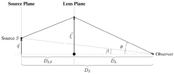
Figure 1. Schematic illustration of the thin-lens gravitational lensing geometry. The true source angular position β corresponds to vector  in the source plane, while the observed angular position θ corresponds to the impact vector
  in the lens plane. DL, DS, and DLS denote the relevant angular diameter distances to the lens and source planes.
Download figure:
Standard image High-resolution imageFollowing P. Christian et al. (2018), we define the normalized coordinates in the lens plane  , source plane
  , and observer plane
  by the Einstein radius ξ0,

where  ,
,  , and
, and  represent the physical position vectors in the lens, source, and observer planes, respectively. The Einstein radius ξ0 serves as the natural length scale.
The amplification factor F(ω, y), defined as the ratio of the lensed and unlensed GW amplitudes, is computed by solving the Fresnel–Kirchhoff diffraction integral in the thin-lens approximation,

where  is the time delay function. And the dimensionless frequency ω, related to the physical frequency f, is given by

where  is the angular frequency of the GW.
2.2. Amplification Factor for PML
The amplification factor for a PML can be derived by solving the diffraction integral, leading to the following closed-form expression for F(ω, y) (R. Takahashi & T. Nakamura 2003; P. Christian et al. 2018),
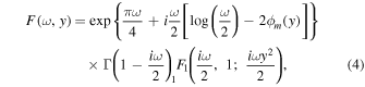
where 1F1(a, b, z) is the confluent hypergeometric function of the first kind and Γ is the Gamma function. The term ϕm(y) represents the minimum time delay and is defined by

Here xm is the position in the lens plane where the time delay is minimized, and y is the dimensionless source-lens separation in units of the Einstein radius.
For a PML, ω in Equation (3) can be written as

where ML is the mass of point lens and zL is the lens redshift. This frequency is widely used as the standard parameter to distinguish the wave-optics and geometric-optics regimes. If ω ≫ 1, under this situation the geometric-optics approximation is applicable. If the dimensionless frequency w does not satisfy this condition, the full diffraction integral incorporating wave-optics effects should be evaluated. Stellar-mass black holes can serve as representative lens objects in the PML model. For a lens mass of ML = 60 M⊙ at a redshift zL = 1, and considering the most sensitive frequency band (10–1000 Hz) of current ground-based GW detectors, the corresponding dimensionless frequency range computed using Equation (6) is w ∈ [0.15, 14.85]. In this regime, the geometric-optics approximation may not be sufficient. For PML with smaller masses or located at lower redshifts, the upper bound of w becomes even smaller, further emphasizing the necessity of computing the full amplification factor that includes wave-optics effects.
These expressions provides a detailed description of the amplification factor for lensed GWs and serves as the reference model for this study. The complex nature of F(ω, y), particularly its highly oscillatory behavior at large y, highlights the need for accurate numerical methods or machine learning–based approximations to efficiently model this function.
2.3. Physical Interpretation and Illustrative Behavior
The amplification factor F(ω, y) depends critically on two dimensionless inputs: frequency ω and impact parameter y. In the low-frequency limit (ω < 1), diffraction effects dominate and F approaches unity with a smooth envelope. As ω increases, interference fringes appear and become more closely spaced, reflecting rapid phase accumulation between multiple propagation paths. Similarly, small y values (near alignment) produce strong magnification peaks at low frequency, while larger y values weaken the overall amplitude but generate high-frequency, dense oscillations as path-length differences grow.
To visualize the characteristic behavior of the amplification factor in the wave-optics regime, we present a representative case in Figure 2 with a dimensionless impact parameter y = 1.0. In this figure, interference fringes are clearly resolved. We fix the lens redshift at zL = 0.25 and consider a lens mass of ML = 30 M⊙. According to Equation (6), the dimensionless frequency range will be ω ∈ [0.006, 10], mapping to a physical frequency band of f = [1.4 Hz, 2.2 kHz], which effectively covers the sensitivity window of ground-based GW detectors. As illustrated in Figure 2, the resulting amplification factor ∣F(ω, y)∣ exhibits highly nonstationary behavior: The oscillation frequency increases with ω, reflecting the rapid phase accumulation between interfering paths, while the amplitude modulation follows a slow envelope. The pattern is neither strictly periodic nor purely sinusoidal, and each extremum features a sharp peak. This multiscale structure, which combines a broad diffractive envelope with dense, high-frequency fringes, poses a severe challenge for low-order basis expansions or naive interpolation. This complexity motivates our adoption of a learning model capable of capturing both global trends and fine-grained spectral features.
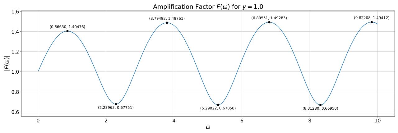
Figure 2. Illustration of ∣F(ω, y)∣ for ω ∈ [0.006, 10] at y = 1.0. This impact parameter corresponds to the Einstein radius, serving as a representative intermediate position where interference fringes are clearly visible. For a fiducial lens configuration with ML = 30 M⊙ and zL = 0.25, this ω range maps to a physical band of 1.4 Hz to 2.2 kHz, effectively covering the 10–1000 Hz sensitivity window of ground-based GW detectors. The nonperiodic, sharply pointed oscillations highlight the necessity for a model capable of capturing multiscale interference patterns.
Download figure:
Standard image High-resolution image3. Numerical Methods Overview and Model
In this section, we first review several established numerical techniques (Section 3.1) to establish a baseline; then we introduce our SIREN-based model (Section 3.2), which leverages learned high-frequency bases to achieve subpercent accuracy with dramatically reduced runtime.
3.1. Traditional Numerical Methods
Following standard wave-optics treatments (X. Guo & Y. Lu 2020), the amplification factor for an axisymmetric PML can be written as
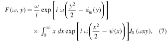
where J0 is the Bessel function of the first kind. For the definitions of other variables, including the dimensionless frequency ω, the impact parameter y, and the lens potential, we refer the reader to Section 2. Substituting z = x2/2, the diffraction integral transforms to

and  .
.
3.1.1. Integral Mean Method
We approximate the improper integral (8) by its (C, 1) Cesàro mean,

which damps late-time oscillations and converges in the mean as b → ∞.
3.1.2. Asymptotic Expansion Method
Split the domain at a finite cutoff b and write the integrand as eiωzf(z), where

Repeated integration by parts on the tail [b, ∞) leads to the asymptotic-expansion estimator

where N is the truncation order and f (n−1)(b) denotes the (n − 1)th derivative of f at z = b.
3.1.3. Levin’s Method
Levin’s method computes oscillatory integrals on a finite interval,

where f(z) is a nonoscillatory amplitude and q(z) is a smooth phase. Choose n smooth, linearly independent basis functions  and collocation nodes
 ![${\{{z}_{j}\}}_{j=1}^{n}\subset [a,b]$](https://content.cld.iop.org/journals/0067-0049/284/2/48/revision1/apjsae64e4ieqn18.gif) . The coefficients
. The coefficients  are determined by the collocation system

The collocated antiderivative yields the endpoint expression

We approximate the finite-interval integral by I(b) ≈ In(b). In our setting the integration variable is z = x2/2 with domain [0, ∞), so we set a = 0 and q(z) = ωz. Sending b → ∞ and assuming the endpoint term at b vanishes, we obtain

3.1.4. Zero-points Integral Method
Define the partial integral

Let jk be the kth positive root of J0. Under z = x2/2,


Evaluating (16) at b = zk gives

The improper integral is

A (C, 1) Cesàro average often accelerates convergence:

3.1.5. Zero-points Asymptotic Expansion Method


3.2. SIREN-based Neural Network Model
The wave-optics amplification factor F(ω, y) is characterized by intense oscillatory behavior, where dense interference fringes modulate a diffractive envelope. Numerically, direct evaluation of Equation (4) is hindered by high computational costs and instability arising from the cancellation of special-function terms in destructive-interference intervals. From a deep learning perspective, standard MLPs are also ill-suited for this task, as they suffer from spectral bias—a phenomenon where networks prioritize low-frequency features and fail to resolve rapid variations (N. Rahaman et al. 2018). In fact, our empirical tests also confirmed that standard MLPs completely fail to handle this highly oscillatory task. To overcome this limitation, we implement a coordinate-based neural network that integrates Fourier feature mappings (M. Tancik et al. 2020) with SIRENs (see Figure 3).
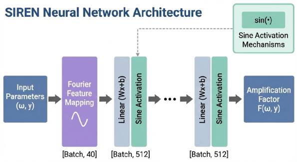
Figure 3. Architecture of the proposed neural model. The continuous input coordinates, representing the dimensionless GW frequency ω and the source-lens impact parameter y, are first projected onto a high-dimensional manifold via a fixed Gaussian Fourier feature mapping. The embedded features are then processed by a deep SIREN, where each layer employs a periodic sine activation function to naturally capture the multiscale oscillatory behavior of the amplification factor.
Download figure:
Standard image High-resolution image3.2.1. Fourier Feature Mapping
Before entering the network, the low-dimensional input coordinates x = (ω, y) are projected into a higher-dimensional feature space using a Fourier feature mapping  . This mapping enables the network to learn high-frequency functions more efficiently by controlling the spectral decay of the neural tangent kernel (NTK; M. Tancik et al. 2020). Specifically, we employ a Gaussian random Fourier feature mapping defined as

where  is a fixed weight matrix containing m sampled frequency vectors, with entries sampled from a Gaussian distribution
  . This projection maps the input onto a periodic manifold, enriching the input representation with high-frequency components prior to the learnable layers.
3.2.2. Sinusoidal Representation Network
The embedded features z0 = γ(x) serve as the input to the SIREN backbone. Unlike standard MLPs, SIREN employs a periodic sine activation function  for every hidden layer. The network operation is defined recursively as

followed by a final linear transformation zL = WLzL−1 + bL to output the real and imaginary parts of the amplification factor. Here ω0 is a hyperparameter that dictates the frequency of the activation function.
The periodic nature of the activation function provides a strong structural consistency suited for wave physics, allowing the network to represent derivatives and fine-grained structures accurately. To ensure stable signal propagation, we adopt the specialized initialization scheme proposed by V. Sitzmann et al. (2020). For the first hidden layer (accepting the Fourier features), weights are initialized from a uniform distribution,

where din is the dimensionality of the input Fourier features (i.e., 2m). For subsequent layers, weights are initialized to preserve the activation variance,

where nh denotes the number of neurons in the hidden layers. This initialization strategy prevents the gradients from vanishing or exploding, enabling the training of deep architectures capable of resolving the complex interference patterns of F(ω, y).
3.3. Theoretical Motivation of the Architecture
We employ the NTK (A. Jacot et al. 2018) to analyze the training dynamics, characterizing the convergence rate of neural networks in the frequency domain. First, consider the spectral properties of the target function. As shown in Equation (7), the amplification factor F(ω, y) is composed of a rapidly oscillating exponential prefactor and a Bessel-weighted diffraction integral. In the wave-optics regime (large ω and y), the local oscillation frequency is determined by the gradient of the phase terms. Specifically, the characteristic bandwidth νtarget is proportional to the product of the physical parameters:

This implies that the spectral support of F(ω, y) extends to high frequencies, requiring the model to resolve fine-scale variations.
Next, consider the learning process. For a network f(x;θ) trained by gradient descent, the training dynamics in the infinite-width limit decouple into independent eigenmodes of the NTK. The error decay for a specific eigenmode is governed by its eigenvalue λν,

where  is the error component corresponding to the spectral frequency ν of the target function’s decomposition (i.e., the spatial frequency in the parameter space (ω, y)), η is the learning rate, and λν determines the convergence rate. Note that ν here characterizes the rate of variation of the function F with respect to its inputs, distinct from the physical GW frequency ω, which serves as an input coordinate.
For standard MLPs with rectified linear unit (ReLU) activation, N. Rahaman et al. (2018) demonstrated that the NTK eigenvalues decay rapidly according to a power law, typically  . This induces a “spectral bias”: For the high-frequency modes present in the wave-optics regime (large νtarget), the convergence speed
  becomes negligibly small. Consequently, ReLU networks act as low-pass filters, effectively smoothing out the essential interference fringes.
In contrast, SIREN employs periodic activations  . The NTK spectrum of SIREN is not concentrated at zero but exhibits tunable bandwidth controlled by the initialization frequency ω0. By setting ω0 to match the characteristic scale of the diffraction integral, we ensure that λν remains significant across the target spectrum. Structurally, the composition of sinusoidal layers synthesizes a function:

This form is structurally analogous to the oscillatory nature of Equation (7). The correspondence between the network’s spectral properties and the physical model ensures the accurate representation of fine-grained diffraction patterns.
4. Model Implementation and Experimental Setup
The simulation workflow integrates data generation and SIREN training, as illustrated in Figure 4. This pipeline integrates the precise analytical generation of training data, the feature encoding strategy, the training of the SIREN, and the subsequent validation in the frequency domain.
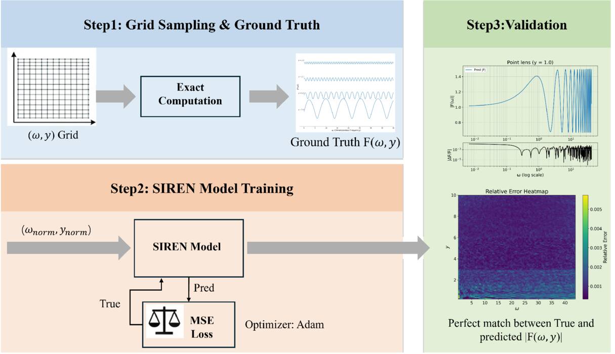
Figure 4. Computational framework for diffraction integral evaluation. The workflow proceeds in three logical steps. First, Data Generation utilizes mpmath for high-precision analytical evaluation of the amplification factor F(ω, y) on a dense grid. The selected grid astrophysically encompasses the transition from strong lensing to the weak-lensing diffraction tail, mapping universally to both stellar-mass lenses in ground-based detector bands and supermassive black holes in the LISA band. Second, Model Training employs a SIREN network enhanced with Fourier feature embeddings to learn the continuous mapping from normalized parameters to the complex amplification factor. Third, Validation compares the predicted spectral response ∣F(ω)∣ against the ground truth to ensure accurate capture of high-frequency interference patterns.
Download figure:
Standard image High-resolution image4.1. Parameter Range Selection
The choice of the input domains for ω and y is dictated by both the physical behavior of the amplification factor F(ω, y) and numerical stability considerations.
We select three representative masses of the PML ML = {10, 30, 50} M⊙, which target the stellar-mass black hole population routinely inferred in LVK catalogs. These values are used solely to determine the physically relevant boundary limits of the dimensionless frequency ω in the LVK sensitivity band, rather than to fix the lens mass during training. Based on the optimal sensitivity band of current GW detectors (advanced LVK), we select a frequency range of f ∈ [1, 1000] Hz, corresponding to the typical GW frequencies emitted by CBCs.
Throughout, we convert this physical range to the dimensionless frequency ω using Equation (6). Taking the union of these resulting intervals yields our final training domain,

where  and
and  . The model is trained directly on F(ω, y), so the dependence on ML is fully encoded through ω, and no mass-specific training is required. This range is critical as it covers the transition from the diffraction-dominated regime to the dense oscillatory fringes of the wave-optics limit.
It is worth noting that due to the scale invariance of the dimensionless formulation, this domain is astrophysically universal. Focusing on the prime LISA frequency band of f ∈ [10−4, 10−1] Hz (P. Amaro-Seoane et al. 2017), we consider the redshifted lens mass MLz = (1 + zL)ML as the primary physical parameter. In this context, our training domain of ω ∈ [0.0067, 43.93] is astrophysically versatile, as it effectively encompasses the diffraction patterns produced by MLz ranging from ∼103 M⊙ to ∼107 M⊙. Thus our selected parameter space provides a rigorous testbed applicable to a wide range of supermassive black hole lensing scenarios.
For the impact parameter y, we set

with  and
and  . The lower bound avoids numerical instability in the analytic formula as y → 0, while the upper bound extends to the weak-lensing regime where F ≈ 1. Our primary focus for detection prospects lies in the high-magnification region y ≤ 3.
4.2. Training Dataset Construction
The analytic amplification factor F(ω, y) (Equation (4)) was evaluated on a dense Cartesian grid covering the selected domain. Special-function computations were carried out using the mpmath library with global precision set to 50 decimal places. The resulting ground-truth labels were validated against adaptive quadrature of the Fresnel diffraction integral and geometric-optics limits, achieving agreement within 10−15.
4.3. Feature Encoding
Prior to network ingestion, the input coordinates (ω, y) are first normalized to the range [−1, 1] via linear scaling:

Let x = (ωnorm, ynorm). As detailed in the model architecture (Section 3.2), we enrich the input representation using a Gaussian Fourier feature mapping. In this implementation, we set the mapping dimension to m = 20 and the Gaussian scale to σ = 10.0. The resulting projected features  are concatenated with the normalized inputs x to form the final input vector passed to the SIREN backbone.
4.4. Domain Decomposition and Sampling Strategy
The amplification factor exhibits highly nonstationary behavior: Smooth variations at low y and rapid, dense oscillations at high y. This behavior poses a multiscale challenge for unified modeling. Inspired by the “Frequency Principle” (Z.-Q. J. Xu et al. 2020), which states that neural networks tend to fit low-frequency components first, we adopt a domain decomposition strategy to reduce the spectral dynamic range of each subtask. Analogous to the adaptive integration intervals employed by X. Guo & Y. Lu (2020) for numerical integration, we decompose the y-domain into four overlapping intervals ![${{ \mathcal I }}_{i}=[{\alpha }_{i},{\alpha }_{i+1}]$](https://content.cld.iop.org/journals/0067-0049/284/2/48/revision1/apjsae64e4ieqn33.gif) defined by breakpoints {0.2, 1.0, 3.0, 6.0, 10.0}.
defined by breakpoints {0.2, 1.0, 3.0, 6.0, 10.0}.
We employ a domain decomposition based on the interference characteristics:  and
and  cover the strong-lensing and high-contrast fringe regimes relevant to CBCs, while
  and
and  handle the high-frequency saturation and weak-lensing tails. This allows us to tune the network bandwidth according to local oscillatory characteristics, preventing optimization stagnation common in single networks facing mixed-frequency tasks.
Within each interval, we employ an adaptive tensor-product grid for sampling. High-frequency intervals utilize finer grids (up to Nω = 20,000 points) to resolve dense fringes, while smoother regions use coarser sampling (see Table 1).
Table 1. Adaptive Sampling Configuration for Each Interval  .
.  and
and  Denote Grid Points in y and ω
| Interval | y-range |

|

| Total Samples |
|---|---|---|---|---|

| [0.2, 1.0) | 200 | 5000 | 1.0 × 10⁶ |

| [1.0, 3.0) | 400 | 5000 | 2.0 × 10⁶ |

| [3.0, 6.0) | 600 | 10,000 | 6.0 × 10⁶ |

| [6.0, 10.0] | 800 | 20,000 | 1.6 × 10⁷ |
Download table as: ASCIITypeset image
This modular design extends beyond training to the inference phase. By establishing a direct mapping in the parameter space (ω, y), the system automatically routes any query to the appropriate SIREN subnetwork based on the input value of y. Unlike traditional numerical integration, where cost scales with oscillation frequency due to sampling requirements, this routing mechanism decouples inference time from ω. This theoretically ensures a constant  computational complexity, a property we empirically verify in Section 5.3.2.
4.5. Network Training Details
All models are implemented in PyTorch 2.0 and trained on NVIDIA A100 GPUs using mixed precision. We use the Adam optimizer with a plateau-based scheduler. Separate loss functions are minimized for the real and imaginary components of the amplification factor.
To ensure numerical continuity across the domain decomposition boundaries (i.e., at y = 1.0, 3.0, 6.0), we employed an overlapping training strategy. Specifically, the boundary values are explicitly included in the training datasets of both adjacent intervals (e.g., y = 1.0 is present in both  and
and  ). Since both submodels converge to the same high-precision analytical ground truth at these interfaces, the discrepancy between models at the boundaries is minimized to the order of the intrinsic validation error (∼10−3). This ensures that the piecewise inference remains sufficiently smooth for likelihood-based sampling methods, preventing artificial jumps in the parameter estimation posterior. Key hyperparameters, selected via grid search, are summarized in Table 2.
Table 2. Hyperparameter Search and Final Selections
| Hyperparameter | Search Range | Selected Value |
|---|---|---|
| SIREN base frequency ω0 | [1, 100] | 80 |
| Network depth | [4, 12] | 8 |
| Layer width | [128, 1024] | 512 |
| Fourier feature count (m) | [0, 50] | 20 |
| Batch size | [256, 8192] | 4096 |
| Initial learning rate | [10−6, 5 × 10⁻⁷] | Interval dependent |
Download table as: ASCIITypeset image
5. Results and Analysis
5.1. Overall Accuracy Assessment
We quantify the model performance using the complex relative error evaluated on uniformly sampled random off-grid points (ω, y):

As summarized in Table 3, our SIREN model attains per-mille-level accuracy across the domain. The overall mean relative error is 1.10 × 10⁻³, with a median of 8.30 × 10⁻⁴. The 99th percentile error is 4.94 × 10⁻³, indicating well-controlled outliers.
Table 3. Summary of the Model’s Relative-error Performance
| Metric | Overall |
 [0.2, 1.0] [0.2, 1.0] |
 [1.0, 3.0] [1.0, 3.0] |
 [3.0, 6.0] [3.0, 6.0] |
 [6.0, 10.0] [6.0, 10.0] |
|---|---|---|---|---|---|
| Mean rel. error | 1.10 × 10⁻³ | 1.83 × 10⁻³ | 1.58 × 10⁻³ | 8.27 × 10⁻⁴ | 8.75 × 10⁻⁴ |
| Median rel. error | 8.30 × 10⁻⁴ | 1.47 × 10⁻³ | 1.22 × 10⁻³ | 6.94 × 10⁻⁴ | 7.28 × 10⁻⁴ |
| 95th percentile error | 3.02 × 10⁻³ | 4.73 × 10⁻³ | 4.22 × 10⁻³ | 2.05 × 10⁻³ | 2.18 × 10⁻³ |
| 99th percentile error | 4.94 × 10⁻³ | 7.40 × 10⁻³ | 6.26 × 10⁻³ | 2.74 × 10⁻³ | 2.99 × 10⁻³ |
| Maximum error | 3.23 × 10⁻² | 2.05 × 10⁻² | 3.23 × 10⁻² | 4.84 × 10⁻³ | 1.26 × 10⁻² |
Note. Evaluated on random off-grid samples, reported metrics include mean, median, 95th/99th percentiles, and maximum error across different y-intervals.
Download table as: ASCIITypeset image
The spatial distribution of errors is visualized in the heatmaps of Figure 5. We observe distinct error morphologies corresponding to different physical regimes. At small impact parameters (y ≲ 1), the relative errors are slightly elevated. This region corresponds to the quasi-geometric-optics regime near the lens caustic, where the amplification factor exhibits a high dynamic range due to the constructive interference of two bright images. The sharp central peak (∣F∣ ≫ 1) introduces high-frequency gradients in the amplitude envelope, posing a challenge for the network to resolve simultaneously with the phase oscillations. Conversely, in the large impact parameter regime (y ≳ 3), the system transitions into the weak-lensing diffraction tail. Here the challenge shifts from amplitude dynamic range to phase frequency: The oscillation frequency scales as ωy, leading to dense interference fringes. The domain decomposition strategy reduces the errors in this high-frequency limit. The SIREN model maintains a uniform accuracy profile across these physically distinct regimes, demonstrating robustness against both the amplitude singularities of strong lensing and the oscillatory catastrophes of weak lensing.
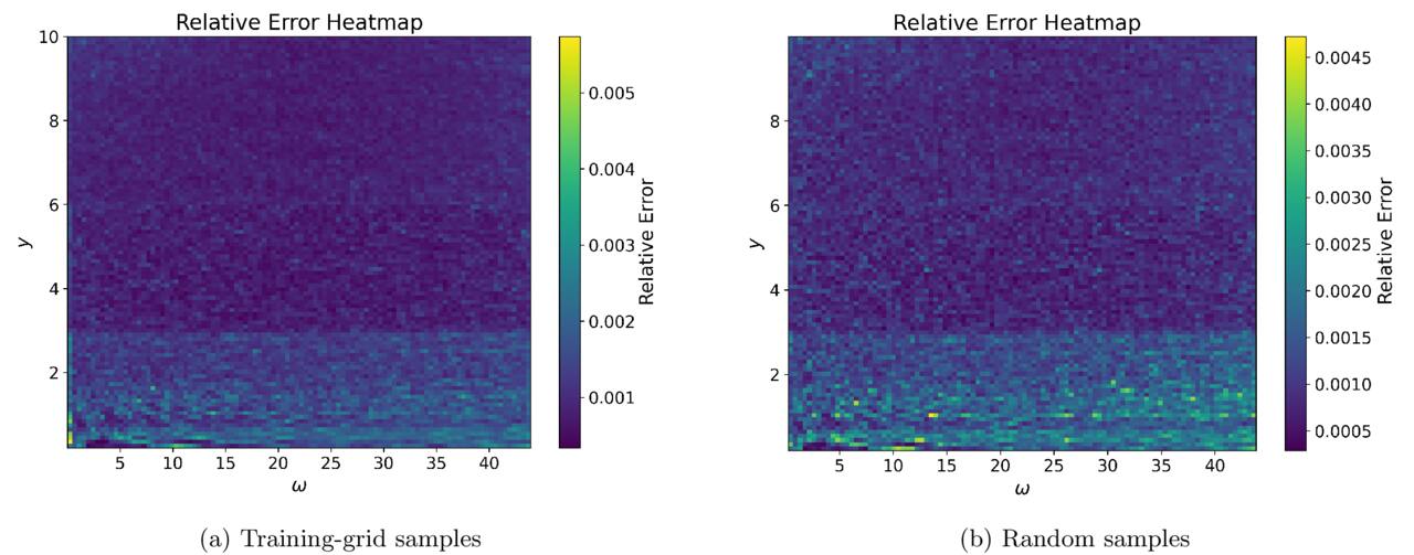
Figure 5. Relative-error heatmaps showing rel as a function of dimensionless frequency ω and source position y.
Download figure:
Standard image High-resolution imageTo provide a comprehensive view of the error behavior across the entire parameter space, particularly near the complex diffraction-interference transition, we visualize the relative-error distribution in Figure 6. The parameter space is represented with a logarithmic axis for the dimensionless frequency ω and a linear axis for the impact parameter y. As illustrated, the model demonstrates remarkable robustness, with the majority of the parameter space generally maintaining relative errors at the  level. Importantly, in the critical transition regime (moderate y ∼ 1 and intermediate ω ∼ 1–10) where the amplification factor exhibits dense and rapid interference fringes, the SIREN architecture maintains high stability without introducing numerical artifacts. We observe a slight elevation in relative errors, occasionally approaching
  , localized strictly in the very-low-frequency regime (ω ∈ [10−2, 10−1]). This minor localized deviation is primarily attributed to the relatively sparse sampling density within this specific subinterval during our training phase. Refining the sampling strategy in this low-frequency regime will be a key direction for our future optimization work.
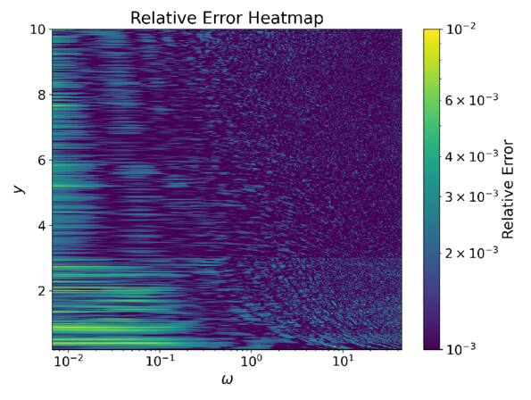
Figure 6. Heatmap of the relative-error distribution across the parameter space. The transition from diffraction to interference (y ∼ 1.0) shows high stability with errors well below the  threshold.
Download figure:
Standard image High-resolution imageFigure 6 illustrates the statistical distribution of these errors. The histogram for off-grid points (Figure 7(a)) is heavily concentrated between 10−8 and 10−3. The cumulative distribution function (CDF) confirms that more than 99% of test points achieve subpercent accuracy. The training-grid statistics (Figure 7(b)) closely mirror the off-grid results, indicating that the model performance on off-grid samples is consistent with the training error.
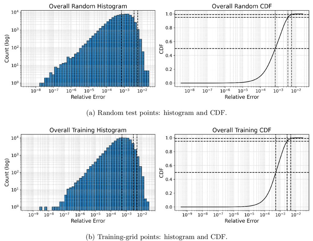
Figure 7. Overall distributions of relative error rel. The nearly identical shape between (a) and (b) indicates excellent generalization.
Download figure:
Standard image High-resolution imageTo verify the physical fidelity of the predictions, Figure 8 presents the waveforms at two representative impact parameters: y = 0.3 (high dynamic range) and y = 1.0 (intermediate regime). At y = 0.3 (Figure 8(a)), the model accurately captures the pronounced central peak (∣F∣ ≈ 2.5) and the subsequent Airy pattern with relative errors consistently below 10−3. At y = 1.0 (Figure 8(b)), the diffraction pattern transitions to a regime with a smoother envelope peak (∣F∣ ≈ 1.4) but increasingly rapid oscillations. The model tracks both the envelope and the phase of the oscillations robustly, maintaining per-mille-level accuracy throughout the spectrum.
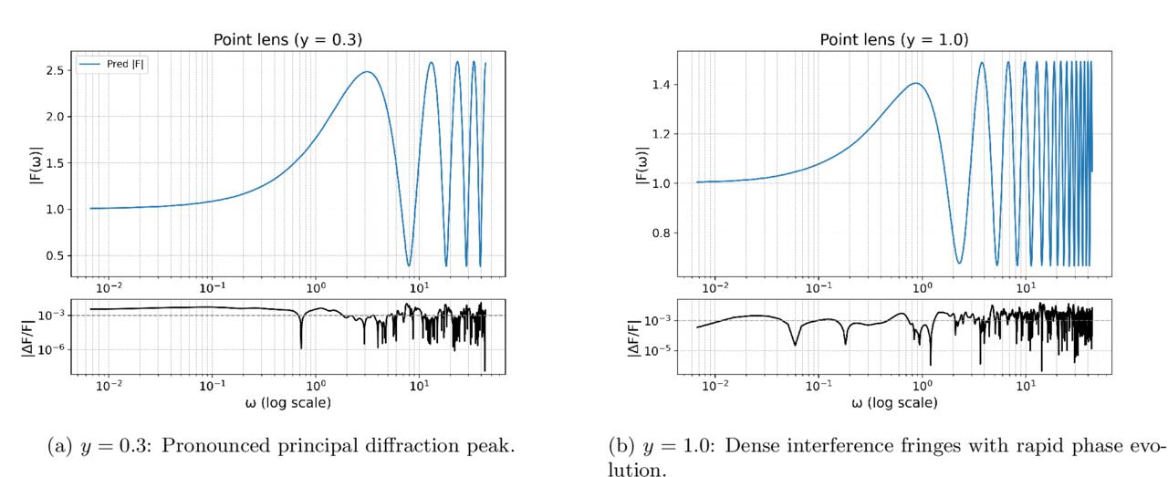
Figure 8. Model prediction versus analytic truth. (a) At y = 0.3, the model captures the high-amplitude peak. (b) At y = 1.0, the model accurately resolves the transitions in oscillation frequency. The bottom panels show the per-frequency relative error, remaining consistently low (∼10−3) in both cases.
Download figure:
Standard image High-resolution image5.2. Spectral Validation
We assess the spectral fidelity of the model using representative impact parameters y = 0.3 and y = 1.0. For a fixed y, we characterize the spectral content of the complex amplification factor by its power spectral density (PSD). We estimate the PSD using the periodogram, defined as the squared modulus of the discrete Fourier transform (DFT; D. B. Percival & A. T. Walden 1993),

where  denotes the DFT applied to the discretized F(ω, y) on a uniform ω-grid, and ν represents the spectral frequency conjugate to ω (quantifying the rate of oscillation of the diffraction fringes). Since we focus on the relative spectral structure, the standard normalization factor is omitted. In practice, the series is mean-subtracted, multiplied by a Tukey window (α = 0.25) to mitigate spectral leakage, and zero-padded to the next power of two prior to the DFT. We verified that the qualitative conclusions are robust to moderate variations in the windowing and padding parameters.
Figure 9 compares the PSDs of the analytic PML solution and the model prediction. At y = 0.3 (Figure 9(a)), the principal diffraction peak and the power-law tail at high ν overlap over several orders of magnitude, indicating that the model preserves both the broadband envelope and the fine-scale oscillatory content. At y = 1.0 (Figure 9(b)), the peak alignment and the asymptotic slope are accurately recovered. While minor residuals appear at intermediate frequencies due to the dense fringe pattern, they do not deviate significantly from the ground-truth scaling. Overall, these tests confirm that the SIREN model successfully reproduces the multiscale spectral structure of F(ω, y) across the relevant domain.
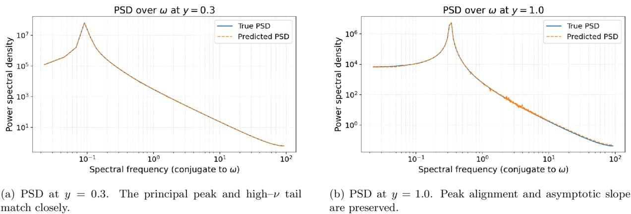
Figure 9. Comparison of power spectral densities (PSDs). The periodograms of the analytic (solid) and model (dashed) amplification factors F(ω, y) are shown on log–log axes. The spectra are computed after demeaning, Tukey windowing (α = 0.25), and zero-padding.
Download figure:
Standard image High-resolution image5.3. Performance Comparison with Numerical Integration Methods
To assess the practical utility of our approach, we compare the SIREN model against the classical ZPAE method (Section 3.1.5), as well as the AE and zero-points integral (ZPI) methods, in terms of both accuracy and computational efficiency. Additionally, we include the high-precision analytical evaluation computed via the mpmath library to serve as our absolute ground-truth baseline.
5.3.1. Accuracy Robustness
We evaluate the accuracy using standard empirical parameters k = 5, ν = 7 (and m = 15 for ZPI) at a fixed frequency ω = 10.0. Figure 10 compares the relative error ∣ΔF∣/∣F∣ as the impact parameter y varies from 0.2 to 5.0.
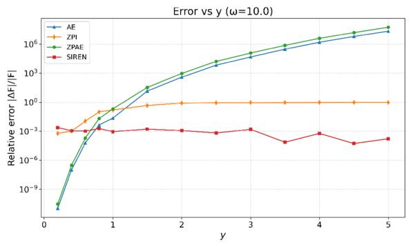
Figure 10. Relative error ∣ΔF/F∣ versus y at fixed ω = 10.0. The ZPAE and AE approximations achieve high accuracy only in the immediate vicinity of the expansion center (y = 0.2) but deteriorate exponentially as y deviates. The ZPI method is stable but yields higher baseline errors. In contrast, the SIREN model maintains stable ∼10−3 accuracy across the entire domain.
Download figure:
Standard image High-resolution imageThe ZPAE and AE methods exhibit extreme sensitivity to the alignment of their expansion centers. While they achieve vanishing residuals (below 10−8) specifically at the anchor point y = 0.2, the approximation error diverges rapidly as y deviates from this configuration. The error increases by orders of magnitude, so the methods require computationally expensive retuning to remain reliable. Meanwhile, the ZPI method, although more stable across the domain, yields a consistently high baseline error under standard truncation settings. In comparison, the SIREN model maintains a uniformly low relative error of order 10−3 across the entire domain. This confirms that the neural network successfully captures the global oscillatory behavior of the diffraction integral without requiring case-by-case hyperparameter adjustments.
5.3.2. Computational Efficiency
To quantify inference latency, we benchmarked the SIREN model against the Mpmath, AE, ZPI, and ZPAE implementations by sampling across representative domains of both ω and y.
As illustrated in Figure 11, the SIREN model achieves a consistent latency of ∼10−5 s per sample. This represents a substantial speedup, being approximately 2 orders of magnitude faster than the high-precision analytic Mpmath baseline (∼10−3 s), up to 4 orders faster than the unoptimized ZPAE and AE implementations (∼10−1 s), and 5 orders faster than the segmented ZPI method (∼100 s).
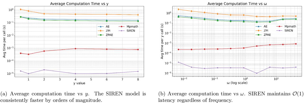
Figure 11. Computational scaling comparison. The plots contrast the analytic integration (Mpmath), AE, ZPI, ZPAE, and the SIREN model. Note that the y-axis is in log scale. The SIREN model demonstrates the lowest latency (∼10−5 s) and exhibits constant-time complexity.
Download figure:
Standard image High-resolution imageFurthermore, the results in Figures 11(a) and (b) demonstrate the robustness of the neural estimator across the parameter space. The computational cost remains stable at this low latency level regardless of variations in the impact parameter y or the frequency ω. This consistent sub-millisecond efficiency is essential for supporting real-time lensing computations and large-scale parameter scans in GW data analysis.
5.4. Phase Accuracy Analysis
We decompose the amplification factor as

and track its phase ϕ. The phase structure is known to affect detectability in matched filtering and to introduce parameter degeneracies. Following the standard definition in circular statistics, we adopt the shortest arc distance as the phase error measure:

Here we additionally report the phase error to highlight the phase fidelity in the wave optics regime.
Table 4 summarizes the mean, median, 95th percentile, and maximum phase errors (in milliradians) for representative impact parameters in each of the four y-intervals. Notably, the maximum phase error observed in our testing is approximately 15.36 mrad. To understand this value, we compare it against the instrumental calibration uncertainty of current GW detectors. During the LIGO O3 observing run, the systematic phase calibration error was estimated to be approximately 2°–5° (∼35–87 mrad) in the sensitive frequency band. Our model’s residual phase error remains well below this instrumental floor. Furthermore, according to waveform accuracy standards, a phase error of this magnitude corresponds to a negligible mismatch, ensuring that the neural network approximation does not introduce significant systematic bias into parameter estimation or reduce the recoverable signal-to-noise ratio (SNR).
Table 4. Phase Error Statistics for Representative y Values in Each Domain Interval (Unit: Mrad)
| Interval | y | Mean | Median | 95th %ile | Maximum |
|---|---|---|---|---|---|

| [0.2, 1.0] | 1.43 | 1.10 | 3.93 | 15.36 |

| [1.0, 3.0] | 1.33 | 1.05 | 3.46 | 9.15 |

| [3.0, 6.0] | 0.26 | 0.22 | 0.61 | 7.56 |

| [6.0, 10.0] | 0.99 | 0.82 | 2.46 | 5.60 |
Download table as: ASCIITypeset image
5.5. Generalization Capability: Extension to SIS Model
To validate the generalization capability of our framework beyond the PML, we extended the pipeline to the SIS model. The primary objective was to verify that the SIREN architecture captures intrinsic wave-optics diffraction behavior rather than overfitting to a specific potential. We employed the identical network architecture and training strategy used for the PML baseline, modifying only the ground-truth generation module to incorporate the SIS diffraction integral (G. Pagano et al. 2020). As shown in Figure 12, the model accurately reconstructs the spectral amplification for representative impact parameters (y = 0.3 and y = 1.0), successfully capturing both the high-amplitude diffraction peaks and the dense interference fringes while maintaining relative errors generally below the 10−3 level. To quantitatively verify this generalization, we evaluated the model on random test points strictly independent of the training grid. The error statistics and distributions are detailed in Appendix B. The SIS model achieves an overall mean relative error of 2.29 × 10⁻⁴, maintaining stable accuracy across the entire evaluated parameter space. This robust performance on out-of-sample data further demonstrates the reliability of the architecture. This successful transferability implies that the proposed neural representation relies on the underlying wave physics rather than specific geometric symmetries, suggesting its broader applicability to more complex lens models.
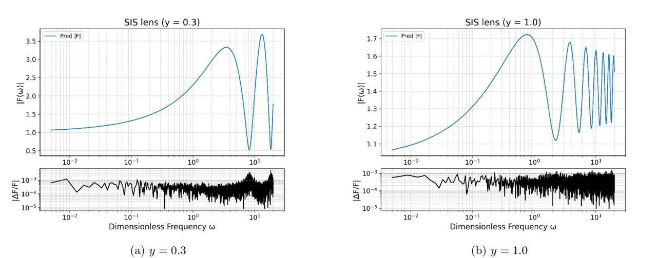
Figure 12. Validation on the SIS model. The SIREN model accurately reconstructs the spectral amplification ∣F(ω)∣ (top panels) and maintains low relative errors (bottom panels) for both strong-lensing (y = 0.3) and transition (y = 1.0) regimes, demonstrating the method’s transferability.
Download figure:
Standard image High-resolution image5.6. Generalization Capability: Extension to SIS Model
To validate the generalization capability of our framework beyond the PML, we extended the pipeline to the SIS model. The primary objective was to verify that the SIREN architecture captures intrinsic wave-optics diffraction behavior rather than overfitting to a specific potential. We employed the identical network architecture and training strategy used for the PML baseline, modifying only the ground-truth generation module to incorporate the SIS diffraction integral (G. Pagano et al. 2020). As shown in Figure 12, the model accurately reconstructs the spectral amplification for representative impact parameters (y = 0.3 and y = 1.0). To quantitatively verify this generalization, we evaluated the model on random test points strictly independent of the training grid. The error statistics and distributions are detailed in Appendix B. The SIS model achieves an overall mean relative error of 2.29 × 10⁻⁴, maintaining stable accuracy across the entire evaluated parameter space. This robust performance on out-of-sample data further demonstrates the reliability of the architecture. This successful transferability implies that the proposed neural representation relies on the underlying wave physics rather than specific geometric symmetries, suggesting its broader applicability to more complex lens models.
6. Conclusions
This study establishes a neural representation framework based on SIRENs to resolve computational bottlenecks in wave-optics lensing. The network’s periodic activation functions naturally match the diffraction integral’s oscillatory kernel, enabling the model to capture high-frequency spectral features. Quantitatively, the method achieves a relative accuracy of  and speeds up computation by ∼100× compared to numerical integration. Concurrently, the framework shifts the heavy computational burden from “online integration” to “offline training,” resulting in
  inference complexity that remains constant regardless of the oscillation frequency. This constant-time inference performance offers a potential solution to the computational bottleneck in Bayesian parameter estimation pipelines. By providing fast and accurate likelihood evaluations with a stable execution time that remains independent of parameter variations, our framework supports a practical pathway toward tractable wave-optics parameter estimation for future GW data analysis.
A key feature of the model is its dimensionless formulation, which ensures intrinsic scale invariance. While we validated the framework using stellar-mass lenses typical of LVK observations, this design allows direct application to supermassive black hole lensing in the LISA band without retraining. High efficiency is essential for third-generation detectors, such as the Einstein Telescope (ET; M. Maggiore et al. 2020) and Cosmic Explorer (CE; D. Reitze et al. 2019). These instruments will likely detect hundreds of high-SNR lensing events annually (X. Ding et al. 2015; L. Yang et al. 2022; Z. Gao et al. 2023). Such a data volume is too high for traditional online integration methods, making our approach a necessary alternative.
In summary, coordinate-based neural representations provide a robust tool for precision astronomy. Beyond gravitational lensing, matching neural architectures to physical kernels offers an effective path to accelerate the analysis of highly oscillatory systems in broader physical contexts.
Acknowledgments
F.Z. would like to thank the MIT LIGO Laboratory for its continuous support and advice. F.Z. is supported by the National Natural Science Foundation of China (grant No. 62372409) and Ministry of Science and Technology of the People’s Republic of China (grant No. 2023ZD0120704 of project No. 2023ZD0120700).
Appendix A: Per-interval Error Distributions
This Appendix provides detailed histograms and CDFs for each of the four impact parameter intervals discussed in the main text.
The per-interval histograms and CDFs in Figures 13(a) and (b) (I1, y ∈ [0.2, 1.0]) show that off-grid errors are concentrated toward the higher end of our overall range, with a visible upper tail. The training-grid distribution closely matches the off-grid case and shows a slightly lower center, indicating comparable accuracy and stable generalization in the near-alignment band.
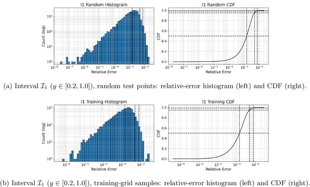
Figure 13. Error distributions in the smallest y-interval. Panel (a) shows the distribution over 20,000 random (ω, y) samples, while panel (b) shows the same statistics on the original training grid. Histograms (left halves) use log-scaled counts and bins; CDFs (right halves) mark the 1%, 5%, 10%, and 90% quantiles.
Download figure:
Standard image High-resolution imageFigures 14(a) and (b) (I2, y ∈ [1.0, 3.0]) display a clear leftward shift relative to I1. Most probability mass moves toward smaller errors while the CDF rises more steeply, and the training-grid curves remain well aligned with the off-grid curves. This behavior reflects improved accuracy as y moves away from near alignment.
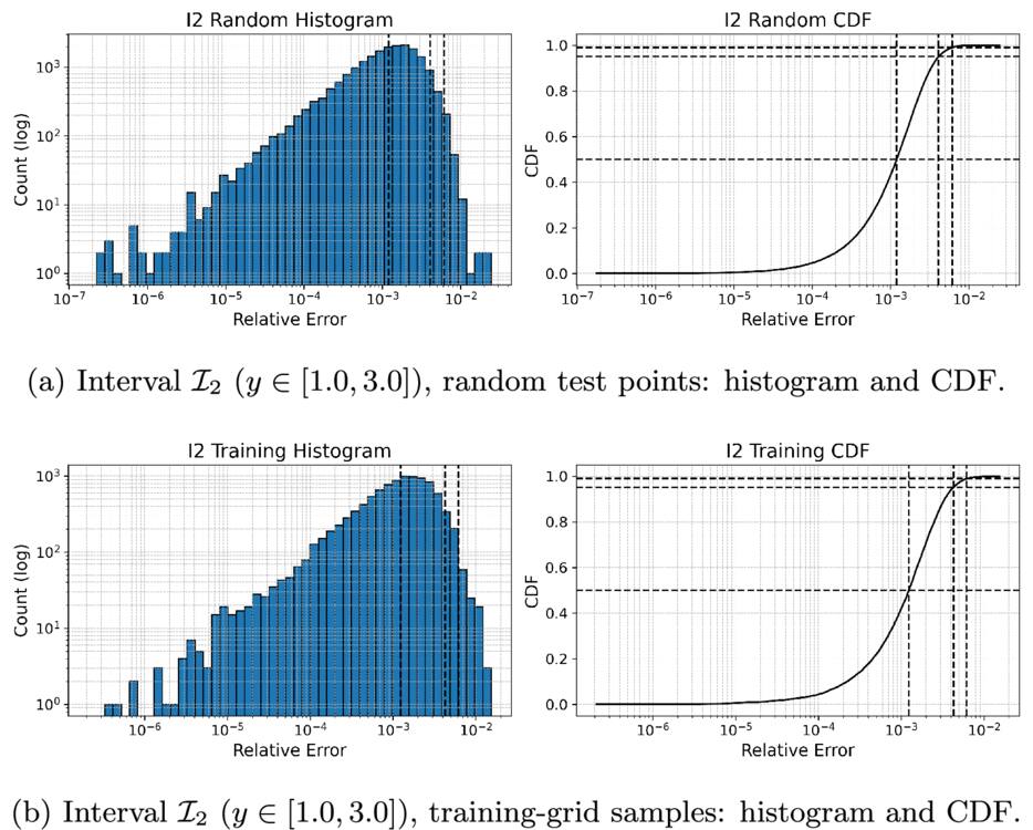
Figure 14. Error distributions in the low-to-moderate y-interval. Random-point (a) and grid-point (b) errors both concentrate in the 10−7–10−3 range, with more than 90% of samples below 10−4 error.
Download figure:
Standard image High-resolution imageFigures 15(a) and (b) (I3, y ∈ [3.0, 6.0]) present the tightest distributions among all intervals. The histogram peak lies at the low-error end and the CDF shows a rapid rise, with very weak upper tails. Off-grid and training-grid results are nearly indistinguishable, indicating the highest accuracy and the strongest tail suppression in this intermediate band.
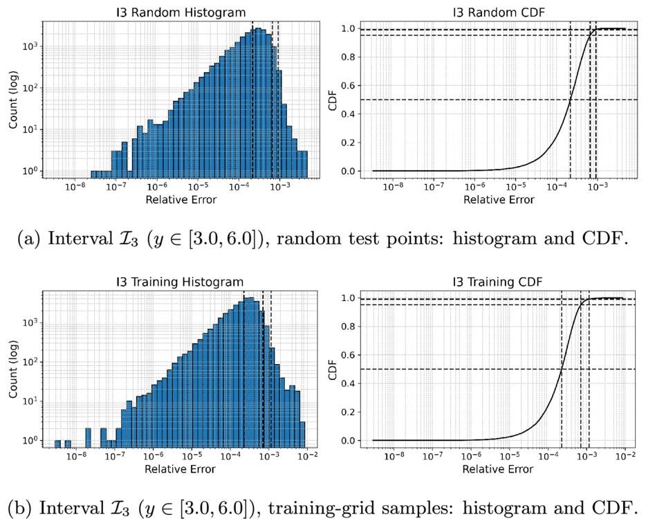
Figure 15. Error distributions in the moderate y-interval. Both random and grid CDFs (panels (a) and (b)) exceed 97% below 10−5 error, indicating peak network accuracy in this middle interval.
Download figure:
Standard image High-resolution imageFigures 16(a) and (b) (I4, y ∈ [6.0, 10.0]) remain close to I3 in both scale and shape. Off-grid and training-grid distributions again agree well. A mild elevation is visible only in a small portion of the domain associated with large y and high ω, while the bulk of the mass remains at per-mille-level errors.
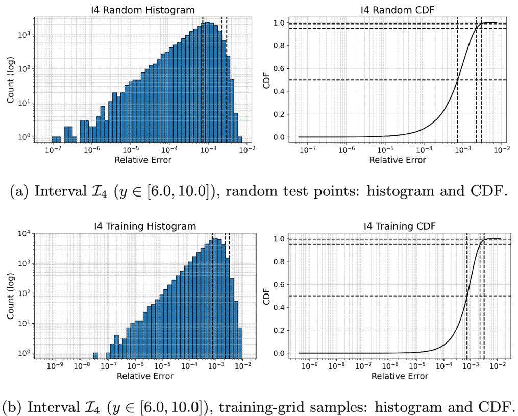
Figure 16. Error distributions in the largest y-interval. Even in this high-frequency interval, over 95% of points in both random (a) and grid (b) cases remain below 10−4 error.
Download figure:
Standard image High-resolution imageAcross all intervals the off-grid statistics mirror the training-grid statistics, and the ordering I1 > I2 > I3 ≈ I4 is consistent with the summary in Table 3. Errors are relatively higher for small y, reach their lowest levels for 3 ≤ y ≤ 6, and increase slightly only near the high-y, high-ω corner. Overall, the model maintains per-mille-level accuracy with fast upper-tail decay and consistent generalization beyond the training points. For quantitative summaries, including mean, median, and upper-tail percentiles, see Table 3.
Appendix B: SIS Model Error Distributions
We provide detailed quantitative metrics for the SIS model evaluation to demonstrate the robustness of our architecture across different physical regimes. The model was tested on random off-grid points across four intervals of the impact parameter y. Table 5 summarizes the complex relative-error performance. The overall mean relative error is 2.29 × 10⁻⁴, confirming the high accuracy of the SIREN architecture on the SIS potential.
Table 5. Summary of the SIS Model Relative-error Performance
| Metric | Overall |

|

|

|
![${{ \mathcal I }}_{4}[6.0,10.0]$](https://content.cld.iop.org/journals/0067-0049/284/2/48/revision1/apjsae64e4ieqn67.gif)
|
|---|---|---|---|---|---|
| Mean rel. error | 2.29 × 10⁻⁴ | 1.25 × 10⁻³ | 1.00 × 10⁻⁴ | 6.51 × 10⁻⁵ | 1.60 × 10⁻⁴ |
| Median rel. error | 8.83 × 10⁻⁵ | 3.83 × 10⁻⁴ | 6.94 × 10⁻⁵ | 4.97 × 10⁻⁵ | 1.26 × 10⁻⁴ |
| 95th percentile | 4.91 × 10⁻⁴ | 3.58 × 10⁻³ | 2.22 × 10⁻⁴ | 1.83 × 10⁻⁴ | 4.10 × 10⁻⁴ |
| 99th percentile | 1.30 × 10⁻³ | 8.08 × 10⁻³ | 7.24 × 10⁻⁴ | 2.46 × 10⁻⁴ | 6.01 × 10⁻⁴ |
| Maximum error | 1.97 × 10⁻² | 1.97 × 10⁻² | 7.20 × 10⁻³ | 5.91 × 10⁻³ | 4.07 × 10⁻³ |
Note. Metrics include mean, median, 95th/99th percentiles, and maximum error evaluated on random test samples.
Download table as: ASCIITypeset image
Consistent with the PML baseline, the performance breakdown reveals that the most challenging region is the innermost interval  . Here the amplification factor exhibits sharp amplitude gradients and high dynamic range due to strong lensing and caustic proximity, resulting in a slightly elevated mean error of 1.25 × 10⁻³. Conversely, for moderate-to-large impact parameters (
 to
to  ), where dense wave-optics interference fringes dominate, the SIREN architecture perfectly resolves the rapid phase oscillations, suppressing the mean relative errors to the 10−5 and 10−4 levels.
Figure 17 further visualizes this stability by illustrating the statistical distribution of the overall relative errors. The histogram (left panel) is heavily concentrated around 10−4 with a rapid decay in the upper tail. The CDF (right panel) explicitly confirms that 95% of the unseen test points achieve an error below 4.91 × 10⁻⁴, and 99% are strictly bounded below 1.30 × 10⁻³. The absence of catastrophic outliers in this distribution matches the strong generalization behavior observed in the PML baseline, verifying that the neural framework reliably captures the underlying diffraction integral rather than overfitting.
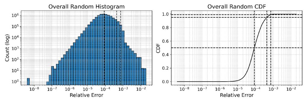
Figure 17. Overall distributions of relative error for the SIS model on random test points. The histogram (left) and CDF (right) demonstrate stable generalization and bounded extreme errors.
Download figure:
Standard image High-resolution image