Abstract
The determination of exoplanet properties and occurrence rates using Kepler data critically depends on our knowledge of the fundamental properties (such as temperature, radius, and mass) of the observed stars. We present revised stellar properties for 197,096 Kepler targets observed between Quarters 1–17 (Q1-17), which were used for the final transiting planet search run by the Kepler Mission (Data Release 25, DR25). Similar to the Q1–16 catalog by Huber et al., the classifications are based on conditioning published atmospheric parameters on a grid of Dartmouth isochrones, with significant improvements in the adopted method and over 29,000 new sources for temperatures, surface gravities, or metallicities. In addition to fundamental stellar properties, the new catalog also includes distances and extinctions, and we provide posterior samples for each stellar parameter of each star. Typical uncertainties are ∼27% in radius, ∼17% in mass, and ∼51% in density, which is somewhat smaller than previous catalogs because of the larger number of improved  constraints and the inclusion of isochrone weighting when deriving stellar posterior distributions. On average, the catalog includes a significantly larger number of evolved solar-type stars, with an increase of 43.5% in the number of subgiants. We discuss the overall changes of radii and masses of Kepler targets as a function of spectral type, with a particular focus on exoplanet host stars.
1. Introduction
Since the launch of the NASA Kepler mission (Borucki et al. 2010; Koch et al. 2010) in 2009, a tremendous number of discoveries in exoplanet science have been made possible thanks to the near-continuous high-precision photometric data collected for over four years. To date, 4706 planet candidates have been identified, over 49% of which have been confirmed or validated (Rowe et al. 2014; Morton et al. 2016). This large number of detections allowed statistical studies of planet occurrence rates (e.g., Howard et al. 2012; Fressin et al. 2013; Burke et al. 2015; Dressing & Charbonneau 2015; Silburt et al. 2015) as well as numerous individual discoveries such as Kepler’s first rocky exoplanet, Kepler-10b (Batalha et al. 2011), circumbinary planets (e.g., Orosz et al. 2012b; Kostov et al. 2014; Welsh et al. 2015), or the detection of planets in or near the habitable zone (e.g., Ballard et al. 2013; Barclay et al. 2013; Borucki et al. 2013; Torres et al. 2015; Kane et al. 2016).
Stellar astrophysics also benefited from the exquisite data of Kepler with a large number of breakthrough discoveries, such as the asteroseismic measurement of the internal rotation (Beck et al. 2012; Deheuvels et al. 2012, 2014; Mosser et al. 2012) and magnetic fields (Fuller et al. 2015; Stello et al. 2016) of subgiants and red giants, the detection of surface rotation and its relation to ages of solar-like stars (e.g., García et al. 2014; McQuillan et al. 2014; Ceillier et al. 2016; van Saders et al. 2016), and the measurement of magnetic activity of main-sequence stars (e.g., Mathur et al. 2014; Arkhypov et al. 2015; Salabert et al. 2016). Asteroseismic data of red giants are now also used to perform galactic archeology by combining them with high-resolution spectroscopy (e.g., Pinsonneault et al. 2014; Rodrigues et al. 2014; Martig et al. 2015).
Since the transit technique measures planet properties only relative to the host star, it is crucial to characterize the parameters of the host stars to derive precise parameters of the planets. Before the launch of the mission, the Kepler Input Catalog (KIC Brown et al. 2011) was constructed based on broadband photometry, with the primary purpose to select targets for observations (Batalha et al. 2010) and provide an initial classification of planet candidates. In order to improve the KIC, Huber et al. (2014) presented revised stellar properties for 196,468 Kepler targets, which were used for the Q1–16 Transit Planet Search and Data Validation run (Tenenbaum et al. 2014). The catalog was based on atmospheric properties (temperature  , surface gravity
  , and metallicity [Fe/H]) published in the literature using a variety of methods (asteroseismology, spectroscopy, exoplanet transits, and photometry), which were then homogeneously fitted to a grid of Dartmouth (DSEP) isochrones (Dotter et al. 2008). The catalog was updated in early 2015 for a Q1-17 transit detection run (Data Release 2416
, DR24, Huber 2014) based on the latest classifications of Kepler targets in the literature and using the same method as Huber et al. (2014). We discarded the stars observed only in Q0 as the transit search pipeline does not investigate the data from the commissioning phase for planets. However, we note that 180 stars with only Q0 data have slipped into the catalog during the input data consolidation.
, and metallicity [Fe/H]) published in the literature using a variety of methods (asteroseismology, spectroscopy, exoplanet transits, and photometry), which were then homogeneously fitted to a grid of Dartmouth (DSEP) isochrones (Dotter et al. 2008). The catalog was updated in early 2015 for a Q1-17 transit detection run (Data Release 2416
, DR24, Huber 2014) based on the latest classifications of Kepler targets in the literature and using the same method as Huber et al. (2014). We discarded the stars observed only in Q0 as the transit search pipeline does not investigate the data from the commissioning phase for planets. However, we note that 180 stars with only Q0 data have slipped into the catalog during the input data consolidation.
In this work we present another major update of the Kepler stellar properties catalog for 197,096 Kepler targets. The catalog was developed to support the final transit detection run (Data Release 25, hereafter DR25) before the close-out of the Kepler mission. Initial plans for the catalog included a homogeneous reclassification based on broadband colors alone (i.e., without relying on classifications from the KIC, see Section 9 in H14). However, the limited sensitivity of available broadband colors and the complexity of constructing priors that accurately reproduce the Kepler target selection function made such a classification scheme unfeasible for the delivery of the catalog. Similar to previous versions, the updated catalog presented here is therefore based on the consolidation of atmospheric properties (temperature  , surface gravity
  , and metallicity
 ![$[\mathrm{Fe}/{\rm{H}}]$](https://content.cld.iop.org/journals/0067-0049/229/2/30/revision1/apjsaa567bieqn6.gif) ) that were either published in the literature or provided by the Kepler community follow-up program (CFOP, Gautier et al. 2010), with input values taken from different methods such as asteroseismology, spectroscopy, Flicker, and photometry.
) that were either published in the literature or provided by the Kepler community follow-up program (CFOP, Gautier et al. 2010), with input values taken from different methods such as asteroseismology, spectroscopy, Flicker, and photometry.
2. Consolidation of Input Values
2.1. Inputs in Previous Catalogs
The stellar properties in the KIC were derived from Sloan griz and 2MASS JHK broadband photometry as well as an intermediate-band filter D51 that has some sensitivity to surface gravity. More details on the method used to build the KIC can be found in Brown et al. (2011). Several studies have showed a few shortcomings with the KIC. For instance, Pinsonneault et al. (2012) used KIC griz photometry for more than 120,000 dwarfs to derive temperatures from color-temperature relations, and found that the KIC effective temperatures are underestimated by up to 200 K. Moreover, several studies have shown that the KIC surface gravities appear to be overestimated for solar-type stars, based on comparisons to asteroseismology (Verner et al. 2011), spectroscopy (Everett et al. 2013), and surface gravities derived from stellar granulation (Bastien et al. 2014).
In the Q1–16 catalog, H14 consolidated literature values for temperature, surface gravity, and metallicity from asteroseismology, transits, spectroscopy, photometry, and the KIC to derive the fundamental properties of Kepler targets by fitting isochrones to these observables. However, several shortcomings remained in that catalog. For instance, 70% of all Kepler target  and [Fe/H] values were still based on the KIC, a number of targets without KIC stellar parameters remained unclassified, and the method that was adopted to infer stellar properties did not use priors for inferring posterior distributions. The motivation for this updated catalog was to overcome some of these shortcomings, in particular to assemble the most homogeneous catalog possible with the most recent observables available for all Kepler targets.
2.2. New Input Values
The main new input values for the DR25 stellar properties catalog can be summarized as follows:
- 1.For 6383 stars we used the effective temperatures available from Data Release 1 (Luo et al. 2015) of the Large Sky Area Multi-Object Fiber Spectroscopic Telescope (LAMOST, Xinglong observatory, China) survey (Zhao et al. 2012). The classifications are based on medium-resolution (R ∼ 1800) spectra and cover a large number of stars in the Kepler field. There is a specific project between LAMOST and the Kepler field (De Cat et al. 2015), but the delivery of the stellar parameters (Frasca et al. 2016) was provided outside the timeframe of our catalog. The comparison of the DR25 and the LAMOST-Kepler spectroscopic results showed a good agreement in general with a standard deviation of the temperature differences of 228 K for dwarfs and 205 K for red giants and of surface gravity of 0.26 dex for dwarfs and 0.40 dex for red giants.
- 2.The Apache Point Observatory for Galactic Evolution Experiment (APOGEE, Majewski et al. 2015) also targeted a large number of Kepler stars to obtain high-resolution (R ∼ 22,500) H-band spectra, mostly for red giant stars. We adopted the effective temperature from APOGEE for 5678 stars, surface gravities for 1544 stars, and metallicities for 5662 stars from DR12 (Alam et al. 2015).
- 3.For 14,535 stars we adopted surface gravities estimated from the detection of granulation in the Kepler light curves (the Flicker method, Bastien et al. 2016). We limited the Flicker
 values to stars for which the reported uncertainty was smaller than 0.2 dex to ensure a higher reliability of the input values.
 - 4.For more than 1000 stars, we used spectroscopic parameters (, , ) provided by the Kepler CFOP that observed around 800 planet candidate host stars and 535 solar-like stars for which solar-like oscillations had been detected in the Kepler data.
- 5.We included a sample of 835 stars that were classified as dwarfs in the original KIC, but were shown to be red giants based on the detection of giant-like oscillations in the Kepler data. We adopted values estimated from asteroseismology in combination with revised effective temperatures for these stars (Mathur et al. 2016).
- 6.For 62 newly confirmed Kepler exoplanet hosts we adopted stellar parameters (, , ) as published in the discovery papers.
- 7.We also report spectroscopic parameters (, , ) for 317 stars that were unclassified so far, but were included in either the APOGEE or LAMOST surveys.
- 8.We added 311 stars that were new targets observed during Q17.


![$[\mathrm{Fe}/{\rm{H}}]$](https://content.cld.iop.org/journals/0067-0049/229/2/30/revision1/apjsaa567bieqn11.gif)


![$[\mathrm{Fe}/{\rm{H}}]$](https://content.cld.iop.org/journals/0067-0049/229/2/30/revision1/apjsaa567bieqn15.gif)


![$[\mathrm{Fe}/{\rm{H}}]$](https://content.cld.iop.org/journals/0067-0049/229/2/30/revision1/apjsaa567bieqn18.gif)
Compared to the H14 catalog, new input values are used for 14.7% of the stars. In this final catalog, the input  values are taken from seismology for 16,947 stars (8.6% of the stars), from Flicker for 14,535 stars (7.4%), from spectroscopy for 9277 stars (4.7%) and from the KIC for 143,785 stars, corresponding to ∼72.9% of the total sample compared to ∼84% for the H14 catalog. The remaining stars have their
  input values either from photometry or transit search. For the input effective temperature, the source is spectroscopy for 14,813 stars, non-KIC photometry for 151,118 stars, and the KIC for 31,165 stars.
Figure 1 shows an HR diagram of the largest sources of new input values, namely LAMOST, APOGEE, Flicker, CFOP, and the sample of misclassified red giants. Figure 2 represents the stars that were added compared to the H14 catalog, which are either stars that remained unclassified in the Q1–16 as a result of a lack of 2MASS photometry or targets that were first observed in Q17. There is no overlap between the new Q17 targets and the unclassified stars with LAMOST and APOGEE spectra. Of the new 628 additional stars, 294 are red giants and 332 are dwarfs, the remaining stars are subgiants.
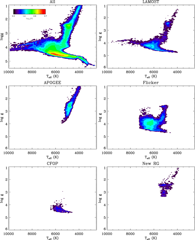
Figure 1. Input surface gravity and effective temperature for the full catalog (top left panel) and for the five largest sources of new input values (see legend on the top of each panel). Color-coding denotes the logarithmic number density as shown in the color bar in the top left panel.
Download figure:
Standard image High-resolution image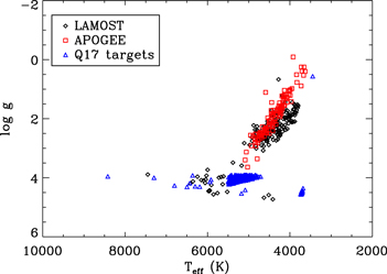
Figure 2. Surface gravity vs. effective temperature for targets that were newly added compared to the Q1–16 catalog. Different symbols show stars with classifications adopted from LAMOST (black diamonds), APOGEE (red squares), and new stars targeted during Q17 (blue triangles).
Download figure:
Standard image High-resolution imageGiven that some stars have input parameters from different literature sources, a prioritization scheme had to be adopted. This prioritization was mostly based on the precision and accuracy of the sources used to derive the input values, as follows. For surface gravity, the highest priority was given to asteroseismology, then high-resolution (HR) spectroscopy, low-resolution (LR) spectroscopy, Flicker, photometric observations, and finally the KIC. For the temperature and metallicity, the highest priority was given to high-resolution spectroscopy, low-resolution spectroscopy, photometric observations, and the KIC. In other words, priority was given to the CFOP observations and published values for confirmed planets, then APOGEE, LAMOST, and finally to the KIC. The prioritization scheme is given in Table 1.
Table 1. Priority List for Input Surface Gravity, Effective Temperature, and Metallicity from Different Techniques
| Parameter | Priority | Input |
|---|---|---|

|
1 | Asteroseismology |
| 2 | HR spectroscopy | |
| 3 | LR spectroscopy | |
| 4 | Flicker | |
| 5 | KIC | |
 /[Fe/H] /[Fe/H] |
1 | HR spectroscopy |
| 2 | LR spectroscopy | |
| 3 | Photometry | |
| 4 | KIC | |
Note. LR—low resolution (R ≤ 5000); HR—high resolution (R ≥ 5000).
Download table as: ASCIITypeset image
Typical uncertainties associated with each observable are taken from H14 and listed in Table 2. In addition, we adopted a typical uncertainty of 0.2 dex for the Flicker  g. These are the uncertainties used as inputs.
Table 2. Uncertainties Adopted for the Input Parameters
| Method |

|

|
![${\sigma }_{[\mathrm{Fe}/{\rm{H}}]}$](https://content.cld.iop.org/journals/0067-0049/229/2/30/revision1/apjsaa567bieqn26.gif)
|
|---|---|---|---|
| (%) | (dex) | (dex) | |
| Asteroseismology | ⋯ | 0.03 | ⋯ |
| Transits | ⋯ | 0.05 | ⋯ |
| Spectroscopy | 2 | 0.15 | 0.15 |
| Flicker | ⋯ | 0.20 | ⋯ |
| Photometry | 3.5 | 0.40 | 0.30 |
| KIC | 3.5 | 0.40 | 0.30 |
Download table as: ASCIITypeset image
The input values and provenances used for the full catalog are listed in Table 3. Following H14, the provenances are comprised of three letters and a number corresponding to the reference key of Table 5 in Appendix
Table 3. Input Values of the DR25 Stellar Properties Catalog
| KIC |

|

|
[Fe/H] |

|

|

|
|---|---|---|---|---|---|---|
| 757076 | 5164 ± 154 | 3.601 ± 0.400 | −0.083 ± 0.300 | PHO1 | KIC0 | KIC0 |
| 757099 | 5521 ± 168 | 3.817 ± 0.400 | −0.208 ± 0.300 | PHO1 | KIC0 | KIC0 |
| 757137 | 4751 ± 139 | 2.378 ± 0.030 | −0.079 ± 0.300 | PHO1 | AST9 | KIC0 |
| 757280 | 6543 ± 188 | 4.082 ± 0.400 | −0.231 ± 0.300 | PHO1 | KIC0 | KIC0 |
| 757450 | 5330 ± 106 | 4.500 ± 0.050 | −0.070 ± 0.150 | SPE51 | TRA51 | SPE51 |
| 891901 | 6325 ± 186 | 4.411 ± 0.400 | −0.084 ± 0.300 | PHO1 | KIC0 | KIC0 |
| 891916 | 5602 ± 165 | 4.591 ± 0.400 | −0.580 ± 0.300 | PHO1 | KIC0 | KIC0 |
| 892010 | 4834 ± 151 | 2.163 ± 0.030 | 0.207 ± 0.300 | PHO1 | AST9 | KIC0 |
| 892107 | 5086 ± 161 | 3.355 ± 0.400 | −0.085 ± 0.300 | PHO1 | KIC0 | KIC0 |
| 892195 | 5521 ± 184 | 3.972 ± 0.400 | −0.054 ± 0.300 | PHO1 | KIC0 | KIC0 |
| 892203 | 5945 ± 208 | 4.081 ± 0.400 | −0.118 ± 0.300 | PHO1 | KIC0 | KIC0 |
| 892376 | 3963 ± 138 | 4.471 ± 0.400 | 0.122 ± 0.300 | KIC0 | KIC0 | KIC0 |
| 892667 | 6604 ± 209 | 4.100 ± 0.400 | −0.256 ± 0.300 | PHO1 | KIC0 | KIC0 |
| 892675 | 6312 ± 208 | 4.048 ± 0.400 | −0.257 ± 0.300 | PHO1 | KIC0 | KIC0 |
| 892678 | 6136 ± 177 | 3.939 ± 0.400 | −0.260 ± 0.300 | PHO1 | KIC0 | KIC0 |
Note. See Table 5 for the reference key for the provenances listed in the last three columns.
Only a portion of this table is shown here to demonstrate its form and content. A machine-readable version of the full table is available.
Download table as: DataTypeset image
3. Catalog Construction
3.1. Method
We followed H14 by comparing the input  ,
,  and
and ![$[\mathrm{Fe}/{\rm{H}}]$](https://content.cld.iop.org/journals/0067-0049/229/2/30/revision1/apjsaa567bieqn34.gif) values to stellar evolution models in order to infer additional stellar parameters such as radii, which are required by the Kepler planet detection pipeline. For the current catalog we adopted the isochrones from the Dartmouth Stellar evolution Database (DSEP, Dotter et al. 2008), which cover a wide range in parameter space and have demonstrated good agreement with interferometric observations of low-mass dwarfs. We improved the original DSEP grid adopted by H14 by interpolating each isochrone of a given age and [Fe/H] in mass to yield a step size of at most 0.02 M☉ for all models with
values to stellar evolution models in order to infer additional stellar parameters such as radii, which are required by the Kepler planet detection pipeline. For the current catalog we adopted the isochrones from the Dartmouth Stellar evolution Database (DSEP, Dotter et al. 2008), which cover a wide range in parameter space and have demonstrated good agreement with interferometric observations of low-mass dwarfs. We improved the original DSEP grid adopted by H14 by interpolating each isochrone of a given age and [Fe/H] in mass to yield a step size of at most 0.02 M☉ for all models with  , which removes significant gaps in the original grid for cool dwarfs. The final grid included around
  models and spanned from 1 to 15 Gyr in steps of 0.5 Gyr in age and −2.5–0.56 dex in steps of 0.02 dex in
 ![$[\mathrm{Fe}/{\rm{H}}]$](https://content.cld.iop.org/journals/0067-0049/229/2/30/revision1/apjsaa567bieqn37.gif) .
.
We followed the method described by Serenelli et al. (2013) to infer stellar parameters from isochrones. Given a set of input values ![$x=\{{T}_{\mathrm{eff}},\mathrm{log}g,[\mathrm{Fe}/{\rm{H}}]\}$](https://content.cld.iop.org/journals/0067-0049/229/2/30/revision1/apjsaa567bieqn38.gif) with Gaussian uncertainties
with Gaussian uncertainties  and a set of intrinsic parameters
 ![$y=\{\mathrm{age},\ [\mathrm{Fe}/{\rm{H}}],\ \mathrm{mass}\}$](https://content.cld.iop.org/journals/0067-0049/229/2/30/revision1/apjsaa567bieqn40.gif) , we calculated the posterior probability of the observed star having intrinsic parameters y as
, we calculated the posterior probability of the observed star having intrinsic parameters y as

We adopted flat priors p(y) for mass, age, and metallicity. Probability distribution functions for any given stellar parameter were then obtained by weighting  by the volume that each isochrone point encompasses in mass, age, and metallicity, and summing the resulting distribution along a given stellar parameter. The bin size was initially fixed to either an absolute value for
  , [Fe/H], mass, and density, or to a fractional step size of the best-fit value for radius and distance. From this initial distribution we calculated the 1σ confidence interval, and then iterated the step size to yield at least 10 bins within a 1σ confidence interval. The posteriors calculated using this method are hereafter referred to as “discrete posteriors.”
Figure 3 shows examples of discrete posteriors in effective temperature and surface gravity for three stars with an input  from the KIC (top left panel), spectroscopy (top middle panel), and asteroseismology (top right panel) and an input
  from the KIC (bottom left panel) and spectroscopy (bottom middle and bottom right panels). The large input uncertainty in
  for the KIC yields a distribution that peaks near the main sequence (the most probable for a star with a weak
  constraint) and has a tail toward lower
  values, reflecting the uncertainty of the evolutionary state of the star. On the other hand, the smaller uncertainty of the spectroscopic and asteroseismic
  and spectroscopic
  values yields discrete posteriors that are considerably more narrow.
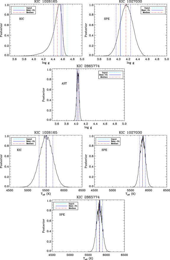
Figure 3. Discrete posterior distributions for surface gravity (top panels) and effective temperature (bottom panels) for three different stars. Input values in  were adopted from KIC (left panel), spectroscopy (middle panel), and asteroseismology (right panels). Input values in
  were adopted from KIC (left panel) and spectroscopy (middle and right panel). The dashed cyan line marks the input value and the solid blue line is the output value with associated uncertainties (blue dashed lines). The dash–dotted red line corresponds to the median value of the distribution.
Download figure:
Standard image High-resolution imageSince the Kepler pipeline requires a single value and uncertainty for each stellar parameter, a suitable summary statistic had to be chosen. We decided to report the best-fit value (calculated by maximizing Equation (1)), with an uncertainty derived from the 1σ interval around the best fit. As shown in Figure 3, the best-fit value does not always coincide with the mode of the posterior distribution. Adopting the best fit was motivated by the fact that adopting the mode or median as a point estimate would lead to an unrealistically high number of main-sequence stars because for a given input value of  with a large uncertainty, a star will probabilistically be most likely on the main sequence. Since the Kepler target stars represent neither a volume nor a strictly magnitude-limited sample (see, for example, the target selection criteria as described in Batalha et al. 2010), constructing a prior to characterize the most probable evolutionary state of a Kepler target star is not straightforward. The stellar classification in the KIC used a prior constructed from a volume-limited Hipparcos sample, which has been shown to underestimate the number of subgiants due to Malmquist bias (see for example Bastien et al. 2014). Adopting the best-fit values ensures that the point estimates reported in the catalog account for some of the expected Malmquist bias in the Kepler sample, but we caution that some systematic biases likely remain in the catalog.
3.2. Stellar Parameter Uncertainties
Uncertainties for each reported stellar parameter are calculated from the 1σ interval around the best fit (Figure 3). Figure 4 shows the distribution of fractional uncertainties over all targets for various stellar parameters. We note that surface gravity and radius show a bimodal distribution, which is due to the two main provenances of the surface gravity input values from seismology and from the KIC with associated uncertainties of 0.03 dex and 0.40 dex, respectively. We observe a similar bimodality with peaks at ∼80 and ∼150 K for effective temperatures based on spectroscopic and photometric input values. While the bimodality in radius and gravity was also present in the H14 catalog, the bimodality in  is new and reflects the increase in the number of stars that now have spectroscopic observations.
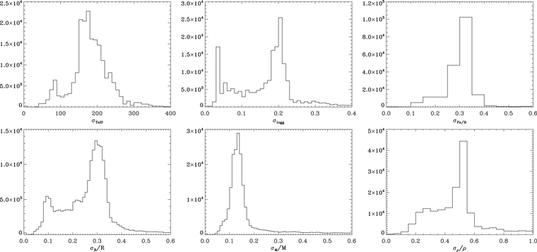
Figure 4. Distribution of absolute uncertainties in  ,
,  , and [Fe/H] and relative uncertainties in radius, mass, and density for all stars in the sample.
Download figure:
Standard image High-resolution imageThe typical reported uncertainties in the catalog are ∼27% in radius, ∼17% in mass, and ∼51% in density. We note that the uncertainties are on average smaller (e.g., ∼27% versus ∼40% in radius) compared to H14, which is mostly due to the volume weighting of each isochrone point, which was not taken into account in the Q1–16 catalog. An additional factor for the reduced uncertainties are the increased number of stars with  input values derived from spectroscopy or Flicker, which considerably increases the precision of the derived radii.
3.3. Distances and Extinctions
In addition to the stellar properties reported in H14, we also report estimates of distances and extinction in the V band (AV). For each model, we calculated a distance and extinction using observed apparent magnitudes, galactic coordinates of a given target, absolute magnitudes given by the model, and the 3D extinction map by Amôres & Lépine (2005). For apparent magnitudes we used g-band magnitudes when available, and 2MASS J-band magnitudes otherwise. We adopted the extinction law from Cardelli et al. (1989) with  and Ag/
 to convert between extinction values in different passbands. The posteriors for distance and AV were then derived using the same method as for other parameters. We emphasize that the method described above assumes that the adopted reddening map is exact, which is unlikely to be the case. The uncertainties for the derived distances and extinction values are therefore most likely underestimated, and both may suffer from systematic errors compared to other extinction maps available in the literature (see also Section 5.2).
Following the delivery of the DR25 stellar properties catalog on the NASA exoplanet archive, we discovered a coding error that caused the extinction relations to be swapped, i.e., Ag/AV was applied to J-band measurements and AJ/AV was applied to g-band measurements. Since most distances were derived from J band, this resulted in a systematic underestimation of reported distances by ∼20% on average for typical solar-type stars and by up to ∼50% for more distant red giant stars. Correspondingly, this also led to a systematic overestimation of AV values by up to ∼0.05 mag. The online table was affected before 2016 November 10. After that date, the corrected distances and extinctions were updated, and they are reported in Table 4. Hence any distances and extinction values downloaded before this date should not be used. Similarly, the replicated posteriors (see Section 3.4) for these erroneous distances and extinction values downloaded before 2016 December 15 should not be used.
Table 4. Output Values of the DR25 Stellar Properties Catalog with the Updated Distances and Extinctions
| KIC |
 (K) (K) |

|
[Fe/H] | R (R⊙) | M (M⊙ ) | ρ | d (kpc) | AV |

|
|---|---|---|---|---|---|---|---|---|---|
| 757076 |

|
3.580 ± 0.232 |

|

|

|

|

|

|
DSEP |
| 757099 |

|
3.822 ± 0.213 |

|

|

|

|

|

|
DSEP |
| 757137 |

|
2.374 ± 0.027 |

|

|

|

|

|

|
DSEP |
| 757280 |

|
4.082 ± 0.172 |

|

|

|

|

|

|
DSEP |
| 757450 |

|
4.500 ± 0.036 |

|

|

|

|

|

|
DSEP |
| 891901 |

|
4.418 ± 0.232 |

|

|

|

|

|

|
DSEP |
| 891916 |

|
4.587 ± 0.119 |

|

|

|

|

|

|
DSEP |
| 892010 |

|
2.168 ± 0.030 |

|

|

|

|

|

|
DSEP |
| 892107 |

|
3.354 ± 0.248 |

|

|

|

|

|

|
DSEP |
| 892195 |

|
3.984 ± 0.170 |

|

|

|

|

|

|
DSEP |
| 892203 |

|
4.080 ± 0.147 |

|

|

|

|

|

|
DSEP |
| 892376 |

|
4.656 ± 0.022 |

|

|

|

|

|

|
DSEP |
| 892667 |

|
4.105 ± 0.164 |

|

|

|

|

|

|
DSEP |
| 892675 |

|
4.038 ± 0.144 |

|

|

|

|

|

|
DSEP |
Only a portion of this table is shown here to demonstrate its form and content. A machine-readable version of the full table is available.
Download table as: DataTypeset image
3.4. Stellar Replicated Posteriors
While the discrete posteriors derived in Section 3.1 are valuable for inspecting probability distributions and deriving uncertainties for a given parameter, it is often desirable to use posterior samples to investigate parameter correlations and use posteriors in further analysis steps (e.g., transit fits). The classical tool for generating posterior samples is the Markov chain Monte Carlo (MCMC) method, which has previously been applied to stellar parameter inference using isochrones (Barclay et al. 2015; Mann et al. 2015; Morton 2015). Because of the significant computational effort involved in running an MCMC on 190,000 stars, we chose an alternative approach to derive posterior samples by approximating discrete posterior distributions.
The method for approximating discrete posteriors works as follows. The discrete posteriors are based on a subset of ∼400,000 models from the grid of models used. Each model is a point on the isochrones and is described by a set of star parameters (i.e.,  , [Fe/H],
  , M, R, etc.). From the discrete posterior, each individual model has some probability x. We scale the discrete posterior by a factor
  so that the discrete posterior values range from 0 to
  . After a few tests,
  was fixed to 50. We then draw a random model (from a uniformly random process) with a probability x from the discrete posterior and replicated all its parameters
  times. When
  , the model is not replicated. This process is repeated until the number of samples reaches the total number of samples desired,
  , which for this delivery was fixed at 40,000. This value for
  was chosen as a compromise between achieving appropriate correlation lengths and keeping the file sizes to a reasonable value for each star. The posteriors obtained with this method are hereafter called “replicated posteriors.” Importantly, replicated posteriors conserve correlations between the parameters (similar to MCMC) because each set is drawn so as to correspond to a self-consistent model.
To test the validity of the method, Figure 5 compares the replicated posteriors for Kepler-452 (black solid line) to the discrete posterior (red dashed line) and posteriors derived from a full MCMC analysis by Jenkins et al. (2015). All three distributions agree well, demonstrating that the replicated posteriors provide a good approximation to MCMC methods (but with a factor of ∼10 faster computation time).
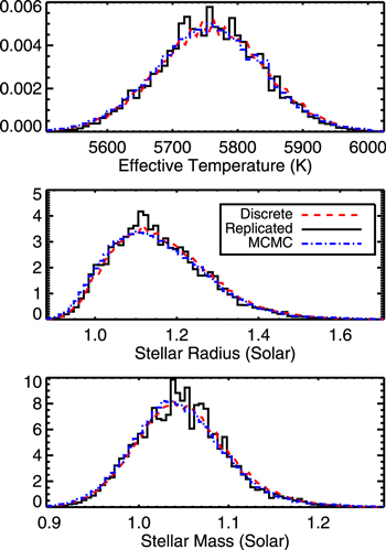
Figure 5. Comparison of replicated posteriors (black solid lines), discrete posteriors (red dashed lines), and MCMC posteriors (blue dot–dashed lines) for the temperature, radius, and mass of Kepler-452. The MCMC posteriors were taken from Jenkins et al. (2015).
Download figure:
Standard image High-resolution imageFigure 6 shows an example comparison between discrete posteriors and replicated posteriors for a typical solar-type dwarf in the Kepler sample with a photometric input  . The replicated posteriors again show good agreement with the discrete posteriors, even in the case of bimodal distributions. We checked the results for different spectral types, which looked similar to this example.
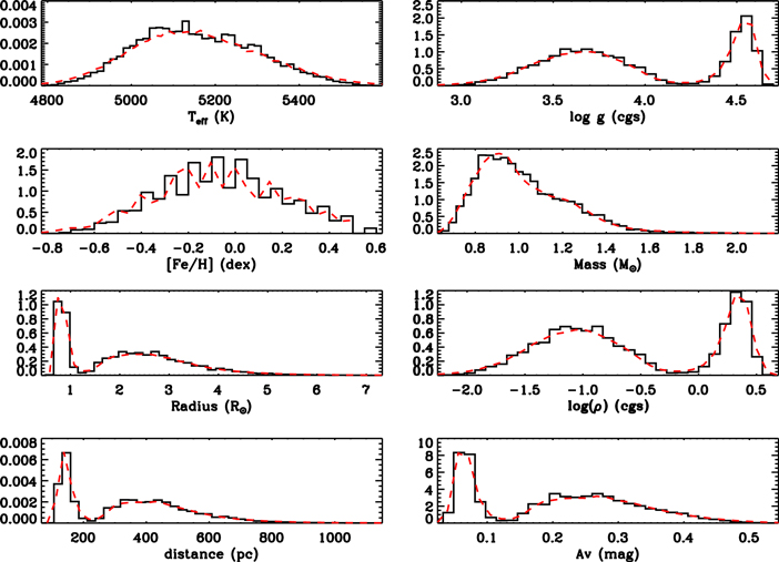
Figure 6. Comparison of replicated posteriors (black solid lines) and discrete posteriors (red dashed line) for a typical solar-type star in the Kepler sample, KIC 757076 (Kp = 11.7). The input values for  ,
,  , and [Fe/H] are PHO1, KIC, and KIC respectively.
Download figure:
Standard image High-resolution image4. Final Catalog Description
Applying the method described above to all stars in Table 3 yielded best-fit values and 1σ confidence intervals for mass, radius, surface gravity, effective temperature, density, metallicity, distance, and extinction for all 197,096 stars, which are listed in Table 4. Each entry also gives the origin of the input values used for  ,
,  , and [Fe/H] as described in Section 2.2. Finally, for each star we give the provenance for the derived parameters. While most of the stars have their output parameters derived from the isochrone fitting method of Section 3.1 (abbreviation DSEP), for 235 stars we used previously published values for cool dwarfs and for stars falling off the isochrone grid (see Section 5.3 for more details). For this small sample of stars, distances and extinctions are not given and their provenance is BTSL since the parameters were estimated from polynomial fits to low-mass BT-Settl models (Allard et al. 2012). The abbreviation MULT corresponds to parameters derived from multiple evolutionary tracks and is given to a handful of stars. With these flags, the reference(s) of the input values and the method used to derive the stellar parameters can be traced. We note that unlike previous catalog deliveries, we did not override published solutions that provide better estimates for radii and masses (e.g., from asteroseismology) in order to homogeneously derive stellar properties (including distances) for all stars. This means that better estimates for radii and masses may be available in the literature for some stars.
The full catalog is available at the NASA exoplanet archive17
along with the replicated posteriors obtained as described in Section 3.2. Note that the online catalog contains 200,038 entries. The difference between the number of stars with derived parameters (197,096) and the total number of Kepler targets during the whole mission comes from the fact that 2942 stars are still unclassified without any  ,
,  , and [Fe/H] available. Of these stars, 139 only had Q0 observations, 528 stars were only observed in Q17, 8 are flagged as a galaxy, and 516 stars do not have valid 2MASS photometry. We also note that 1800 of these unclassified stars are faint (
 ).
).
5. Discussion
5.1. Quality Control Tests
5.1.1. Comparison of Input and Output Values
The first quality control test was to compare the input and output values for a well-characterized sample of stars that have asteroseismic gravities or spectroscopic effective temperatures. Large deviations between input and output  or
or  values may indicate potential misclassifications due to problems with the adopted input values or the isochrone fitting method.
Asteroseismic gravities are available for 16,947 stars (red giants and dwarfs), while spectroscopic temperatures were obtained for 14,813 stars. Figure 7 shows the difference between the input values of  and
and  and the DR25 values for the subsample of these stars. For
  most of the output values agree with the seismic values within 1σ, and 5 stars disagree by more than 1σ. The largest disagreement concerns stars with
  values between 2 and 3, i.e., red giants including red clump stars. This can be explained by the fact that the DSEP models do not include helium-burning red giant models, as pointed out by H14.
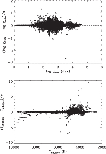
Figure 7. Top panel: differences between input and output  values in units of σ for stars with asteroseismic input values for
  . The adopted typical uncertainty for asteroseismic
  values is 0.03 dex. Bottom panel: same as top panel, but for stars with spectroscopic
  . The adopted uncertainty is 2%.
Download figure:
Standard image High-resolution imageThe effective temperature comparison (bottom panel of Figure 7) shows that in most cases the values provided in the catalog agree with the spectroscopic input values within 1σ. A large number of stars with  between 3500 and 5500 K disagree by more than 1σ. These stars are again mostly red giants. We note that 11 stars disagree by more than 5σ. Of these, 3 stars (KIC 8714886, 10536147, and 10797526) have Teff > 15,000 K, well beyond our grid of models (and out of the plot), therefore we report their DR24 stellar parameters for which the effective temperatures are close to 16,000 K. The remaining 9 stars have input values that are slightly off the model grid, thus the code converges to the parameter space that is significantly different than the input values. Three of these stars (KIC 2585447, 3968716, and 8559125) are new red giants with seismic
  and spectroscopic
  . The first 2 stars are flagged in Mathur et al. (2016) as a possible blend. This means that either the oscillation detection comes from another close-by star or that the blend has an impact on the estimate of the effective temperature in the spectroscopic analysis. KIC 8559125 is not a misclassified red giant anymore, as it was removed from the list after the delivery of the DR25 catalog, as explained in Section 5.3. The last 5 stars (KIC 3335176, 3346584, 4078024, 4263398, and 8710336) have seismic and/or spectroscopic input values, but are slightly off the grid, which explains the large difference between the input and the output values.
5.1.2. Comparison to Previous Catalogs
Figure 8 shows the surface gravity versus temperature distribution for DR25 (left panel) and DR24 (right panel). It is evident that the DR25 catalog contains a significantly larger fraction of subgiants, mostly because the LAMOST and Flicker surface gravities are included. Using Equations (8) and (9) from Huber et al. (2016), we computed the number of subgiants and found that DR25 contains 15,893 subgiants compared to 11,078 in DR24, an increase of 43.5%. While these updates generally only affect the brighter Kepler targets ( ), this indicates that the DR25 catalog should be less prone to the systematic underestimation of radii for solar-type dwarfs than previous catalogs.
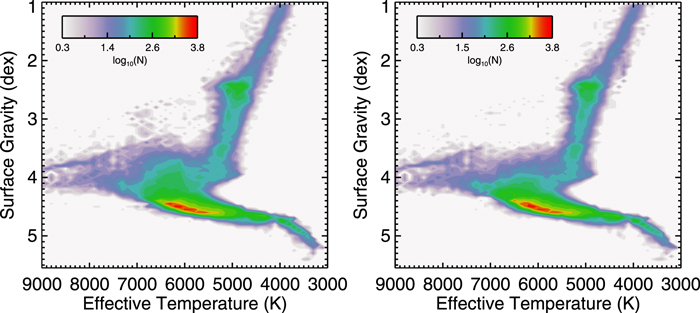
Figure 8. Surface gravity vs. effective temperature for all classified stars in this catalog (DR25, left panel) and the previous catalog (DR24, right panel). Color denotes the logarithmic number density of stars.
Download figure:
Standard image High-resolution imageFigures 9 and 10 show the ratios of DR24 to DR25 radii and masses. These plots represent the logarithm of the number density of stars for different effective temperatures and gravity bins. Figures 9 and 10 are included for all stars (upper left) as well as the samples highlighted in Section 2.2.
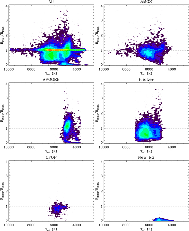
Figure 9. Ratio of radii from DR24 and DR25 for the full sample (top left panel), the LAMOST sample (top middle panel), the APOGEE sample (top right panel), the sample with Flicker  (bottom left panel), the sample of stars with CFOP spectroscopy (bottom middle panel), and the sample of new red giants (bottom right panel). Color denotes the number density of stars.
Download figure:
Standard image High-resolution image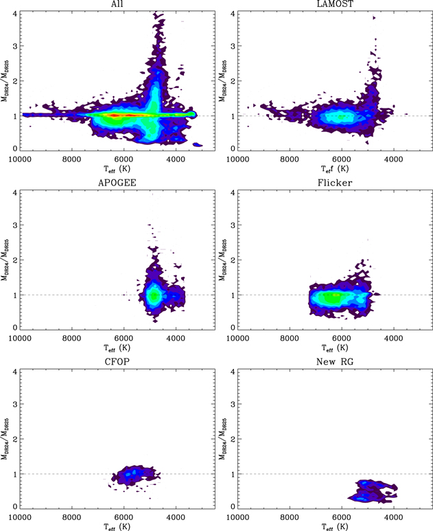
Figure 10. Same as Figure 9, but for stellar mass.
Download figure:
Standard image High-resolution imageFigure 9 shows that the highest density of stars is close to the  line, which means that their radii did not change. The stars with the most significant changes in the stellar parameters correspond to stars with new input values, as expected. Stars with LAMOST and Flicker inputs have a larger number density of stars slightly below the ratio equals 1 line, which means that these stars have become larger (up to a factor of 2). Stars with APOGEE inputs are on both sides of the 1 line with higher number density above 1 (i.e., smaller radii in the DR25). Finally, the new red giants have a radius ratio close to 0, corresponding to a large increase of the size of the star from a dwarf to a red giant. Some of these cases are also present in the APOGEE sample.
The mass comparison also shows that the highest number density of stars is close to 1:1 line. Stars with Flicker and CFOP inputs see their masses change by less than a factor of 2. The new inputs from LAMOST and APOGEE show a similar behavior, except that they also lead to lower masses for stars with  K.
K.
In both Figures 9 and 10 we see a group of cool stars ( ) that systematically fall below the 1:1 line. These are stars that were erroneously classified as giants in the H14 catalog and corrected using the dwarf classifications by Mann et al. (2012) in the DR25 catalog, as further explained in Section 5.3.
After completion of DR25 catalog, Gaidos et al. (2016, hereafter G16) published the revised properties of 4216 M dwarfs observed by Kepler. A total of 699 stars in G16 are not included in the DR25 catalog since they were only observed during Q17 and had neither KIC values available nor spectroscopic inputs. For 68 stars spectroscopic parameters were also published by Frasca et al. (2016). For the stars in common between G16 and DR25, the two temperature scales are close for cool stars below 3500 K, although the temperatures from G16 are on average 200 K hotter for 63 stars. Above 3500 K, the temperatures from G16 are cooler compared to the DR25 values, with differences larger than 200 K (up to 2000 K) for 487 stars. We found that 54 stars in G16 are classified as red giants in the DR25. A small sample of these stars (16) were classified as red giants from seismology, which means that the detection of oscillations does not agree with the dwarf classification of G16. A majority of the stars with DR25 temperatures hotter than 4000 K have a  provenance from the KIC and PHO54. Given that the analysis by G16 was specifically tailored toward cool dwarfs, some of these stars may be misclassified in the DR25 catalog, and hence the classifications by G16 should be preferred over the DR25 catalog. We list these potentially misclassified stars in Appendix
5.1.3. Effects on Planet Host Star Parameters
As a final test, we looked in particular at planet host star parameters as they directly affect the size inferred for the planets. Figure 11 compares the radii and masses of the planet host stars computed in this work with the DR24 catalog. It is encouraging to see that stars for which we used the same inputs as the DR24 catalog (black diamonds in the figure) fall on or are very close to the line  /
/ , indicating that the radii of these stars changed by a few percent at most. The small change can be explained by the updated isochrone grid that was used in this work.
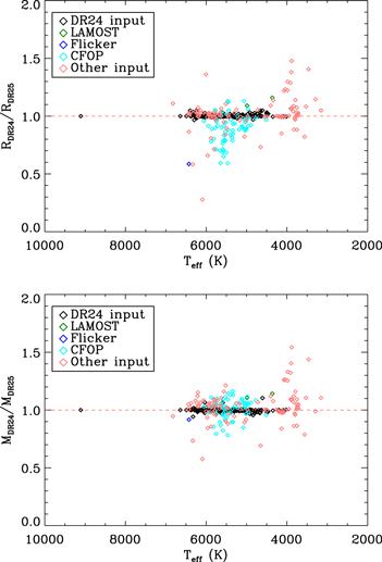
Figure 11. Comparison of radii and masses of planet host stars showing the different subsamples for which we used either new inputs values or the same input values as in the previous catalog.
Download figure:
Standard image High-resolution imageAs expected, the largest changes are visible for stars with new input values. Many stars with new CFOP parameters have a different evolutionary stage. We described above that a fraction of stars moved from main-sequence stars to more evolved subgiants. This explains the number of stars that now have a larger radius than in the previous catalog (cyan symbols). This is also the case for the star with the Flicker input (blue symbol) and some of the individual new inputs (pink symbols).
For stars cooler than 4500 K, we note that a significant number of host stars become smaller and less massive. Specifically, for eight host stars the spectroscopic classification by Rowe et al. (2014) was subsequently shown to lead to systematically overestimated effective temperatures and radii and hence led to biased estimates in the DR24 catalog. To correct this, we adopted the inputs from H14 for these stars for the DR25 catalog.
The following is a list of specific host stars with significant changes in their stellar parameters:
- (1)The radii of the K-dwarfs KIC 5640085 (KOI-448 and Kepler-148) and KIC 10027323 (KOI-1596 and Kepler-309) decreased by ∼40%–50% due to the correction of the spectroscopic input values from Rowe et al. (2014), as discussed above. The input parameters were reversed back to those in the H14 catalog, which were based on Muirhead et al. (2012a).
- (2)KIC 7529266 (KOI-680, Kepler-635) is a solar-type star (∼6000 K) and shows the largest change in radius ( ∼ 0.3). We adopted updated input values from Almenara et al. (2015), who listed a of 3.5 dex compared to 4.35 dex in the KIC, leading to a large increase in radius. It is not surprising to see this change given that the original KIC had known shortcomings regarding the classification of subgiants.
- (3)


5.2. Distances and Extinction
In addition to stellar parameters, the DR25 catalog also includes distances and extinction values for ∼196,850 stars (see Section 5.3 for more details). Figure 12 shows the distribution of distances for dwarfs (left panel) and for red giants (right panel) observed by Kepler. As expected, red giants observed by Kepler are on average more distant than dwarfs.
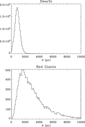
Figure 12. Distribution of distances for dwarfs (top panel) and red giants (bottom panel) in the DR25 catalog.
Download figure:
Standard image High-resolution imageWe also compared our catalog distances to Rodrigues et al. (2014, hereafter R14), who combined asteroseismology with APOGEE spectra to derive distances and extinctions for a sample of ∼2000 Kepler red giants. The comparison showed that the catalog distances are systematically larger by up to 50%, the reason for which is that our model grid does not include He-core burning models for low-mass stars, and hence giants are preferentially fitted to models with higher mass that are more luminous and hence more distant. This bias has been pointed out in H14 and should be kept in mind when using catalog results for red giant stars. We emphasize that this distance bias is not expected to be relevant for dwarfs and subgiant stars, which form the majority of the Kepler target sample.
Finally, a comparison of extinction values to Rodrigues et al. (2014) showed that the catalog values for giants are systematically higher by ∼0.1–0.3 mag on average, similar to the results found for the KIC (see Figure 17 of R14). This is most likely due to the simplified 3D reddening model adopted in this work and the KIC compared to the method adopted by R14, which derives reddening values by comparing synthetic to observed photometry on a star-by-star basis. Since this method is only effective if  ,
,  , and
, and ![$[\mathrm{Fe}/{\rm{H}}]$](https://content.cld.iop.org/journals/0067-0049/229/2/30/revision1/apjsaa567bieqn206.gif) can be derived independently from photometry, it cannot be applied to the full Kepler sample at this point.
can be derived independently from photometry, it cannot be applied to the full Kepler sample at this point.
5.3. Catalog Shortcomings
While this paper provides important improvements over previous Kepler stellar properties catalogs, several shortcomings remain. In particular:
- 1.For stars with input values that fall off the Dartmouth isochrone grid (e.g., very cool dwarfs) we adopted the input and output values from H14. There are also three stars where we adopted the published values (KIC 5807616, 5868793 and 10001893). These three stars fall out of the grid because they are too hot, with a temperature above 25,000 K. These stars do not have distances and extinction values. The provenance for the mass, radius, and density is MULT as they come from a different method.
- 2.Unlike in previous deliveries, we did not override catalog values with published solutions that provide better estimates for radii and masses (e.g., from asteroseismology) in order to homogeneously derive posterior distributions (including distances) for all stars. This means that better estimates for radii and masses may be available in the literature for some stars.
- 3.Similar to H14, the adopted isochrone grid does not include He-core burning models for low-mass stars, and hence derived properties for red giants (such as radius, mass, and distances) will be systematically biased toward higher-mass stars (and more distant for red giants). Users are strongly encouraged to adopt values from dedicated Kepler red giant classification programs such as the APOKASC (e.g., Pinsonneault et al. 2014) or SAGA (Casagrande et al. 2014) surveys for these stars, or use the provided, , and values in this catalog as input for deriving more accurate stellar properties.
- 4.The new catalog also includes several corrections that were pointed out by the community since the release of the H14 catalog. Owing to a coding error, every star in the Q1–16 catalog with input was automatically classified as a dwarf using BT-Settl models even if the input indicated that it was a giant. To correct this, we revisited all dwarfs that have been classified using BT-Settl models and verified their evolutionary state using the Mann et al. (2012) spectroscopic classifications. When this was verified, we adopted the Q1–16 BT-Settl solution. These stars do not have distances and extinction values. The provenance for the mass, radius, and density is BTSL.
- 5.The number of misclassified red giants reported in Mathur et al. (2016) is 854, while in this delivery the misclassified red giants represent 835 stars. Between the delivery of the catalog and the finalization of the misclassified red giants, some stars were dropped because they were polluted by nearby known red giants, while others were added. This explains the discrepancy of 51 stars.
- 6.For the vast majority of targets the input classifications assumed that all the stars are single systems, which can lead to biased stellar parameters when the targets are in fact multiple star systems. While we expect that this effect is small compared to the typical uncertainties in the derived stellar properties, future catalog releases will attempt to take information from various high-resolution imaging programs into account (e.g., Adams et al. 2012; Dressing et al. 2014; Lillo-Box et al. 2014; Baranec et al. 2016; Furlan et al. 2016; Kraus et al. 2016) for stellar classifications.


![$[\mathrm{Fe}/{\rm{H}}]$](https://content.cld.iop.org/journals/0067-0049/229/2/30/revision1/apjsaa567bieqn209.gif)


6. Summary
The DR25 Kepler stellar properties catalog includes improved stellar properties for over 28,800 stars, including spectroscopic surveys (CFOP, APOGEE, and LAMOST),  values derived from stellar granulation (Flicker), and new asteroseismic reclassifications of more than 800 stars (Mathur et al. 2016). We also added 311 stars that were targeted during the last quarter observed by Kepler, Q17. Finally, 317 stars that had not been classified so far were included in this catalog using spectroscopic classifications from LAMOST and APOGEE. This leads to a total number of stars in the Kepler DR25 catalog of 197,096, including 4085 planet(-candidate) host stars. The DR25 stellar properties catalog has been used for the final Transiting Planet Search/Data Validation (TPS/DV) by the Kepler Mission, and is available at the NASA Exoplanet Archive (http://exoplanetarchive.ipac.caltech.edu) and the Mikulski Archive for Space Telescopes (MAST, http://archive.stsci.edu/kepler/stellar17/search.php). We note that there are still ∼3000 unclassified stars that do not have reliable colors and were not analyzed in this work. A major addition compared to the DR24 catalog is the delivery of the posterior samples for all stellar parameters for ∼196,850 stars.
The catalog was constructed with a method similar as in H14, using input data from different techniques such as asteroseismology, spectroscopy, photometry, or Flicker. The effective temperature, surface gravity, and metallicity were then conditioned on a grid of isochrones to provide posterior distributions of all parameters. While the input values still come from a variety of sources, the updated method in principle allowed a homogeneous estimation of all derived quantities such as mass, radius, density, distance, and extinction. The update of the method from the H14 catalog also led to slightly smaller and more realistic uncertainties associated with the stellar parameters. However, we emphasize that there are still a number of significant shortcomings in the catalog, as described in Section 5.3. We also note that distances and extinctions listed in this paper are systematically different from the values in the original delivery to the NASA Exoplanet archive because of the coding error explained in Section 3.3. All other stellar properties are unaffected, but we recommend using the corrected distances listed in this paper for scientific investigations of the Kepler sample.
Even though the DR25 catalog forms the basis for the final TPS in the Kepler mission close-out, the improvement in the characterization of all Kepler targets will continue to develop in the coming years. Indeed, since the delivery of the catalog additional observations and analyses have been performed for Kepler targets. For example, Gaidos et al. (2016) obtained spectra for more than 3000 dwarfs and provided more accurate  and
and  . More recently, Yu et al. (2016) used asteroseismology to reclassify more than 1500 subgiants in DR25 as red giants. Finally, the most important update of the Kepler stellar properties catalog can be expected with the advent of high-precision parallaxes by the ESA Gaia mission (Perryman 2005), for which the first data release has been announced (Gaia Collaboration et al. 2016). These parallaxes will at last provide an efficient tool to precisely determine the evolutionary states of nearly all targets observed by Kepler.
The authors would like to thank Michael Haas and Eric Gaidos for useful discussions. S.M. would like to thank R. A. García and the CEA Saclay (France) for their computing resources. S.M. and D.H. acknowledge support by the National Aeronautics and Space Administration under Grant NNX14AB92G issued through the Kepler Participating Scientist Program, and D.H. acknowledges support by the Australian Research Council’s Discovery Projects funding scheme (project number DE140101364). F.B. is supported by NASA through Hubble Fellowship grant #HST-HF2-51335 awarded by the Space Telescope Science Institute, which is operated by the Association of Universities for Research in Astronomy, Inc., for NASA, under contract NAS5-26555.
Appendix A: Provenances of Input Parameters
We followed the same scheme as introduced by H14 to numerically cross-link literature sources of input parameters to a given provenance (see Section 6.5 in H14). Table 5 lists the complete references for all input sources used in the DR25 catalog. As an example, a  provenance of AST10 indicates that the input
  value was derived from asteroseismology and taken from Chaplin et al. (2014).
Table 5. Reference Key
| Key | References | Method |
|---|---|---|
| 0 | Brown et al. (2011) | Photometry |
| 1 | Pinsonneault et al. (2012) | Photometry |
| 2 | Dressing & Charbonneau (2013) | Photometry |
| 3 | Buchhave et al. (2012) | Spectroscopy |
| 4 | Uytterhoeven et al. (2011) | Spectroscopy |
| 5 | Muirhead et al. (2012a) | Spectroscopy |
| 6 | Bruntt et al. (2012) | Spectroscopy/Asteroseismology |
| 7 | Thygesen et al. (2012) | Spectroscopy/Asteroseismology |
| 8 | Huber et al. (2013) | Spectroscopy/Asteroseismology |
| 9 | Stello et al. (2013) | Asteroseismology |
| 10 | Chaplin et al. (2014) | Asteroseismology |
| 11 | Huber et al. (2011) | Asteroseismology |
| 12 | Petigura et al. (2013b) | Spectroscopy |
| 13 | Molenda-Żakowicz et al. (2013) | Spectroscopy |
| 14 | Mann et al. (2012) | Spectroscopy |
| 15 | Mann et al. (2013b) | Spectroscopy |
| 16 | Gaidos (2013) | Photometry |
| 17 | Martín et al. (2013) | Spectroscopy |
| 18 | Batalha et al. (2013) | Spectroscopy/Transits |
| 19 | White et al. (2013) | Spectroscopy/Asteroseismology |
| 20 | Bakos et al. (2010) | Spectroscopy/Transits/EBs |
| 21 | Koch et al. (2010) | Spectroscopy/Transits/EBs |
| 22 | Dunham et al. (2010) | Spectroscopy/Transits/EBs |
| 23 | Jenkins et al. (2010) | Spectroscopy/Transits/EBs |
| 24 | Holman et al. (2010) | Spectroscopy/Transits/EBs |
| 25 | Lissauer et al. (2013) | Spectroscopy/Transits/EBs |
| 26 | Fortney et al. (2011) | Spectroscopy/Transits/EBs |
| 27 | Endl et al. (2011) | Spectroscopy/Transits/EBs |
| 28 | Doyle et al. (2011) | Spectroscopy/Transits/EBs |
| 29 | Désert et al. (2011) | Spectroscopy/Transits/EBs |
| 30 | Cochran et al. (2011) | Spectroscopy/Transits/EBs |
| 31 | Ballard et al. (2011) | Spectroscopy/Transits/EBs |
| 32 | Fressin et al. (2012) | Spectroscopy/Transits/EBs |
| 33 | Steffen et al. (2012) | Spectroscopy/Transits/EBs |
| 34 | Fabrycky et al. (2012) | Spectroscopy/Transits/EBs |
| 35 | Lissauer et al. (2012) | Spectroscopy/Transits/EBs |
| 36 | Welsh et al. (2012) | Spectroscopy/Transits/EBs |
| 37 | Orosz et al. (2012a) | Spectroscopy/Transits/EBs |
| 38 | Bouchy et al. (2011) | Spectroscopy/Transits/EBs |
| 39 | Santerne et al. (2011b) | Spectroscopy/Transits/EBs |
| 40 | Santerne et al. (2011a) | Spectroscopy/Transits/EBs |
| 41 | Muirhead et al. (2012b) | Spectroscopy/Transits/EBs |
| 42 | Bonomo et al. (2012) | Spectroscopy/Transits/EBs |
| 43 | Johnson et al. (2012) | Spectroscopy/Transits/EBs |
| 44 | Nesvorný et al. (2012) | Spectroscopy/Transits/EBs |
| 45 | Orosz et al. (2012b) | Spectroscopy/Transits/EBs |
| 46 | Ballard et al. (2013) | Spectroscopy/Transits/EBs |
| 47 | Meibom et al. (2013) | Spectroscopy/Transits/EBs |
| 48 | Barclay et al. (2013) | Spectroscopy/Transits/EBs |
| 49 | Charpinet et al. (2011) | Spectroscopy/Transits/EBs |
| 50 | Howell et al. (2010) | Spectroscopy/Transits/EBs |
| 51 | Hébrard et al. (2013) | Spectroscopy/Transits/EBs |
| 52 | Faigler et al. (2013) | Spectroscopy/Transits/EBs |
| 53 | Sanchis-Ojeda et al. (2013) | Spectroscopy/Transits/EBs |
| 54 | Huber et al. (2014) | Photometry/Asteroseismology |
| 55 | Pinsonneault et al. (2014) | Photometry/Asteroseismology/Spectroscopy |
| 56 | Casagrande et al. (2014) | Photometry/Asteroseismology |
| 57 | Petigura et al. (2013a) | Spectroscopy |
| 58 | Rowe et al. (2014) | Spectroscopy |
| 59 | Buchhave et al. (2014) | Spectroscopy |
| 60 | Mann et al. (2013b, 2013a) | Spectroscopy |
| 61 | Marcy et al. (2014) | Spectroscopy |
| 62 | Borucki et al. (2013) | Spectroscopy |
| 63 | Sanchis-Ojeda et al. (2013) | Spectroscopy |
| 64 | Gandolfi et al. (2013) | Spectroscopy/Transits |
| 65 | Ofir et al. (2014) | Spectroscopy/Transits |
| 66 | Deleuil et al. (2014) | Spectroscopy/Transits |
| 67 | Tingley et al. (2014) | Spectroscopy |
| 68 | Luo et al. (2015) | Spectroscopy |
| 69 | Silva Aguirre et al. (2015) | Spectroscopy/Asteroseismology |
| 70 | Muirhead et al. (2014) | Spectroscopy |
| 71 | Mathur et al. (2016) | Asteroseismology |
| 72 | W. J. Chaplin et al. (2017, in preparation) | Spectroscopy |
| 73 | Bastien et al. (2016) | Flicker |
| 74 | Alam et al. (2015) | Spectroscopy |
| 75 | Mancini et al. (2016) | Spectroscopy |
| 76 | Almenara et al. (2015) | Spectroscopy |
| 77 | Hébrard et al. (2014) | Spectroscopy |
| 78 | Santerne et al. (2014) | Spectroscopy |
| 79 | Dawson et al. (2014) | Spectroscopy |
| 80 | Kipping et al. (2014) | Spectroscopy |
| 81 | Endl et al. (2014) | Spectroscopy |
| 82 | Gandolfi et al. (2015) | Spectroscopy |
| 83 | Silvotti et al. (2014) | Spectroscopy |
| 84 | Everett et al. (2015) | Spectroscopy |
| 85 | Torres et al. (2015) | Spectroscopy |
| 86 | Muirhead et al. (2015) | Spectroscopy |
| 87 | Lillo-Box et al. (2015) | Spectroscopy |
| 88 | Bourrier et al. (2015) | Spectroscopy |
| 89 | Borucki et al. (2012) | Spectroscopy |
| 90 | E. Furlan et al. (2017, in preparation) | Spectroscopy |
Download table as: ASCIITypeset image
Appendix B: Stellar Replicated Posteriors
The DR25 catalog delivery includes replicated posteriors for each star obtained as described in Section 3.4. The files contain 40,000 samples of self-consistent stellar parameters, together with the logarithm of total likelihood and the isochrone weights, corresponding to the volume of each model in mass, metallicity, and age. Age, mass, and metallicity priors are not listed as we used uniform priors for these quantities.
Replicated posterior files have the generic name “kplr < kepler id > dr25-stellarposterior.txt” and contain 10 space-separated columns for each star:  ,
,  , [Fe/H], mass, radius,
  , distance, Av, log(likelihood), and log(weights). Each row corresponds to a set of self-consistent stellar properties and can therefore be used to produce marginalized distributions or explore parameter correlations. Figure 13 shows an example of parameter correlations for KIC 757076, which has a best-fit
  and
and  in DR25.
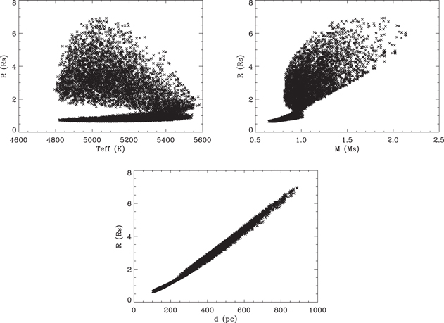
Figure 13. Example of correlations between posterior samples for KIC 757076: radius vs.  (top left), radius vs. mass (top right), and radius vs. distance (bottom).
Download figure:
Standard image High-resolution imageAppendix C: Possible Misclassified M Dwarfs
As discussed in Section 5.1.2, 54 targets that are classified as giants in the DR25 catalog have been classified as cool dwarfs by G16. Since these targets are potentially interesting for planet searches, we list them in Table 6 together with the listed 
 and R values in both catalogs. We note that follow-up spectroscopy will be needed to unambiguously determine the evolutionary state for these stars.
Table 6. Possible M Dwarfs According to Gaidos et al. (2016)
| KIC |
 (K) (K) |

|
R* (R⊙) |
 (K) (K) |

|
R (R⊙) |

|
Plog g |
|---|---|---|---|---|---|---|---|---|
| 1575570 | 3429 | 4.89 | 0.36 | 3370 | 0.46 | 175.79 | KIC0 | KIC0 |
| 3629762 | 3241 | 5.04 | 0.25 | 3279 | 0.16 | 151.95 | KIC0 | KIC0 |
| 4454364 | 3586 | 4.87 | 0.38 | 4102 | 1.61 | 25.69 | PHO2 | AST71 |
| 4466520 | 3385 | 4.89 | 0.36 | 3500 | 0.66 | 147.76 | KIC0 | KIC0 |
| 4473475 | 3449 | 4.92 | 0.34 | 4477 | 2.33 | 10.90 | PHO2 | AST71 |
| 4732678 | 3963 | 4.66 | 0.62 | 3683 | 0.73 | 92.23 | PHO54 | AST54 |
| 5122206 | 3359 | 4.96 | 0.30 | 3400 | 0.50 | 179.17 | KIC0 | KIC0 |
| 5446961 | 3676 | 4.68 | 0.59 | 4487 | 2.93 | 5.62 | KIC0 | AST71 |
| 5471005 | 3965 | 4.59 | 0.72 | 4297 | 1.78 | 26.80 | PHO54 | AST54 |
Note.  ,
,  , and R* are the effective temperature, surface gravity, and radius from G16.
  ,
,  , and R are the effective temperature, surface gravity, and radius from DR25.
  and Plog g are the provenances of
  and
and  in DR25 as described in Table 5.
Only a portion of this table is shown here to demonstrate its form and content. A machine-readable version of the full table is available.
Download table as: DataTypeset image
Footnotes
- 16
- 17