Abstract
Optical depth variations in the Galactic neutral interstellar medium (ISM) with spatial scales from hundreds to thousands of astronomical units have been observed through H i absorption against pulsars and continuum sources, while extremely small structures with spatial scales of tens of astronomical units remain largely unexplored. The nature and formation of such tiny-scale atomic structures (TSAS) need to be better understood. We report a tentative detection of TSAS with a signal-to-noise ratio of 3.2 toward PSR B1557−50 in the second epoch of two Parkes sessions just 0.36 yr apart, which are the closest-spaced spectral observations toward this pulsar. One absorption component showing marginal variations has been identified. Based on the pulsar’s proper motion of 14 mas yr−1 and the component’s kinematic distance of 3.3 kpc, the corresponding characteristic spatial scale is 17 au, which is among the smallest sizes of known TSAS. Assuming a similar line-of-sight (LOS) depth, the tentative TSAS cloud detected here is overdense and overpressured relative to the cold neutral medium (CNM), and can radiatively cool fast enough to be in thermal equilibrium with the ambient environment. We find that turbulence is not sufficient to confine the overpressured TSAS. We explore the LOS elongation that would be required for the tentative TSAS to be at the canonical CNM pressure, and find that it is ∼5000—much larger than filaments observed in the ISM. We see some evidence of line width and temperature variations in the CNM components observed at the two epochs, as predicted by models of TSAS-like cloud formation colliding warm neutral medium flows.
1. Introduction
Tiny-scale atomic structures (TSAS) with spatial scales spanning from a few to hundreds of astronomical units have been studied for over four decades in the interstellar medium (ISM). Compared to the traditional definitions of the atomic medium in thermal equilibrium states—the cold neutral medium (CNM) and the warm neutral medium (WNM)—TSAS are overdense and overpressured, with densities and pressures several orders of magnitude higher than the theoretical values based on the heating and cooling balance (Stanimirović & Zweibel 2018). TSAS has been probed mainly through three methods: (1) spatial and temporal H i absorption variability from high-resolution maps against extragalactic compact and resolved radio continuum sources (e.g., Diamond et al. 1989; Deshpande et al. 2000; Lazio et al. 2009; Roy et al. 2012; Rybarczyk et al. 2020); (2) temporal variability of H i absorption against pulsars (e.g., Frail et al. 1994; Johnston et al. 2003; Minter et al. 2005; Stanimirović et al. 2010); (3) spatial and temporal absorption variability of optical and ultraviolet lines (e.g., Na i, Ca i) toward stars in binary, multiple stellar systems, and globular clusters over a period of years (e.g., Meyer 1990; Meyer & Blades 1996; Lauroesch & Meyer 2003).
Several mechanisms have been proposed to form TSAS, although there is no consensus yet. These mechanisms include TSAS being the tail-end of the turbulent spectrum (Deshpande et al. 2000), discrete elongated disk or cylinder clouds passing across the line of sight (Heiles 1997), isolated events, such as fragmentation of the Local Bubble wall through hydrodynamic instabilities (Stanimirović et al. 2010), and structures related to planet-building gas materials (Ray & Loeb 2017; Stanimirović & Zweibel 2018). If TSAS represents the tail-end of turbulent dissipation processes, then a power-law relation between the spatial scales of TSAS and the optical depth variation is expected (Deshpande 2000). Alternatively, Koyama & Inutsuka (2002) and Hennebelle & Audit (2007) modeled TSAS creation by shocks and colliding WNM flows in shocked regions.
Pulsars are particularly useful background sources because: (1) on- and off-source measurements can be obtained without position switching; (2) the relative high-velocity motion of the Earth and a pulsar over time allows us to sample a slightly different line of sight (LOS) through the ISM, therefore probing small structures in the ISM; (3) H i absorption spectra of low-latitude pulsars can be used to estimate the pulsar kinematic distance (Weisberg et al. 2008);
TSAS may contain ionized gas. For example, assuming shielding is not too high, a high fraction of the carbon in TSAS clouds may be ionized by the interstellar radiation field (Heiles 1997; Stanimirović & Zweibel 2018). Ionization of hydrogen may also be instigated by local stellar objects, to produce fully ionized tiny-scale structures. McCullough & Benjamin (2001) detected an extremely narrow ionized filament, which can be attributed to the effect of photoionization from a star or compact object. Tiny-scale inhomogeneities in the ionized ISM can also be discerned through scintillation and/or extreme scattering events (Stanimirović & Zweibel 2018). For example, Basu et al. (2016), Coles et al. (2015), and Hill et al. (2005) detected tiny-scale ionized structure with spatial scales of a few to hundreds of astronomical units through extreme scattering events and substructure in scintillation arcs toward pulsars.
PSR B1557−50 (J1600−5044) was the first pulsar against which H i absorption variations were detected in the southern sky (Deshpande et al. 1992). In observations spaced around five years apart, these authors found an overpressured TSAS with a spatial scale of 1000 au, at a velocity of −40 km s−1 with Δτ of 1.1. Johnston et al. (2003) confirmed similar H i absorption variation at −40 km s−1 as well as another two components at −110 and −80 km s−1 toward this pulsar using Parkes, in two observational epochs spaced 14 yr apart. They concluded that the component at −110 km s−1 is related to a TSAS of 1000 au, with a density of 2.6 × 104 cm−3, and Δτ of 0.15. The sight line toward PSR B1557−50 traverses substantial distances, and has previously been monitored at such long cadences that multiple TSAS components could have passed across the source between observations. We focus here on monitoring PSR B1557−50 over a much shorter time baseline: ∼0.36 yr.
This Letter is organized as follows: Section 2 describes the observing and data processing strategies. In Section 3, we decompose the optical depth profile and study the properties of the CNM. Meanwhile, we analyze the variations of H i optical depth profiles and the properties of the changes in the observed H i gas at different epochs. We discuss our results and their implications in Section 4. We conclude in Section 5.
2. Observations and Data Processing
We used the Parkes ultra-wide-bandwidth, low-frequency receiver (“UWL”) and the MEDUSA signal processing system (Hobbs et al. 2020) to observe the 21 cm H i line toward PSR B1557−50 at two epochs, referred to below as E1(2019.42) and E2(2019.78). The UTC dates at the beginning of the observations are 2019 May 26 and 2019 September 11, respectively. The integration time for each epoch was 379 and 382 minutes, respectively.
We recorded voltage data streams covering frequencies from 1344 to 1472 MHz. We injected a calibration signal (CAL) every 1 hr for a duration of 3 minutes in order to calibrate the antenna temperature. We used the DSPSR package (van Straten & Bailes 2011) to process the baseband data to get spectra with a velocity resolution of ∼0.1 km s−1. The data were folded synchronously with the pulsar period for an integration time of 10 s with 64 phase bins.
The pulse profile for each polarization is generated by collapsing (after de-dispersion) the data along the frequency dimension, which gives the location of pulsar-on and pulsar-off phase bins. The pulsar-on and pulsar-off spectra were obtained based on the strategies described by Weisberg et al. (2008). The absorption spectrum is the difference of the pulsar-on and pulsar-off spectra on an antenna temperature scale, I(v) = Ion(v) − Ioff(v). The final normalized absorption spectrum (I(v)/I0) was obtained by dividing the final absorption spectrum by the mean value excluding the absorption channels (I0). According to radiative transfer, the pulsar-on and pulsar-off spectra can be written as

where Tbg is the background brightness temperature, τv is the H i optical depth, Ts is the H i spin temperature, and Tpsr is the pulsar continuum brightness temperature. Therefore,

The final calibrated antenna temperature of the H i emission spectrum, TH I(v), is required to compute the frequency-dependent noise spectrum (see Section 3.2). TH I(v) was obtained by removing the baseline of Ioff(v) using a third-order polynomial. To obtain the brightness temperature-calibrated Toff(v), which is required to derive Ts (see Appendix B), we scaled TH I(v) to match the Parkes Galactic All-Sky Survey (GASS) intensity scale (McClure-Griffiths et al. 2009).
The absorption spectra are affected by on-source ripples, especially for E2. We identified the Fourier components of the ripples. Among these there are two baseline ripples with lag times of 0.175 and 0.35 μs (the second harmonic ripple) corresponding to the periods of standing waves formed by the reflections between the vertex and the focal plane. We did not attempt to diagnose formation mechanisms for any other ripples. All ripples were reduced in I(v) by fitting for and removing sinusoidal functions with the same Fourier components.
The H i emission and absorption spectra from E1 and E2 are shown in the first and second panels of Figure 1, respectively. There are clear differences in the absorption features between the two epochs, which we discuss further below.
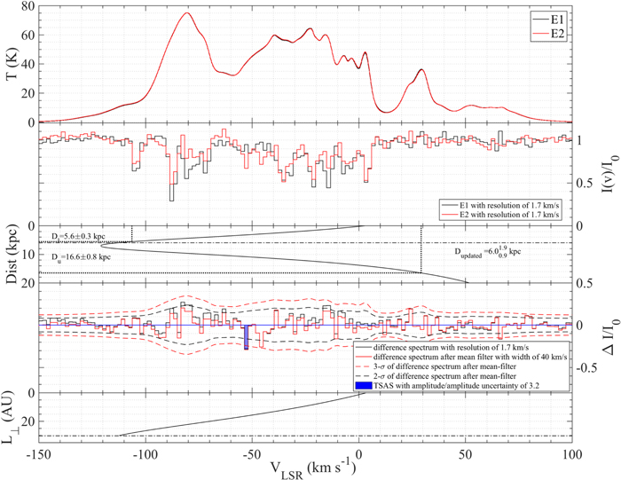
Figure 1. Spectra for PSR B1557−50. First panel: H i emission scaled to match GASS in the direction of the pulsar with a velocity resolution of 0.1 km s−1. Second panel: velocity-binned H I absorption spectra taken at E1 (black) and E2 (red) with a channel width of ∼1.7 km s−1. I(v)/I0 is as defined in Equation (2). Third panel: distance vs. radial velocity curve, calculated from Mróz et al. (2019) using the best-fit linear model with R0 = 8.09 kpc, Θ0 = 233.6 km s−1. Fourth panel: velocity-binned difference H i absorption profiles (![${\rm{\Delta }}I(v)/{I}_{0}={[I(v)/{I}_{0}]}_{{\rm{E}}2}-{[I(v)/{I}_{0}]}_{{\rm{E}}1}$](https://content.cld.iop.org/journals/2041-8205/911/1/L13/revision3/apjlabef6eieqn1.gif) ) with a channel width of 1.7 km s−1, before (black) and after (red) mean-filtering. Red and black dashed lines represent ±2σ and 3σ noise envelopes where the contribution from H i emission has been taken into account. The blue channel represents the TSAS we have identified with an S/N of 3.2. The blue horizontal line represents 0 difference. Fifth panel: spatial scale as a function of velocity. The dashed–dotted line represents the maximum spatial scale corresponding to the transverse distance traveled by the pulsar between the two epochs.
) with a channel width of 1.7 km s−1, before (black) and after (red) mean-filtering. Red and black dashed lines represent ±2σ and 3σ noise envelopes where the contribution from H i emission has been taken into account. The blue channel represents the TSAS we have identified with an S/N of 3.2. The blue horizontal line represents 0 difference. Fifth panel: spatial scale as a function of velocity. The dashed–dotted line represents the maximum spatial scale corresponding to the transverse distance traveled by the pulsar between the two epochs.
Download figure:
Standard image High-resolution imageBelow the spectra, we display the distance versus radial velocity curve, which was derived for the Galactic coordinates of PSR B1557−50 (l = 330690, b = 1
631) using a linear rotation curve (Mróz et al. 2019). A detailed description of the derivation is given in Appendix A. The lower distance limit Dl
= 5.6 ± 0.3 kpc for PSR B1557−50 is set by the velocity center of the most distant absorption feature. The upper distance limit Du
= 16.6 ± 0.8 kpc is given by the distance of the nearest significant emission component (brightness temperature above 35 K; Weisberg et al. 1979) not seen in absorption. We adopted the method described in Verbiest et al. (2012) to translate these lower and upper limits into actual distance using a likelihood analysis. The updated pulsar distance Dupdated is
 kpc. This is lower than the distance from the Australia Telescope National Facility (ATNF) pulsar catalog
  kpc, which was estimated by Verbiest et al. (2012) based on H i distance limits from Johnston et al. (2001) with a flat rotation curve (Fich et al. 1989), while higher than the distance determined from recent electron density models, which give DDM = 5.1 kpc (Yao et al. 2017).
3. Spectral Analysis, Line Profile Variations, and TSAS Properties
3.1. Spectral Analysis
We largely followed the method of Murray et al. (2018) to estimate the physical properties of each H i component, assuming that CNM can be seen in both the optical depth spectrum and the H i emission profile, while the WNM can only be seen in the emission profile. All CNM and WNM components were obtained through Gaussian decomposition (Heiles & Troland 2003a). A detailed description of the spectral decomposition and spin temperature calculation is given in Appendix B.
The derived spin temperatures for each CNM component in both epochs are listed in Table 1. Most of the CNM clouds from the two observations have spin temperatures in the range 10–260 K, which is consistent with previous observed CNM clouds (Heiles & Troland 2003b).
Table 1. Fitted Parameters of CNM Components from Gaussian Decomposition
| Epoch | τ0 | v0 | Δv0 | Ts | N(H I)abs |
|---|---|---|---|---|---|
| (name) | (km s−1) | (km s−1) | (K) | (1020 cm−2) | |
| E1 (2019.42) | 0.9 ± 0.1 | −106.18 ± 0.09 | 1.6 ± 0.2 | 11.5 ± 3.1 | 0.3 ± 0.1 |
| 3.3 ± 0.1 | −88.25 ± 0.02 | 1.49 ± 0.06 | 45.7 ± 3.2 | 4.4 ± 0.4 | |
| 1.0 ± 0.1 | −81.45 ± 0.08 | 0.9 ± 0.2 | 8.1 ± 4.9 | 0.1 ± 0.1 | |
| 0.35 ± 0.06 | −79.6 ± 0.8 | 8.4 ± 2.2 | 203.7 ± 24.5 | 12 ± 4.1 | |
| 0.5 ± 0.1 | −72.8 ± 0.3 | 2.6 ± 0.7 | 97.0 ± 7.3 | 2.2 ± 0.8 | |
| 0.67 ± 0.05 | −35.7 ± 0.2 | 5.9 ± 0.6 | 105.6 ± 4.7 | 8.3 ± 1.1 | |
| 0.79 ± 0.07 | −22.7 ± 0.2 | 3.5 ± 0.4 | 103.7 ± 3.8 | 5.7 ± 0.8 | |
| 0.83 ± 0.07 | −15.9 ± 0.2 | 3.3 ± 0.4 | 96.2 ± 4.0 | 5.3 ± 0.8 | |
| 0.5 ± 0.05 | −6.6 ± 0.3 | 6.2 ± 0.8 | 98.7 ± 5.7 | 6.2 ± 1.1 | |
| 0.79 ± 0.08 | 2.0 ± 0.1 | 2.8 ± 0.3 | 137.7 ± 9.1 | 6.0 ± 1.0 | |
| E2 (2019.78) | 0.5 ± 0.07 | −105.3 ± 0.2 | 2.4 ± 0.4 | 10.3 ± 2.5 | 0.25 ± 0.08 |
| 1.1 ± 0.1 | −88.61 ± 0.06 | 1.4 ± 0.1 | 16.7 ± 11.5 | 0.6 ± 0.4 | |
| 0.25 ± 0.04 | −78.1 ± 0.7 | 7.4 ± 1.8 | 201.8 ± 37.7 | 7.3 ± 2.6 | |
| 0.4 ± 0.1 | −72.5 ± 0.1 | 1.2 ± 0.4 | 17.6 ± 7.7 | 0.2 ± 0.1 | |
| 0.37 ± 0.06 | −53.99 ± 0.3 | 3.7 ± 0.7 | 75.5 ± 13.6 | 2.0 ± 0.7 | |
| 0.32 ± 0.05 | −46.6 ± 0.4 | 4.7 ± 1.1 | 151.6 ± 10.5 | 4.6 ± 1.3 | |
| 0.5 ± 0.1 | −37.3 ± 0.2 | 2.1 ± 0.6 | 14 ± 7.9 | 0.3 ± 0.2 | |
| 0.38 ± 0.06 | −34.8 ± 0.7 | 8.3 ± 1.3 | 157.4 ± 10.2 | 9.8 ± 2.3 | |
| 0.58 ± 0.06 | −22.5 ± 0.2 | 4.3 ± 0.5 | 86.9 ± 14.5 | 4.3 ± 1.0 | |
| 0.43 ± 0.06 | −15.0 ± 0.2 | 3.2 ± 0.6 | 131.7 ± 7.0 | 3.6 ± 0.9 | |
| 0.35 ± 0.04 | −5.8 ± 0.5 | 7.1 ± 1.2 | 99.5 ± 19.8 | 5.0 ± 1.4 | |
| 0.68 ± 0.07 | 2.3 ± 0.2 | 3.0 ± 0.4 | 102.1 ± 20.7 | 4.1 ± 1.1 | |
Note. Columns (1): observing epoch. Columns (2)–(4): Gaussian parameters fit to the opacity profile (Equation (B1)). Column (4): H i spin temperature. Column (5): H i column density of absorption component calculated by N(HI)abs = C0∫τ Ts dv = 1.064 · C0 · τ0 · Δv0 · Ts , where C0 = 1.823 × 1018 cm−2/(km s−1 K) (Murray et al. 2018).
Download table as: ASCIITypeset image
3.2. Line Profile Variations and TSAS Properties
In order to evaluate H i absorption profile variations between the two epochs, we first define a difference H i absorption profile ![${\rm{\Delta }}I(v)/{I}_{0}={[I(v)/{I}_{0}]}_{{\rm{E}}2}-{[I(v)/{I}_{0}]}_{{\rm{E}}1}$](https://content.cld.iop.org/journals/2041-8205/911/1/L13/revision3/apjlabef6eieqn4.gif) . Here it is crucial to account accurately for the noise profile, where the H i emission tends to dominate over system temperature in this band (Weisberg et al. 2008). We thus added the H i antenna temperature, in the velocity range where it can be measured, to the system temperature. The resultant noise profile is given by
. Here it is crucial to account accurately for the noise profile, where the H i emission tends to dominate over system temperature in this band (Weisberg et al. 2008). We thus added the H i antenna temperature, in the velocity range where it can be measured, to the system temperature. The resultant noise profile is given by ![${\sigma }_{{\rm{\Delta }}I/{I}_{0}}(v)={\sigma }_{{\rm{\Delta }}I/{I}_{0},\mathrm{off}-\mathrm{line}}\times [{T}_{{\rm{H}}{\rm\small{I}}}(v)+{T}_{\mathrm{sys},\mathrm{off}-\mathrm{line}}]/{T}_{\mathrm{sys},\mathrm{off}-\mathrm{line}}$](https://content.cld.iop.org/journals/2041-8205/911/1/L13/revision3/apjlabef6eieqn5.gif) , where Tsys,off‐line is the system temperature for off-line channels, TH I(v) is the antenna temperature of H i at velocity v, and
, where Tsys,off‐line is the system temperature for off-line channels, TH I(v) is the antenna temperature of H i at velocity v, and  is the absorption spectrum standard deviation of off-line channels (Weisberg et al. 2008). In order to mitigate the effect of residual baseline ripples on ΔI(v)/I0, we constructed a boxcar mean-filter with a width of 40 km s−1, based on the width of the residual ripples, and subtracted it from the difference spectrum. We propagated the uncertainties associated with the mean-filter to determine the final noise envelope of the difference spectrum after mean-filtering.
We adopted a two-stage approach to Gaussian fitting of the mean-filtered difference spectrum. First, we used a Markov Chain Monte Carlo (MCMC) method to obtain an initial list of TSAS candidates. The MCMC sampling was performed using the emcee package (Foreman-Mackey et al. 2013), with the range of Gaussian parameters for the prior obtained from the properties of the absorption components at the two epochs. We then treated all components with local minima as constrained from MCMC as TSAS candidates. We next performed a traditional χ2 fitting on those candidates using the LMFIT package (Newville et al. 2019), with initial guesses for the Gaussian parameters drawn from the MCMC output. We define the signal-to-noise ratio (S/N) of the component as the ratio of the fitted amplitude to the 1σ amplitude uncertainty output by LMFIT (where the appropriate noise spectrum has been used as the uncertainty input). This 1σ amplitude uncertainty is estimated from the square root of the diagonal elements of the covariance matrix. By this definition, there is one tentative TSAS showing a marginal detection with an S/N of 3.2 at a velocity of ∼−54 km s−1, shown in the fourth panel of Figure 1. Note that while the spectrum is binned in velocity to a channel width of 1.7 km s−1 to illustrate the TSAS clearly, the fitting was performed on the unbinned data.
Compared to previous TSAS detections toward this pulsar (Deshpande et al. 1992; Johnston et al. 2003), we have a much higher velocity resolution of ∼0.1 km s−1, reduced artifacts on the difference spectrum, and an estimated distance for each channel, enabling us to obtain TSAS detection results with definitive spatial scales. The spatial scale L⊥(v) was calculated using  , where PMTOT is pulsar total proper motion of 14 mas yr−1 from the ATNF pulsar catalog (Manchester et al. 2005), and Δt is the time baseline. The characteristic scale of the tentative TSAS that we probe is 17 au, which is much smaller than the TSAS previously detected toward PSR B1557−50 (∼1000 au at the velocity of −110 km s−1 assuming the pulsar velocity of 400 km s−1 and the component distance of 6.4 kpc) with a time baseline of 20 yr. This is due to the short time interval between the two observations.
The observed properties of the single tentatively detected TSAS component are summarized in Table 2. We assume that the TSAS has the same spin temperature as its host CNM cloud (75.5 ± 13.6 K). The derived value of the H i column density of the tentative TSAS is (7 ± 3) × 1019 cm−2, consistent with the column densities of previous TSAS studies, which range from 1019 to 1021 cm−2 (Stanimirović & Zweibel 2018). In total, the tentative TSAS feature contributes ∼34% to the total H i column density of its host CNM cloud.
Table 2. Tentative TSAS Properties
| Center Velocity | L⊥ | Dist | Δv0 | Δτ | Ts | N(H I)TSAS | n(H I)TSAS | P/k |

|
σtur/
|
σth/
|
|---|---|---|---|---|---|---|---|---|---|---|---|
| (km s−1) | (au) | (kpc) | (km s−1) | ( K) | (1020 cm−2) | (104 cm−3) | (106 cm−3 K) | (1020 cm−2) | (km s−1) | (km s−1) | |
| −53.5 ± 0.2 | 17 | 3.3 ± 0.3 | 1.3 ± 0.5 | 0.35 ± 0.11 | 75.5 ± 13.6 | 0.7 ± 0.3 | 26.6 ± 13.7 | 20.7 ± 12.5 | 0.03 | 0.2 ± 0.1/0.5 | 0.8 ± 0.1/0.3 |
Note. Column (1): TSAS central velocity. Column (2): TSAS spatial scale. Column (3): TSAS distance. Column (4): FWHM of TSAS. Column (5): maximum absolute value of optical depth variations. Column (6): spin temperature. Column (7): TSAS H i column density. It is calculated by N(H I)TSAS = 1.064 · C0 · ∣Δτ∣ · Δv0 · Ts . Column (8): TSAS H i volume density. Column (9): thermal pressure. Column (10): the minimum column density calculated when the dynamical time is larger than the cooling time. Column (11): the one-dimensional turbulent velocity/the one-dimensional turbulent velocity when the TSAS spin temperature is 10 K. Column (12): the one-dimensional thermal velocity/the one-dimensional thermal velocity when the TSAS spin temperature is 10 K.
Download table as: ASCIITypeset image
4. Discussion
If the tentative TSAS is a spherical cloud with diameter of L⊥, the derived H i volume density and thermal pressure are larger than ∼104 cm−3 and ∼ 106 K cm−3, respectively. These values are consistent with previous TSAS studies (assuming similar geometry), with TSAS showing densities and thermal pressures two to three orders of magnitude larger than typical ISM values (Heiles 1997; Stanimirović et al. 2010; Stanimirović & Zweibel 2018).
When the dynamical time tdyn is larger than the cooling time tcool, clouds may reach a thermal equilibrium, even if they are overpressured. The column density  for a cloud at the balance of cooling and expanding can be calculated. As estimated by Stanimirović & Zweibel (2018),
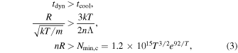
where R is the size of the cloud, T is the kinetic temperature, and Λ is the radiative loss function assuming the Cii fine structure line is the main source of cooling, with a carbon depletion factor of 0.35. Clouds with a column density larger than  would cool radiatively faster than they expand and reach thermal equilibrium. We use the H i spin temperature as an approximation of the kinetic temperature (Lauroesch & Meyer 2003) to estimate
  . We found that our tentative TSAS component has N(H I)TSAS significantly larger than
  , suggesting that it may be overpressured and in thermal equilibrium with the ambient ISM.
To alleviate the problem of overpressurization, Heiles (1997) proposed a model in which TSAS represents discrete features in the shape of cylinders and disks that are homogeneously and isotropically distributed within CNM clouds. The volume density of TSAS depends both on the spatial scale across the LOS, L⊥, and the path length along the LOS L∥. Following Heiles (1997), we define the geometric elongation factor  = L∥/L⊥ and use the standard CNM thermal pressure of 4000 cm−3 K. Based on our measured spin temperature and column density, the elongation factor
  required for our tentative TSAS to match the CNM pressure is ∼5000. Such extremely filamentary structure is out of the range predicted by Heiles (1997), who found
  larger than 1 and less than 10. This is a result of the large variation of optical depth and the small spatial scale of the tentative TSAS that we detected.
Hennebelle & Audit (2007) found that CNM clouds can be generated from thermally unstable regions in colliding WNM flows based on simulations with resolutions of 400 and 4000 au (larger than the typical spatial scales of observed TSAS). The supersonic collisions of CNM clouds form transient shocked regions with large temperature variations at the boundaries, showing similar properties to TSAS. Such temperature variations could induce line width and optical depth variations in the observed H i absorption spectrum. From Figure 1 and Table 1 it can be seen that, in addition to apparent optical depth variations, the spin temperatures and line widths of the CNM components detected in this work do exhibit differences between the two epochs. While much of this variation lies below strict 3σ limits, it may still be indicative of the variations predicted by colliding flows models, possibly suggesting that our tentative TSAS cloud could have formed from such colliding WNM flows. However, better evidence of variability in the data, together with detailed descriptions of the properties of TSAS from higher-resolution simulations (<100 au), are needed to make firm quantitative comparisons.
Finally, compressible turbulence can generate density fluctuations and may even be able to confine an overpressured structure. Stanimirović & Zweibel (2018) estimate that in order to confine TSAS-like structures that are overpressured by a factor of ∼100, the turbulent velocity must be at least 10 times the rms thermal velocity (see also McKee & Zweibel 1992). Following Rybarczyk et al. (2020), we estimate the one-dimensional turbulent velocity σtur for the tentative TSAS components by assuming that the nonthermal component of the velocity dispersion is entirely accounted for by turbulent motions such that

where  is the mass of hydrogen atom, σth is the one-dimensional rms thermal velocity, and the spin temperature Ts
is assumed to be a good approximation of the kinetic temperature for the CNM. The turbulent velocity is far too small to confine the tentative TSAS, with σtur = 0.2 km s−1 and σth = 0.8 km s−1 (see also Table 2). If we instead adopt a minimum possible value of 10 K for the spin temperature, we can calculate a lower limit for σth and the corresponding upper limit for σtur (as denoted by
is the mass of hydrogen atom, σth is the one-dimensional rms thermal velocity, and the spin temperature Ts
is assumed to be a good approximation of the kinetic temperature for the CNM. The turbulent velocity is far too small to confine the tentative TSAS, with σtur = 0.2 km s−1 and σth = 0.8 km s−1 (see also Table 2). If we instead adopt a minimum possible value of 10 K for the spin temperature, we can calculate a lower limit for σth and the corresponding upper limit for σtur (as denoted by  km s−1 and
  km s−1 in Table 2). Even in this case, the turbulent velocity is still less than 10 times the rms thermal velocity. This suggests that the turbulent velocity is not sufficient to confine the tentative TSAS.
5. Conclusions
We have obtained H i absorption spectra in two epochs 0.36 yr apart toward PSR B1557−50 with the Parkes telescope. We have detected one component with marginally significant absorption variations, which probes astronomical-unit-scale atomic structure in the Milky Way. Our main results are summarized as follows:
1. One TSAS component at ∼−54 km s−1 was marginally detected with an S/N of 3.2 after carefully reducing artifacts on the difference spectrum.
2. The characteristic plane-of-sky spatial scale of the TSAS component is 17 au, with an inferred volume density (assuming a spherical cloud) of 2.7 × 105 cm−3, and thermal pressure of 2.1 × 107 cm−3 K, suggesting that the TSAS is overdense and overpressured by two to three orders of magnitude.
3. The inferred overpressured TSAS has sufficiently high column density to be in thermal equilibrium with the ambient ISM, while still being overpressured.
4. The elongation factor of the TSAS cloud would need to be ∼5000 in order for it to be in pressure equilibrium with a canonical CNM. This is much larger than expected from disks or cylinders (Heiles 1997), and than the aspect ratio of observed ISM filaments.
5. In addition to optical depth variations, there is some evidence of line width and temperature variations in the CNM components observed at the two epochs. This may hint at a possible formation mechanism involving WNM collisions.
6. We consider a scenario in which the TSAS represents the tail-end of a turbulent cascade, and find that the turbulent line width would be insufficient to confine such an overpressured cloud.
Further monitoring of this pulsar, as well as other pulsars with previous H i absorption measurements using single-dish telescopes (e.g., Parkes, FAST), would enable us to detect a larger population of TSAS, and with sensitivity to a wide range of spatial scales, which may be critical in better probing the role of turbulence in TSAS formation. More generally, future high-resolution, interferometric observations (e.g., with the VLA, ALMA) of atomic and molecular lines (e.g., H i, CO, C i, C ii, SiO) toward TSAS associated with a larger range of spin temperature estimates are necessary to better constrain TSAS cooling and heating mechanisms, and shed crucial light onto TSAS formation.
This work is supported by National Natural Science Foundation of China (NSFC) program Nos. 11988101, 11725313, 11690024, by the CAS International Partnership Program No. 114-A11KYSB20160008, and the National Key R&D Program of China (No. 2017YFA0402600). Cultivation Project for FAST Scientific Payoff and Research Achievement of CAMS-CAS. J.R.D. is the recipient of an Australian Research Council (ARC) DECRA Fellowship (project number DE170101086). We are grateful to Lawrence Toomey for supporting the data transfer and processing. We thank CSIRO computing resources for data storage and processing. We express our thanks to Claire Murray for Gaussian decomposition and fitting discussions; Shi Dai, Weiwei Zhu, Lei Zhang, Chenchen Miao for dispersion measurement (DM) discussions; Jumei Yao for DM-based distance discussions; James Green for his help in observation arrangement at Parkes; Zhichen Pan and Yi Feng for supporting the data transfer; Lei Qian for the turbulent velocity discussion; Zheng Zheng for baseline removal discussion; Chaowei Tsai and Guodong Li for the MCMC discussion.
Appendix A: The Distance–Radial Velocity Curve Derivation
Mróz et al. (2019) used a sample of 773 Classical Cepheids with precise distances based on mid-infrared period–luminosity relations coupled with proper motions and radial velocities from Gaia to construct an accurate rotation curve of the Milky Way up to a distance of ∼20 kpc from the Galactic center. They found linear rotation curves describe that data much better than a simple constant rotation curve and are more consistent with previous observations than the universal rotation curve.
For an object in circular rotation about the galactic center at radius R with circular velocity ω, by adopting the best-fit linear model from Mróz et al. (2019)

where ω0 is the angular velocity of the Sun’s rotation around the Galaxy, the radial velocity with respect to the LSR is given by

where R0 and VΠ represent the galactocentric distance of the Sun and the net outward motion of the LSR with respect to the Galactic object that is 4.2 km s−1, respectively. Similar to Weisberg et al. (2008), we add and subtract velocities of 7 km s−1 to Vr to estimate the uncertainties in distance limits due to streaming and random gas motions in the Galaxy.
With  , the distance–radial velocity relation can be derived:

Appendix B: Gaussian Decomposition and Spin Temperature Estimation
We largely followed the method described in Murray et al. (2018) to estimate the spin temperature. This method was developed based on the strategy first proposed by Heiles & Troland (2003a). They used a least-squares fitting method to fit Gaussian components to both H i absorption and emission spectra in order to estimate the physical properties of the H i clouds. Compared to the traditional fitting method described in Heiles & Troland (2003a), Murray et al. (2018) adopted an autonomous Gaussian decomposition algorithm (Gausspy), which implements a derivative spectroscopy technique to use supervised machine learning to estimate the number of Gaussian features and their properties. We used an upgraded, fully autonomous, Gaussian decomposition algorithm via its open-source Python implementation (GaussPy+; Riener et al. 2019) to make initial guesses for Gaussian components toward PSR B1557−50 and applied a least-squares fitting to refine the results.
According to Heiles & Troland (2003a), the optical depth spectrum τ(v) along the LOS with a set of N Gaussian components can be written as

where τ0,n , v0,n , and Δvn are the the peak optical depth, central velocity, and FWHM of the nth component.
The optical depth spectrum is only contributed by the CNM, while the brightness temperature-calibrated Toff(v) consists of both the CNM and the WNM,

where TB,CNM is the H i emission contributed by the CNM and TB,WNM(v) is the H i emission contributed by the WNM. The H i emission contributed by N CNM components can be written as

where m represents M absorption clouds lying in front of the nth cloud, and Ts,n
represents the spin temperature for the nth component. For the H i emission contributed by the WNM TB,WNM(v), can be considered as a set of K Gaussian functions. For each kth component, there is a fraction  of the WNM is located in front of all CNM components.

where v0,k , Δvk , and T0,k represent the central velocity, FWHM, and peak brightness temperature for the kth emission component.
Based on the method described in Murray et al. (2018), spin temperatures can be estimated with the following steps:
- 1.Decompose Gaussian components for τ(v) with GaussPy+ to make initial guesses. Following the method described in Riener et al. (2019), we applied the algorithm on the optical depth profiles constructed from absorption lines of PSR B1557−50. We chose the two-phase smoothing parameters α1 = 2.58 and α2 = 5.14, and a minimum S/N of 5 for signal peaks in the data to decompose the optical depth profiles.
- 2.Fit N components to τ(v) via least-squares fitting using the LMFIT package (Newville et al. 2019). The components were selected from step (1), restricted to those with line widths less than 20 km s−1, and which are well separated. The mean velocities, widths, and amplitudes are allowed to vary by ±20% with respect to the GaussPy+ fit parameters. τ(v) was decomposed into 10 and 12 components for E1 and E2, respectively, which are shown as blue lines in the third panels of Figure 2.
- 3.Fit the N components from τ(v) to
 via least-squares fitting. The mean velocities and widths are allowed to vary by ±10%. Ts
are constrained to between , to produce physically realistic spin temperatures.
via least-squares fitting. The mean velocities and widths are allowed to vary by ±10%. Ts
are constrained to between , to produce physically realistic spin temperatures. - 4.Subtract the best-fit model in step (3) from to produce a residual emission spectrum, which contains only WNM components not previously modeled.
- 5.Fit K components to the residual emission spectrum from (4) with GaussPy+, using α1 = 2.58, α2 = 5.14, and S/N = 740.
- 6.Use least-squares fitting to fit with N + K Gaussian components from steps (2) and (5). The mean velocities and widths are allowed to vary by 10% with respect to the previously fitted values. The amplitudes are constrained so that . The final estimation of Ts
for the N absorption components and the Gaussian parameters of the K emission-only components is computed based on Equations (B2)–(B4).




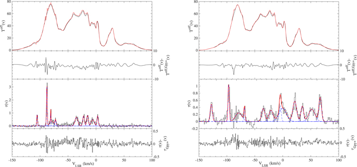
Figure 2. For two epoch observations (left: E1, right: E2). The brightness temperature-calibrated H i emission spectrum  and the fitting spectra
  in the red line (the top panels), the fitting residual of the H i emission spectrum (the second panels), the optical depth profile τ(v), the decomposed Gaussian components in the dashed blue lines, and the fitting optical depth profile τGpy+(v) in the red line (the third panels), and the fitting residual of the optical depth profile (the bottom panels). The spectra were binned in velocity to a channel width of 0.6 km s−1.
Download figure:
Standard image High-resolution imageWhen the absorption components overlap in velocity significantly, the order of each component will affect TB,CNM(v) (Heiles & Troland 2003a; Stanimirović et al. 2010; Murray et al. 2018). There are a maximum of N
! different orderings of components along the LOS. In the case of our optical depth profiles, the components are well separated, so we did not need to consider the ordering phenomenon during fitting. Previous studies have indicated that the values of  have significant effect on the derived spin temperature (Heiles & Troland 2003a; Stanimirović et al. 2010; Murray et al. 2018). We followed previous analyses to estimate the spin temperature by assigning value of 0.0, 0.5, or 1.0 to
  . Therefore, there are three possible cases for the final fit of
  from our data.
The final spin temperatures are calculated by estimating the weighted mean and standard deviation over the three iterations following Heiles & Troland (2003a). For the spectra observed in E1 and E2, we fit 10 (N = 10) and 12 (N = 12) absorption components and 27 (K = 27) and 26 (K = 26) emission-only components, respectively. Figure 2 illustrates the Gaussian decomposition and fitting of the H i emission and optical depth profiles for E1 and E2, respectively. The main results of the CNM decomposition are shown in Table 1.