Abstract
Multimessenger observations of coalescing binary neutron stars (BNSs) using gravitational-wave (GW) and electromagnetic- (EM) wave signals are a direct probe of the expansion history of the Universe and carry the potential to shed light on the disparity between low- and high-redshift measurements of the Hubble constant H0. To measure the value of H0 with such observations requires pristine inference of the luminosity distance and the true source redshift with minimal impact from systematics. In this analysis, we carry out joint inference on mock GW signals and their EM afterglows from BNS coalescences and find that the inclination angle inferred from the afterglow light curve and apparent superluminal motion can be precise but need not be accurate and is subject to a systematic uncertainty that could be as large as 1.5σ. This produces a disparity between the EM and GW inferred inclination angles, which if not carefully treated when combining observations can bias the inferred value of H0. We also find that already small misalignments of 3°–6° between the inherent system inclinations for the GW and EM emission can bias the inference by  if not taken into account. As multimessenger BNS observations are rare, we must make the most out of a small number of events and harness the increased precision while avoiding a reduced accuracy. We demonstrate how to mitigate these potential sources of bias by jointly inferring the mismatch between the GW- and EM-based inclination angles and H0.
Original content from this work may be used under the terms of the Creative Commons Attribution 4.0 licence. Any further distribution of this work must maintain attribution to the author(s) and the title of the work, journal citation and DOI.
1. Introduction
The bright sirens method for measuring the Hubble flow in the local Universe accessible to gravitational-wave (GW) detectors was proposed by B. F. Schutz (1986) based on the robust prediction by general relativity (GR) of the luminosity and time evolution of a binary neutron star (BNS) coalescence. It has been validated at the single-event level by the multimessenger observation of GW170817, which provided luminosity distance and redshift information independently (e.g., B. P. Abbott et al. 2017a) and produced a ∼15% measurement of the Hubble parameter H0; see B. P. Abbott et al. (2017b). This measurement of the Hubble parameter is further improved to a ∼7% measurement by including the observation of a radio jet and improved peculiar velocity (see B. P. Abbott et al. 2017b; K. Hotokezaka et al. 2019; S. Mukherjee et al. 2021). Though such measurements are theoretically robust, in practice, multiple astrophysical uncertainties such as inclination angle (S. Nissanke et al. 2010), peculiar velocity (T. M. Davis et al. 2019; C. Nicolaou et al. 2020; S. Mukherjee et al. 2021; H. Nimonkar & S. Mukherjee 2023), waveform uncertainty (N. Kunert et al. 2024), nonstationary noise (S. Mozzon et al. 2022), etc. can obscure the inference of H0 if not taken into account correctly. To accurately infer the value of the Hubble constant from GW data and shed light on the ongoing tension on the true value of the Hubble constant (see E. Abdalla et al. 2022 for a review), it is important to mitigate the influence of any possible systematic due to astrophysical and instrument uncertainties.
In order to mitigate these additional uncertainties, combining GW and electromagnetic (EM) observations can be beneficial. For a BNS or black hole–neutron star (BHNS) merger, the remnant, if matter is still present, is expected to source a highly relativistic, collimated matter outflow (jet) from its poles, which produces a short gamma-ray burst (GRB;  ) and a long-lived transient spanning all wavelengths (
 ) called the afterglow (see E. Berger 2014; B. P. Abbott et al. 2017a; E. Nakar & T. Piran 2021). Besides allowing for the identification of a host galaxy, and through that a redshift, the EM counterpart can also mitigate a degeneracy between the luminosity distance (dL
) and the system orientation in the GW analysis, which limits the precision of the dL
measurement (e.g., S. Nissanke et al. 2010; B. F. Schutz 2011).
) called the afterglow (see E. Berger 2014; B. P. Abbott et al. 2017a; E. Nakar & T. Piran 2021). Besides allowing for the identification of a host galaxy, and through that a redshift, the EM counterpart can also mitigate a degeneracy between the luminosity distance (dL
) and the system orientation in the GW analysis, which limits the precision of the dL
measurement (e.g., S. Nissanke et al. 2010; B. F. Schutz 2011).
The angle between the observer line of sight  and the orbital angular momentum axis
  (see Figure 1) is generally referred to as the system inclination, θJN. Since the jet comes from a polar outflow of the remnant, θJN is expected to be correlated with the jet inclination.
5
While (non)observation of the prompt γ-ray emission can provide a weak (lower) upper bound on the viewing angle due to its highly collimated nature, the light curve of the afterglow, which is also detectable further off-axis, is more sensitive to the viewing angle θvi (which is defined as the angle between the jet's direction of propagation
(see Figure 1) is generally referred to as the system inclination, θJN. Since the jet comes from a polar outflow of the remnant, θJN is expected to be correlated with the jet inclination.
5
While (non)observation of the prompt γ-ray emission can provide a weak (lower) upper bound on the viewing angle due to its highly collimated nature, the light curve of the afterglow, which is also detectable further off-axis, is more sensitive to the viewing angle θvi (which is defined as the angle between the jet's direction of propagation  and the observer’s line of sight
  ; see Figure 1). In particular, the initial rising slope of the light curve (for bright signals) and the jet break contain orientation information and allow extraction of the viewing angle (e.g., E. Nakar & T. Piran 2021; G. Ryan et al. 2024). The constraint from the light curve is actually on a combination of the viewing angle and opening angle of the jet, and this degeneracy curtails the precision of the measurement (G. Ryan et al. 2020; K. Takahashi & K. Ioka 2020; E. Nakar & T. Piran 2021). A possible way to break the degeneracy in the light-curve data is through astrometry performed on the radio image of the afterglow, which can reveal a lateral apparent superluminal motion of the afterglow centroid that is highly sensitive to the viewing angle
6
and thus lead to a 10%-level measurement of the viewing angle; see, e.g., K. P. Mooley et al. (2018). Such a constraint for the viewing angle, combined with assumptions about its correlation with the system inclination, can limit or break the degeneracy between θJN and dL
and improve the precision of the dL
–H0 measurement by a factor of 2 (S. Nissanke et al. 2010; H.-Y. Chen et al. 2019). However, by including EM data, the clear dependence of the inferred dL
on GR alone is lost, and one has to make sure that the additional precision at the single-event level is not accompanied by a reduced accuracy in the inference.
; see Figure 1). In particular, the initial rising slope of the light curve (for bright signals) and the jet break contain orientation information and allow extraction of the viewing angle (e.g., E. Nakar & T. Piran 2021; G. Ryan et al. 2024). The constraint from the light curve is actually on a combination of the viewing angle and opening angle of the jet, and this degeneracy curtails the precision of the measurement (G. Ryan et al. 2020; K. Takahashi & K. Ioka 2020; E. Nakar & T. Piran 2021). A possible way to break the degeneracy in the light-curve data is through astrometry performed on the radio image of the afterglow, which can reveal a lateral apparent superluminal motion of the afterglow centroid that is highly sensitive to the viewing angle
6
and thus lead to a 10%-level measurement of the viewing angle; see, e.g., K. P. Mooley et al. (2018). Such a constraint for the viewing angle, combined with assumptions about its correlation with the system inclination, can limit or break the degeneracy between θJN and dL
and improve the precision of the dL
–H0 measurement by a factor of 2 (S. Nissanke et al. 2010; H.-Y. Chen et al. 2019). However, by including EM data, the clear dependence of the inferred dL
on GR alone is lost, and one has to make sure that the additional precision at the single-event level is not accompanied by a reduced accuracy in the inference.

Figure 1. Sketch for the definition of the system inclination θJN during the inspiral/merger on the left and for the definition of the jet viewing angle θvi and misalignment angle θm for the postmerger remnant. The line of sight for the observer is indicated with the vector  .
.
Download figure:
Standard image High-resolution imageIn particular, the interpretation of the photometry and astrometry data for the jet afterglow and its connection to the properties of the merging compact binary system requires the assumption of a model that describes the emission from the jet afterglow. However, the emission model for the afterglow that is fit to the EM data to constrain θvi is strongly dependent on the assumed jet structure and geometry. Understanding the latter based on the properties of the merging binary, unfortunately, is presently not feasible due to the computational challenges involved in the physical processes at vastly different scales that govern the merger and subsequent remnant evolution with jet formation (L. Combi & D. M. Siegel 2023; E. R. Most & E. Quataert 2023; K. Kiuchi et al. 2024 for BNS and E. R. Most et al. 2021; K. Hayashi et al. 2022 for BHNS) and then jet propagation (R. Fernández et al. 2019; A. Kathirgamaraju et al. 2019) and nonthermal emission (e.g., J. Granot & R. Sari 2002). Thus, one has to assume a particular model for the jet structure to fit the light curve and centroid motion, which cannot be constrained by knowledge about the inspiraling binary from the GW data. We refer to the systematic uncertainty in the inference of H0, if the inference of θvi is incorrect due to a theoretical modeling choice, as model bias.
Furthermore, while the GW and EM emission share the luminosity distance as a common parameter, it is necessary to specify a relation between the viewing angle for the jet and the system inclination for the inspiraling binary. It is often assumed that the jet axis is aligned with the total angular momentum of the postmerger system and that this in turn does not deviate much from the orbital angular momentum of the merging system—see, e.g., B. P. Abbott et al. (2017c), H.-Y. Chen et al. (2019), and A. Farah et al. (2020)—which allows for a direct identification of the two parameters when the posteriors on θJN and θvi are combined. However, there is presently no theoretical framework for confirming this assumption, and in general, a misalignment of  between the three axes might be present due to remnant properties (e.g., N. Stone et al. 2013; K. Hayashi et al. 2022; Y. Li et al. 2023) or collimation in an anisotropic medium (e.g., H. Nagakura et al. 2014). We define the line-of-sight misalignment angle as θm = θJN − θvi
7
(see Figure 1) and refer to systematic deviations in H0 due to an intrinsic mismatch between the jet angle and inclination angle (
between the three axes might be present due to remnant properties (e.g., N. Stone et al. 2013; K. Hayashi et al. 2022; Y. Li et al. 2023) or collimation in an anisotropic medium (e.g., H. Nagakura et al. 2014). We define the line-of-sight misalignment angle as θm = θJN − θvi
7
(see Figure 1) and refer to systematic deviations in H0 due to an intrinsic mismatch between the jet angle and inclination angle ( ) as misalignment bias.
The effect of model and misalignment biases is similar in the sense that both will shift the EM posterior with respect to the GW posterior and, consequently, the region of joint posterior support, as shown in Figure 2, and a failure to take this into account in the joint inference will bias the combined posterior for dL . In particular, Figure 2 shows that a positive/negative misalignment angle, which is equivalent to an under-/overestimation of the viewing angle in the model bias scenario, will bias the posterior support toward larger/smaller dL due to the anticorrelation of the GW posterior in the dL –θJN plane.

Figure 2. The GW (heat map and black contours) and EM (red contours) posteriors in the dL
–θvi plane for injected/true parameters θJN = 30° and dL
= 21.56 Mpc (marked in white). The dashed and solid contours indicate the 1σ and 2σ highest posterior density credible regions. The yellow and magenta contours show two EM posteriors with a positive or negative angular shift of 57 between the jet angle and system inclination (the injected/true θvi is indicated with stars).
Download figure:
Standard image High-resolution imagePreviously, the presence of a model bias has been studied in great detail for the EM counterpart of GW170817 (K. P. Mooley et al. 2018; Z. Doctor 2020; E. Nakar & T. Piran 2021; G. Gianfagna et al. 2023, 2024; T. Govreen-Segal & E. Nakar 2023). While these authors study the systematic based on GW170817 and/or future similar events 8 with detailed EM modeling, the more general analysis of H.-Y. Chen (2020) uses Gaussian estimates for EM likelihoods. 9 Consequently, a systematic exploration of the model bias for systems that differ from GW170817 that employs realistic EM inference models and mock data has been missing so far.
This Letter points out that the misalignment between the jet direction inferred from EM observations and GW observations can be a potential hindrance in achieving accurate H0 at the single-event level and the ultimate bottleneck when the statistical uncertainty is negligible. By performing joint cosmological inference on a suite of realistic mock data simulations, we show that due to a positive/negative value of the misalignment angle, there can be an under-/overestimation of H0. We propose a Bayesian technique to mitigate this effect in a multimessenger analysis where light-curve, centroid motion of the jet, and GW data are used to infer the value of H0.
2. Methods
To study the impact of potential model and misalignment biases on the joint GW+EM inference, we generate a series of mock observations in the GW and EM sectors that are consistent with an equal-mass BNS assuming different system inclinations and jet viewing angles in the range 0°–80°, which allows us to combine posteriors from both sources that either have an intrinsic misalignment between the jet and orbital angular momentum axes ( ) or not.
We restrict the present analysis to BNS systems for simplicity. While BHNS systems may differ in the details of the jet launching mechanism and structure, if they launch a relativistic jet, we expect broadly similar phenomenology to a BNS: a GW inspiral with dL
–θvi degeneracy and a nonthermal EM synchrotron afterglow (see also M. Ruiz et al. 2019). While the asymmetries introduced by unequal masses or misaligned component spins have, in principle, the capacity to lead to a misaligned jet, a more complete theoretical understanding of the jet formation is required to leverage such correlations. Consequently, as a first step, we only consider equal-mass binaries in this analysis. We consider a flat Lambda cold dark matter cosmology (see H. Mo et al. 2010) with  km s−1 Mpc−1, consistent with B. P. Abbott et al. (2017b), and we fix the redshift to z(true) = 0.005, which corresponds to a luminosity distance of
  Mpc, since we will not focus on the peculiar velocity bias. This is an unrealistically small distance (for comparison, GW170817 was observed at around 40 Mpc; see B. P. Abbott et al. 2017b), and it will lead to superideal posteriors; however, we investigate the biases under such optimal conditions to clearly distinguish between statistical fluctuations (which should be strongly suppressed in the considered loud signals) from systematic deviations. We shall use a particular jet structure to generate all of the events; see Section 2.2.2 for details. Below, we outline the statistical framework that is used for the joint GW+EM inference of the Hubble parameter, as well as the methods with which we generated our mock observations in both sectors.
2.1. Bayesian Framework
From Bayes’s theorem (M. Bayes & M. Price 1763), we obtain the joint Hubble posterior through

where  is the collection of all relevant data sets from the EM and GW sectors, respectively, and
  represents the prior/model assumptions under which the inference is performed. Assuming that the measurements in the subsectors are independent and that the data only depend on the event parameters θ, the data likelihood for the joint inference model is

where  represents the prior assumptions for the analysis of the combined data. In this work, we are interested in combining posterior knowledge about the redshift z, the luminosity distance dL
, the inclination of the GW source θJN, and the viewing angle for the postmerger jet θvi to learn about H0, and both observation channels have access to different but overlapping subsets of this parameter space. As discussed in Sections 2.2.1 and 2.2.2, the respective models for the jet afterglow and the GW emission have a much higher parameter space with complex correlations; however, we shall marginalize the full posteriors to the relevant subspace θ = θEM ∪ θGW, with
represents the prior assumptions for the analysis of the combined data. In this work, we are interested in combining posterior knowledge about the redshift z, the luminosity distance dL
, the inclination of the GW source θJN, and the viewing angle for the postmerger jet θvi to learn about H0, and both observation channels have access to different but overlapping subsets of this parameter space. As discussed in Sections 2.2.1 and 2.2.2, the respective models for the jet afterglow and the GW emission have a much higher parameter space with complex correlations; however, we shall marginalize the full posteriors to the relevant subspace θ = θEM ∪ θGW, with  and
and  . In the choice of the
  prior for the joint inference, we assume the general scenario where the jet viewing angle and system inclination differ by a misalignment angle θm, whose value is determined by an a priori assumption in
  . Furthermore, there is a mismatch in the parameter range of θvi and θJN, since the reflection symmetry of the jet about the spin plane causes the scenarios θvi and
  to be indistinguishable. Thus, the GW inclination parameter will always be converted to a value compatible with θvi with
  (e.g., B. P. Abbott et al. 2017c). In the context of the inference, these are still treated as separate parameters, but we enforce this relation in the Hubble inference prior, which we shall take to be of the following form:

where the priors  and
and  are chosen to be Dirac delta distributions to account for the different parameters’ correlations. We have already introduced the misalignment angle θm as a free parameter in the prior for θvi to account for the possibility that we have a nonzero shift between θJN and θvi. In this work, we also assume that the redshift can be measured with high precision,
10
to the point that we can approximate the likelihood/posterior as a Dirac delta distribution. Inserting the prior, expressing the GW and EM data likelihoods in terms of posteriors, and integrating out all of the Dirac delta distributions result in the following reduced form for the combined data likelihood:
are chosen to be Dirac delta distributions to account for the different parameters’ correlations. We have already introduced the misalignment angle θm as a free parameter in the prior for θvi to account for the possibility that we have a nonzero shift between θJN and θvi. In this work, we also assume that the redshift can be measured with high precision,
10
to the point that we can approximate the likelihood/posterior as a Dirac delta distribution. Inserting the prior, expressing the GW and EM data likelihoods in terms of posteriors, and integrating out all of the Dirac delta distributions result in the following reduced form for the combined data likelihood:
We choose to use a uniform prior for the Hubble parameter, ![$\pi \left({H}_{0}| {\lambda }_{{H}_{0}}\right)={ \mathcal U }\left[0,200\right]$](https://content.cld.iop.org/journals/2041-8205/977/2/L45/revision1/apjlad8dd1ieqn27.gif) km s−1 Mpc−1, where
km s−1 Mpc−1, where  denotes the uniform distribution between two bounds. The priors for the λGW and λEM models that are used for the posteriors in the disjoint GW and EM analysis are specified in Section 2.2.1 and Appendix A.
2.2. Mock Data Generation
The posteriors that will be used in the framework described above are obtained from mock data that are generated with established procedures in both subsectors and that ensure that we can emulate realistic posteriors as they would occur in a present-day multimessenger inference campaign.
2.2.1. GW Sector Mock Samples
The mock samples of BNSs are produced considering the masses of the neutron stars as 1.4 M⊙ each at a luminosity distance dL = 21.56 Mpc. We have chosen the value of the inclination angle from about 0° to 90° for 24 different values of the inclination angle. As we are interested in understanding the systematic error on the Hubble constant (and not the statistical fluctuation), we estimate the impact of different inclination angles for a fixed value of the sky position. We have also chosen the component spin parameters for both the binaries (χ1 and χ2) as 0.02. However, the results on the Hubble constant obtained in this analysis are not strongly dependent on this choice, as the spins of the individual objects and the luminosity distance to the source are not degenerate. For the sky position of the BNS sources, we assume here that the sky position can be inferred from the host galaxy using the information from the EM counterpart.
We perform estimation of four parameters, namely, the chirp mass  , mass ratio q, luminosity distance dL
, and inclination angle θJN, using the publicly available package Bilby (G. Ashton et al. 2019) with the dynesty sampler (J. S. Speagle 2020), and we assume a three-detector configuration (LIGO-Hanford, LIGO-Livingston, and Virgo; Y. Aso et al. 2013; J. Aasi et al. 2015; F. Acernese et al. 2015; B. P. Abbott et al. 2018) with detector noise consistent with the design sensitivity of LIGO (B. P. Abbott et al. 2018) with the same seed of the noise realization. We have chosen the same seed of the noise realization to demonstrate the systematic errors that can arise for different scenarios of viewing angle mismodeling and not due to statistical uncertainty for different noise realizations. The prior on the chirp mass, mass ratio, and distance is taken as uniform
, mass ratio q, luminosity distance dL
, and inclination angle θJN, using the publicly available package Bilby (G. Ashton et al. 2019) with the dynesty sampler (J. S. Speagle 2020), and we assume a three-detector configuration (LIGO-Hanford, LIGO-Livingston, and Virgo; Y. Aso et al. 2013; J. Aasi et al. 2015; F. Acernese et al. 2015; B. P. Abbott et al. 2018) with detector noise consistent with the design sensitivity of LIGO (B. P. Abbott et al. 2018) with the same seed of the noise realization. We have chosen the same seed of the noise realization to demonstrate the systematic errors that can arise for different scenarios of viewing angle mismodeling and not due to statistical uncertainty for different noise realizations. The prior on the chirp mass, mass ratio, and distance is taken as uniform ![${ \mathcal U }[0.4,4.4]\,{M}_{\odot }$](https://content.cld.iop.org/journals/2041-8205/977/2/L45/revision1/apjlad8dd1ieqn30.gif) ,
, ![${ \mathcal U }[0.125,1]$](https://content.cld.iop.org/journals/2041-8205/977/2/L45/revision1/apjlad8dd1ieqn31.gif) , and
, and ![${ \mathcal U }[1,100]$](https://content.cld.iop.org/journals/2041-8205/977/2/L45/revision1/apjlad8dd1ieqn32.gif) Mpc, respectively. For the inclination angle, we use the prior
Mpc, respectively. For the inclination angle, we use the prior  with the range [0, π] rad, where Θ(x) denotes the Heaviside step function.
2.2.2. EM Sector Mock Samples
For the EM sector, we consider forward shock synchrotron emission from the blast wave of a relativistic GRB jet as the prevailing signal. This has been the dominant EM signal from GW170817 since the ∼2 week long kilonova (KN) faded from the infrared bands (e.g., P. S. Cowperthwaite et al. 2017).
We assume a fiducial jet model, compute its emission with the afterglowpy v0.8.0 software package (G. Ryan et al. 2020), and generate mock radio, optical, and X-ray observations for an idealized observing scenario. We also include mock measurements of the flux centroid position in our mock radio observations, since they contain key information regarding the jet inclination. To focus on systematics and biases inherited from the jet modeling, we ignore KN emission and many realistic confounding factors such as availability of facilities, Sun constraint, excess extinction, and source confusion. The approach is similar to the one used in G. Gianfagna et al. (2023, 2024).
GRB afterglows are produced by synchrotron emission from the forward shock of the GRB blast wave as it impacts the surrounding medium. During the afterglow phase, the jet evolution is determined by the distribution of energy in the jet, which is typically assumed to be axisymmetric and described by a function E(θ) in the angle from the jet axis θ. Depending on the particular jet structure, E(θ) may have several parameters. In this work, we use a Gaussian jet (GJ)  with central energy E0 and core width θc
and truncated at an outer angle θw
. We also use a power-law jet (PLJ)
with central energy E0 and core width θc
and truncated at an outer angle θw
. We also use a power-law jet (PLJ)  that utilizes the same E0, θc
, and θw
plus the power-law index b. The energy distribution is the key difference between the considered jet models. To fully specify an afterglow model, we must also set an ambient external density n0 and four parameters for the synchrotron radiation (p,
that utilizes the same E0, θc
, and θw
plus the power-law index b. The energy distribution is the key difference between the considered jet models. To fully specify an afterglow model, we must also set an ambient external density n0 and four parameters for the synchrotron radiation (p, e
,
B
, and ξN
; see, e.g., J. Granot & R. Sari 2002). To form observations, the system is assigned a redshift z and luminosity distance dL
, and the jet is inclined θvi relative to the line of sight. Specifically for mock centroid position data, the system is also given initial sky coordinates and a position angle (RA0, Dec0, PA). For further details on the afterglow model, see Appendix A.
A GJ is then described by 14 parameters (θvi, z, dL
, E0, θc
, θw
, n0, p, e
,
B
, ξN
, RA0, Dec0, PA), and a PLJ additionally includes the parameter b. For the Hubble inference, all but {z, θvi, dL
} are nuisance parameters, and z is fixed to z(true). We leave all parameters free (except z) during the EM parameter estimation on the mock data and marginalize over the nuisance parameters for H0 analysis.
We use a single fixed jet model to generate our mock data, the fiducial GJ model of G. Ryan et al. (2024), which is a good fit to the full set of GW170817 afterglow observations. Once the jet model is specified, we generate mock data by simulating an idealized observation campaign using radio, optical, and X-ray photometric observations as well as radio observations of the centroid position. The data-generation algorithm is designed to model an optimistic observation scenario for an EM counterpart, and details on the algorithm are provided in Appendix A, together with the 14 parameters of the injected GJ.
We obtain nine EM events with an inherent GJ structure and viewing angles ranging from 0° to 80°. These data sets are then fit with either a GJ or PLJ model, and we consider two inference scenarios, one where only the light-curve data are fit and another where mock radio data for the centroid motion are included, resulting in a total of 4 × 9 posteriors. The used priors are provided in Appendix A. We label the posterior sets with the structure model that was employed for the fit and add the postfix “c” for posteriors that include input from the centroid motion: GJ/PLJ and GJc/PLJc.
3. Results and Discussion
Based on the mock data generated with the procedures outlined in Sections 2.2.1 and 2.2.2 (see also Figure A1 for the mock light curves), we conduct several inference campaigns to probe the model and misalignment bias, respectively. For reference, we compute H0 posteriors only using the GW data and the knowledge about the redshift, and the results will be labeled with GW+z. On the EM side, we consider four different scenarios, which either use a GJ (as in the injection) or a PLJ model for the fitting, and for each jet structure, we compute posteriors once only from the light-curve fit (denoted GJ/PLJ) and then also with the inclusion of centroid data (denoted GJc/PLJc). Once we combine the EM posteriors with the GW and redshift information, we will label the four different scenarios with GW+GJ+z and GW+PLJ+z for the light-curve-only fits and GW+GJc+z and GW+PLJc+z for the posteriors including the centroid motion. Since we are only working with system inclinations of <90°, the definitions of θJN and θvi agree with each other, and we shall quote all results in terms of the jet viewing angle θvi (and the misalignment angle θm if it is nonzero). Below, we describe the mismatch that can arise due to errors in modeling the jet and the intrinsic mismatch between the inclination angle and jet angle in Sections 3.1 and 3.2, respectively.
3.1. Aligned Runs and Afterglow Model Bias
For the analysis of the model bias, we combine GW and EM data without using a misalignment angle, i.e.,  . The median and 2.5th–97.5th percentiles for these posteriors, as well as relevant statistics, are tabulated in Tables B1 and B2 in Appendix B.
The individual reference runs without EM observations, GW+z, demonstrate a  difference in H0 inference at small viewing angles that decreases to
  as θJN increases past 40°. This can be attributed to the dL
–θJN anticorrelation, which is strongest at smaller viewing angles, and the noise in the mock data, which can easily shift the posterior peak along the dL
–θJN degeneracy. Since our mock GW data use a single noise realization, all GW+z runs inherit an identical push to larger θJN (smaller dL
) and hence larger H0. As the viewing angle increases past ≳50°, the two GW polarizations decouple in intensity, which breaks the dL
–θJN degeneracy and increases the H0 precision to
as θJN increases past 40°. This can be attributed to the dL
–θJN anticorrelation, which is strongest at smaller viewing angles, and the noise in the mock data, which can easily shift the posterior peak along the dL
–θJN degeneracy. Since our mock GW data use a single noise realization, all GW+z runs inherit an identical push to larger θJN (smaller dL
) and hence larger H0. As the viewing angle increases past ≳50°, the two GW polarizations decouple in intensity, which breaks the dL
–θJN degeneracy and increases the H0 precision to  (H.-Y. Chen et al. 2019; E. Nakar & T. Piran 2021).
The effect of EM afterglow observations on H0 inference depends on how well the EM sector constrains θvi relative to the GW data (see the results in Tables B1 and B2 in Appendix B). At small inclinations, θvi ≤ 20°, the EM data are bright and highly constraining. All runs show a median H0 within ∼0.5σ of the true H0 with σ/H0 ≲ 3%, a substantial improvement over GW+z. The photometric-only EM runs (GW+GJ+z and GW+PLJ+z) perform worse than GW+z for θvi ≥ 30°, constraining H0 to only ∼10% with differences as large as 1.5σ. Runs including centroid position observations (GW+GJc+z and GW+PLJc+z) remain constraining for θvi = 30°, 40°, with a similar difference ( ) but improved precision (∼few percent). As θvi increases past 50°, even at our very close fiducial luminosity distance, the afterglow emission becomes too faint to observe, and the mock data sets become almost entirely upper limits; see Figure A1. At this point, the only added information from the EM posteriors can be an improved lower bound on the inclination, which translates into a lower bound on H0.
Figure 3 (the θm = 0 row) shows the H0 posteriors for θvi = 30°, 40°, including the less (and more) precise posterior on H0 for the GJ (and GJc) case. A similar behavior is also identified in the analysis of the GW170817 afterglow in G. Gianfagna et al. (2024), where it is attributed to an attempt of the jet models to accommodate a late-time excess in the light curve. However, since we also find this for the fits of our mock observations that do not include such an effect, the behavior may be more generic, possibly due to parameter degeneracies altering the available prior volume (see G. Ryan et al. 2024 for discussion).
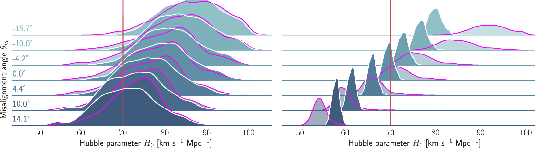
Figure 3. Progression of joint GW+GJ(c)+z Hubble posteriors for  , with θm varying systematically from −16° to 14°. We show the posteriors for
  (white contours) and
  (magenta contours). The posteriors on the left and right represent the results from the inference with the GJ and GJc scenario, respectively.
Download figure:
Standard image High-resolution imageTo assess the presence of model bias, we compare the H0 posterior distributions from fits run on the same data set with different assumed jet models. Table B2 contains the difference in median H0 values from GJ and PLJ runs normalized by the GJ H0 (ΔH0) and by the width σ of the GJ H0 posterior (δ H0). In the no-centroid runs, GJ and PLJ models show a maximum bias of 2% in median H0. This occurs in the θvi = 20° run and corresponds to a 0.49σ bias. All other runs show less than 0.08σ bias. Including astrometric centroid data increases the constraining power of the EM afterglow, increasing the precision of H0 inference, which also increases its vulnerability to bias from model mis-specification. Between the GW+GJc+z and GW+PLJ+z runs, we again find a maximum discrepancy in median H0 of 2%, this time in the θvi = 40° run.
3.2. Angular Mismatch Bias
We now turn our attention to systems that have a nonvanishing line-of-sight misalignment angle and compute joint GW+EM posteriors for the Hubble parameter neglecting this fact; i.e., we will still use θm = 0 in Equation (3). The mock data in the GW sector were set up with this in mind, and we computed several slightly shifted GW posteriors, scattered around the events that were used in Section 3.1. Consequently,  will be fixed, and events with deviating
  are combined in the joint posterior, resulting in a systematic variation of
  . As discussed in Section 1, increasing
  implies that the GW posterior is shifted toward subsequently higher-inclination regions, and the overlap with the EM posterior will occur at larger values of dL
; thus, we expect the H0 posterior to shift toward smaller H0 for greater misalignment
implies that the GW posterior is shifted toward subsequently higher-inclination regions, and the overlap with the EM posterior will occur at larger values of dL
; thus, we expect the H0 posterior to shift toward smaller H0 for greater misalignment  . This behavior is demonstrated in Figure 3 for the posteriors from the GW+GJ(c)+z scenarios at
  and 40°. Two important observations can be made. Clearly, the high-precision posteriors from the GJc analysis (
 ) are more sensitive to the misalignment, and already a small shift of ±4° causes a 2σ–4σ bias in the resulting H0 (see Table B4). Furthermore, we know from Section 3.1 that the posterior for the GJ analysis is biased toward larger H0, which is evident in Figure 3, and we note that a large and positive
  will result in a more accurate Hubble posterior, since the two effects cancel. On the other hand, a small negative
  can amplify the model bias, leading to an even more inaccurate inference. We also confirm this behavior through the change of the 95% credible regions for the cases
  and 40° (see Figure 4), which seem to suggest the general trend that for an inference that is using light-curve and centroid data,
  will lead to a
  bias, which is then quickly increasing for larger magnitudes.
11
For a viewing angle of 20°, we can also state that the inference using only photometry data is less sensitive since
bias, which is then quickly increasing for larger magnitudes.
11
For a viewing angle of 20°, we can also state that the inference using only photometry data is less sensitive since  will not bias the result beyond
  ; however, we cannot make a similar result for the higher-inclination systems shown in Figures 3 and 4, since they have an intrinsic bias that can combine with the misalignment to cause more drastic shifts.
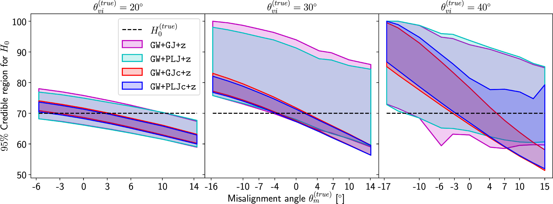
Figure 4. 95% highest posterior density credible regions (2σ) for the Hubble posteriors of all four GW+EM inference scenarios (different scenarios are indicated by red/magenta colored regions for the GJ(c) model and blue/cyan for the PLJ(c) model), with  and
and  and θm varying systematically. The truth is indicated with a dashed line. (Data tabulated in Tables B3 and B4.)
Download figure:
Standard image High-resolution image3.3. Mitigation of Angular Mismatch Bias
Now that we have established that even a small line-of-sight angular mismatch of  can lead to a severely biased Hubble posterior, we want to address a possible method of mitigating this bias. Since we have a well-defined mismatch parameter θm, we can consider this as a nuisance parameter in the joint inference and co-infer it with the Hubble parameter. Marginalization of the posterior in the H0–θm plane should then lead to an unbiased posterior for the Hubble parameter, and we can also obtain a posterior for the mismatch. The key modification is that we treat θm as a variable with an associated prior added to Equation (3). The effect of the misalignment angle is to shift the dL
–θvi posterior/likelihood from the EM inference in the θvi direction without changing its shape. Consequently, in the joint posterior, we will compute a shifted overlap in θJN space in Equation (6). Note that contrary to the behavior of
can lead to a severely biased Hubble posterior, we want to address a possible method of mitigating this bias. Since we have a well-defined mismatch parameter θm, we can consider this as a nuisance parameter in the joint inference and co-infer it with the Hubble parameter. Marginalization of the posterior in the H0–θm plane should then lead to an unbiased posterior for the Hubble parameter, and we can also obtain a posterior for the mismatch. The key modification is that we treat θm as a variable with an associated prior added to Equation (3). The effect of the misalignment angle is to shift the dL
–θvi posterior/likelihood from the EM inference in the θvi direction without changing its shape. Consequently, in the joint posterior, we will compute a shifted overlap in θJN space in Equation (6). Note that contrary to the behavior of  in Section 3.2, θm shifts the EM likelihood with respect to the GW+z likelihood; for θm > 0, it is shifted to larger θvi, leading to a posterior overlap with the GW posterior that occurs at larger inclination than for θm = 0 and therefore at smaller dL
, which will increase the inferred H0. Thus, we expect a direct positive correlation between θm and H0 (see also Figure 2 for a qualitative comparison).
in Section 3.2, θm shifts the EM likelihood with respect to the GW+z likelihood; for θm > 0, it is shifted to larger θvi, leading to a posterior overlap with the GW posterior that occurs at larger inclination than for θm = 0 and therefore at smaller dL
, which will increase the inferred H0. Thus, we expect a direct positive correlation between θm and H0 (see also Figure 2 for a qualitative comparison).
We apply the modified inference to the same cases at  , as shown in Figures 3 and 4, using the prior
 ![$\pi \left({\theta }_{{\rm{m}}}| {\lambda }_{{H}_{0}}\right)={ \mathcal U }\left[-60^\circ ,60^\circ \right]$](https://content.cld.iop.org/journals/2041-8205/977/2/L45/revision1/apjlad8dd1ieqn63.gif) rad for the misalignment angle and considering only the GJ model with or without the centroid. The resulting 2D posteriors in the θm–H0 plane for the cases of
rad for the misalignment angle and considering only the GJ model with or without the centroid. The resulting 2D posteriors in the θm–H0 plane for the cases of  , ±4°, −10°, ±16° are shown in Figure 5. Considering the case of
  first, we observe the expected positive correlation/degeneracy, and both the GW+GJ+z and GW+GJc+z inferences are consistent with the truth to within 1σ, respectively.
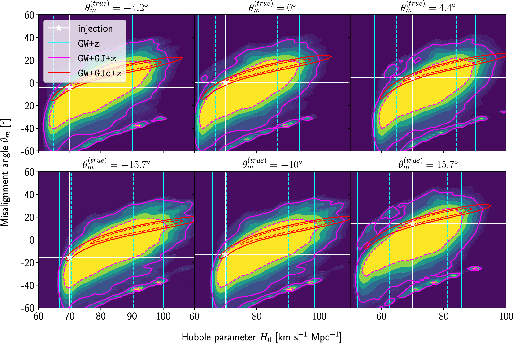
Figure 5. 2D posteriors for the (θm, H0) inference of the  event, with
  , −10°, −4
2, 0°, 4
4, 15
7} from left to right. The heat map represents the GW+GJ+z posterior, while the magenta and red contours indicate the 1σ (dashed) and 2σ (solid) highest posterior density regions for the GW+GJ+z and GW+GJc+z posteriors, respectively. The truths are marked with white stars. We also indicate the 1σ (dashed) and 2σ (solid) regions of the GW+z posteriors with cyan lines.
Download figure:
Standard image High-resolution imageFor the scenarios with intrinsic misalignment, it seems that negative misalignment affects the accuracy worse than positive misalignment, while all posteriors from the GJ data sets lead to a  accuracy, and the large negative misalignments
  are at the edge. This behavior is more pronounced in the inference with the GJc data sets, where all scenarios with
  are only accurate to within 2σ, while positive misalignment still maintains a
  accuracy (see Figures B1 and B2 for statistics of the marginal H0 posteriors). This is related to our choice of using the same noise seed for all GW mock data realizations,
12
which for the considered data shifts the dL
–θvi posterior toward larger inclination angles than the injected value
13
; see the discussion in Section 3.1. Consequently, the combined GW+EM posteriors tend to have higher posterior overlap for positive misalignment angles, thus leading to more posterior support toward θm > 0. However, all posteriors have support over a large region in the θm–H0 plane, and once we compute the marginal posteriors for the Hubble parameter, we shall obtain unconstraining posteriors due to the degeneracy of θm and H0. The statistics for the marginal H0 posteriors in Figure 5 demonstrate that the precision, even for the most constraining EM data sets (GJc), is reduced to within a factor of 1.1–1.2 of the level of the GW+z posteriors (see second column in Figure B2).
accuracy (see Figures B1 and B2 for statistics of the marginal H0 posteriors). This is related to our choice of using the same noise seed for all GW mock data realizations,
12
which for the considered data shifts the dL
–θvi posterior toward larger inclination angles than the injected value
13
; see the discussion in Section 3.1. Consequently, the combined GW+EM posteriors tend to have higher posterior overlap for positive misalignment angles, thus leading to more posterior support toward θm > 0. However, all posteriors have support over a large region in the θm–H0 plane, and once we compute the marginal posteriors for the Hubble parameter, we shall obtain unconstraining posteriors due to the degeneracy of θm and H0. The statistics for the marginal H0 posteriors in Figure 5 demonstrate that the precision, even for the most constraining EM data sets (GJc), is reduced to within a factor of 1.1–1.2 of the level of the GW+z posteriors (see second column in Figure B2).
Considering the most precise posteriors that are obtained from analyzing light-curve and centroid data, we obtain  constraints for H0 from marginalizing θm in the 2D posteriors in Figure 5, which is comparable to the constraints obtained by only fitting the light curve in the cases with zero misalignment in Section 3.1. We also compute 2D posteriors in the θm–H0 plane for the series of events without misalignment that was considered in Section 3.1, where we would expect to obtain an accurate inference of H0 with the maximum posterior region centered around θm = 0. This is indeed what we find; θm is constrained to 0 with
  precision, and we obtain Hubble posteriors that are accurate to within 1.5σ for all viewing angles
  . The posterior statistics are summarized in Table B5 and the second column of Figure B3 in Appendix B. However, also for these scenarios, the gain in precision from including EM data is reduced due to marginalization of the misalignment angle; see the second column of Figure B3 for more details.
Trusting the theoretical models, we might expect that the physical misalignment will be of  at most; consequently, a narrower choice for the θm prior could be motivated, e.g.,
 ![$\pi \left({\theta }_{{\rm{m}}}| {\lambda }_{{H}_{0}}\right)={ \mathcal U }\left[-10^\circ ,10^\circ \right]$](https://content.cld.iop.org/journals/2041-8205/977/2/L45/revision1/apjlad8dd1ieqn76.gif) , and this could also reduce the spread in the posterior while still being able to confidently infer the misalignment in the cases with
, and this could also reduce the spread in the posterior while still being able to confidently infer the misalignment in the cases with  . We have applied the same bias-mitigating procedure as discussed above to data sets with
  , −4
, −42, 0°, 4
4, 6
2}, but we applied the narrower prior range for θm, and the statistics for the marginal H0 posterior indeed show that for the posteriors from the GJc data sets, the accuracy behaves similar to the case with a wider θm prior, but the precision is again improved to a factor of 2 compared to the GW+z posteriors (Figure B4, as well as the third column in Figure B2). This demonstrates the need for narrow theoretical bounds for the misalignment angle in the joint inference of H0, for the amount of precision that can be achieved in the single-event-level inference of H0 in this scenario is directly linked to the prior width in H0.
4. Conclusion and Future Outlook
In this work, we analyze scenarios for the joint inference of the Hubble parameter from GW and EM data at the single-event level that attempt to mimic a realistic multimessenger campaign in the near future, in terms of available data and models, under ideal conditions. We point out a potential source of bias in the inference of the value of H0 from multimessenger observation due to incorrect model fitting with EM observations and/or intrinsic misalignment between the inclination angle and the jet angle. For the case of incorrect modeling, we find that over the range θvi = 3°–40°, the model bias is a subdominant effect, as both assumptions on the jet structure lead to consistent results to within  , extending the findings for a GW170817-like event in G. Gianfagna et al. (2024). GJc/PLJc are precise and accurate for θvi = 3°–40°, while GJ/PLJ are precise and accurate for θvi = 3°–20° (although already worse by a factor of 3 than the analysis with centroid data) but less precise (
 ) and inaccurate at θvi = 30°–40°, with an
  overestimation, which can be prohibitive for cosmological inference.
On the other hand, the physical misalignment between the orbital angular momentum axis of the inspiraling binary and the jet axis was identified as a significant source of bias in the joint inference of GW and EM data, particularly when centroid information is included. Data with line-of-sight misalignment  that are analyzed under the assumption of alignment—which is frequently employed (see B. P. Abbott et al. 2017c; H.-Y. Chen et al. 2019; A. Farah et al. 2020), as the misalignment is not constrained by current theoretical models—can lead to
  biases in H0, corresponding to 3%–7% deviations for
  and 5%–12% for
  . This shows that presently used models for the EM counterpart lead to posteriors that are even more sensitive than what was found by H.-Y. Chen (2020) based on Gaussian estimates. Since we are using superideal events, this is a lower limit, and it is already close to the required accuracy for resolving the Hubble tension at about ≳3σ (e.g., K. Hotokezaka et al. 2019). Ensuring an accurate H0 inference from bright sirens would therefore require a method to mitigate such systematic biases.
Note that random values of misalignment for a large number of events would also cause random systematic errors in H0, and if multiple events were combined, their effects might average out to provide an unbiased H0. However, the prospects for observing many BNS or BHNS mergers that can be analyzed with the bright sirens method are limited, and the expectation is that analyses in the near future will have access to a few events at best; see, e.g., G. Gianfagna et al. (2024). In this case, even a few observations with precise but inaccurate H0 posteriors from the inclusion of light-curve and centroid data could dominate over other bright siren measurements of H0 that only have access to the redshift, and the bias of the multievent inference would be driven by the systematic errors in the analysis at the single-event level. Consequently, it is paramount to identify biases at the single-event level and to reduce these if possible.
To mitigate the uncertainty due to the model or misalignment biases, one is required to jointly infer the value of θm and H0 to obtain an unbiased marginal posterior on H0 and also an inference of θm . The multimessenger observations from GW and EM data are capable of providing information on θm , and our analysis shows that they should be inferred together, rather than assuming the value of θm to be 0. The later assumption can cause a biased H0 even for a minor deviation that is easily feasible astrophysically (e.g., N. Stone et al. 2013; H. Nagakura et al. 2014; K. Hayashi et al. 2022; Y. Li et al. 2023).
We conclude that co-inferring and marginalizing over the misalignment angle can indeed reduce the bias in the inferred H0 to within 2σ but at the cost of the precision that is available at the single-event level. If the misalignment angle is given a wide prior range, this can reduce the precision of the GW+EM inference to the level of the GW-only inference, thus removing the benefit of the combined analysis for the considered scenarios. However, this might change at larger redshifts, depending on the quality of the EM data compared to the GW data. Reducing the prior range for θm can restore the gain in precision for the combined GW+EM inference up to a factor of 2 with respect to the GW+z posteriors; thus, improvements on the theoretical bracket for this parameter will be paramount for ensuring a highly constraining and unbiased inference.
In the future, it will be important to incorporate this analysis in the bright siren studies for which EM measurements of the viewing angle from light-curve and/or centroid data are available. Along with the inference of H0, this technique makes it possible to also infer the value of the mismatch angle θm . This can be useful in understanding the astrophysical properties of BNS/BHNS mergers better, shedding light on to what extent merger-driven jets are aligned with the orbital angular momentum. With a population of BNS/BHNS events, a population-level inference of θm can lead to new insights about the complexity of the postmerger phase.
Acknowledgments
The authors thank Samsuzzaman Afroz for useful comments on the draft. This research was supported in part by the Perimeter Institute for Theoretical Physics. Research at the Perimeter Institute is supported in part by the Government of Canada through the Department of Innovation, Science and Economic Development and by the Province of Ontario through the Ministry of Colleges and Universities. M.M. acknowledges the support of NSERC, funding reference No. RGPIN-2019-04684. The work of S.M. is part of the 〈data∣theory〉 Universe-Lab, supported by TIFR and the Department of Atomic Energy, Government of India. The authors express gratitude to the computer cluster of 〈data∣theory〉 Universe-Lab. The authors would like to thank the LIGO/Virgo/KAGRA scientific collaboration for providing the data. LIGO is funded by the U.S. National Science Foundation. Virgo is funded by the French Centre National de Recherche Scientifique (CNRS), the Italian Istituto Nazionale della Fisica Nucleare (INFN), and the Dutch Nikhef, with contributions by Polish and Hungarian institutes. This material is based upon work supported by NSF’s LIGO Laboratory, which is a major facility fully funded by the National Science Foundation.
Appendix A: EM Mock Data Generation
GRB afterglows are produced by synchrotron emission from a nonthermal electron population, accelerated at the forward shock driven by the GRB jet. The jet launching mechanism imbues the jet with a distribution of energy E(θ), typically taken to be axisymmetric. The jet sweeps up the ambient medium of density n0, forms a shock, decelerates, and spreads laterally. As first-principles simulations of BNS mergers have not converged on a jet structure, we instead use simple phenomenological models: a GJ  and a PLJ
  . Both have central energy E0 and core width θc
and are truncated at an outer angle θw
; the PLJ also includes an index b.
. Both have central energy E0 and core width θc
and are truncated at an outer angle θw
; the PLJ also includes an index b.
Following standard afterglow theory (e.g., J. Granot & R. Sari 2002), the nonthermal electrons acquire a power-law energy distribution of index −p, made up of a fraction ξN
of the available electrons. The nonthermal electrons and the magnetic field are each assigned fractions e
and
B
, respectively, of the available shock energy. The GRB is placed at redshift z and luminosity distance dL
and oriented θvi relative to Earth. For pure photometric data, this is enough to compute a flux; for astrometric centroid data, we also need initial sky coordinates RA0 and Dec0 and a PA on the sky.
We use the fiducial GJ model of G. Ryan et al. (2024) for the generation of light curves. This model is consistent with the GW170817 afterglow observations and has the parameters E0 = 4.8 × 1053 erg, θc
= 32, θw
= 22
4, n0 = 2.4 × 10⁻³ cm−3, p = 2.13,
e
= 1.9 × 10⁻³,
B
= 5.8 × 10⁻⁴, and ξN
= 0.95. Emission from this jet model is computed using afterglowpy v0.8.0 with jet spreading enabled; see G. Ryan et al. (2020, 2024) for implementation details.
We generate mock data from the fluxes of the injected GJ by simulating an idealized observation campaign using radio, optical, and X-ray photometric observations as well as radio observations of the centroid position. We designed the data-generation algorithm to roughly model an optimistic observation scenario for a GW EM counterpart.
The procedure goes as follows: for each photometric band, we space observations geometrically between 1 and 104 days postmerger. Starting at t = 1 day, we compute the model flux, add noise, and determine whether our mock observatory would detect the emission. If the source is undetected, an upper limit is recorded, and the next observation is attempted a factor of 101/2 ≈ 3.1 later in time, giving these monitoring observations a cadence of two per decade in time. If at any time the source is detected, a flux observation with the relevant uncertainty is recorded, and the next observation is scheduled a factor of 101/4 ≈ 1.8 later in time, giving an observing cadence of four per decade in time. Once the afterglow is detected in a band, “observations” continue in that band at the four-per-decade cadence until two successive upper limits are found, at which point observations in that band cease. Radio very long baseline interferometry (VLBI) observations are carried out between 10 and 104 days postmerger at the two-observations-per-decade cadence. This approach generates sufficiently dense observations to measure the initial rising slope of the light curve (if the emission is sufficiently bright) and covers a duration of time over which the jet break is expected to appear. These two features contain the most geometric information in the light curve and, if detectable, are essential for extracting the inclination from GRB afterglow observations.
Our mock radio, optical, and X-ray observatories emulate optimistic observations from the Very Large Array (VLA), the Hubble Space Telescope (HST), and Chandra, respectively, with uncertainties and noise levels similar to what was obtained with GW170817 (e.g., W. Fong et al. 2019; E. Troja et al. 2021). We characterize the radio and optical observatories with a flux limit  (representing the noise level of the instrument) and a fractional source uncertainty δ (representing calibration and background-subtraction uncertainties). We assign a total uncertainty to each observation by simply adding these in quadrature:
  , where Fsrc is the model afterglow flux. The synthetic observed flux Fobs is Fsrc plus a random noise contribution drawn from a normal distribution of mean 0 and width σ. If
  , the observation is declared a nondetection, and we emit an upper limit of
  . Otherwise, the observation is a detection, and we emit Fobs with the uncertainty σ. In parameter estimation, these observations are assigned a Gaussian likelihood. Our radio photometry is generated at ν = 3 GHz with δ = 0.05 and
  μJy, representing a long integration by a VLA-like instrument. Our optical photometry is generated at ν = 5.1 × 10¹⁴ Hz with δ = 0.05 and
  nJy, representing a long integration by an HST-like instrument in the F606W filter.
Since many of these sources are faint, we generate mock X-ray data with Poisson statistics unless we exceed 100 observed counts. For each observation, we compute Fsrc at 5 keV and convert this to an expected number of counts S by multiplying by a flux-to-counts conversion factor of 1.4 × 10⁸ mJy−1, a typical value for a 100 ks Chandra observation of GW170817 (E. Troja et al. 2021). We then draw a random background count B from a normal distribution of mean 1.0 and width 0.5, truncated to B > 0 (again, typical for GW170817). The observed photon count N is then drawn from a Poisson distribution with mean B + S. If N > 100, we replace this Poisson observation with a normally distributed flux observation of width 0.1 × Fsrc. In parameter estimation, X-ray observations are assigned a Poisson likelihood following the approach of G. Ryan et al. (2024) unless N > 100, in which case a Gaussian likelihood is used.
Each synthetic VLBI observation produces both a flux and sky coordinates (R.A. and decl.) with relevant uncertainties. The flux observation proceeds identically to the radio photometric routine. The uncertainty σc
in each direction of the centroid is computed as  , where the signal-to-noise ratio (SNR) is Fobs/σ. We compute the true R.A. and decl. from afterglowpy and then add Gaussian noise of width σc
to produce the observed values. As in the mock photometry, if
, where the signal-to-noise ratio (SNR) is Fobs/σ. We compute the true R.A. and decl. from afterglowpy and then add Gaussian noise of width σc
to produce the observed values. As in the mock photometry, if  , the observation is declared a nondetection, a 3σ flux upper limit is emitted, and the R.A. and decl. uncertainties are set to large numbers to make the data points unconstraining. We take the flux uncertainty parameters as above and assign an optimistic σbeam = 1 mas. In parameter estimation, the flux, R.A., and decl. are given a 3D multivariate normal likelihood with independent uncertainties (a diagonal covariance matrix).
For the fitting of the mock data, we employ the following prior ranges in  , θc
, θw
, b,
, θc
, θw
, b,  , p,
, p,  ,
,  ,
,  , RA0, Dec0, PA}:
 ![${ \mathcal U }\left[45,56\right]$](https://content.cld.iop.org/journals/2041-8205/977/2/L45/revision1/apjlad8dd1ieqn101.gif) ,
, ![${ \mathcal U }\left[0.01,\pi /2\right]$](https://content.cld.iop.org/journals/2041-8205/977/2/L45/revision1/apjlad8dd1ieqn102.gif) rad,
rad, ![${ \mathcal U }\left[0.01,\pi /2\right]$](https://content.cld.iop.org/journals/2041-8205/977/2/L45/revision1/apjlad8dd1ieqn103.gif) rad,
rad, ![${ \mathcal U }\left[0,10\right]$](https://content.cld.iop.org/journals/2041-8205/977/2/L45/revision1/apjlad8dd1ieqn104.gif) ,
, ![${ \mathcal U }\left[-6,10\right]$](https://content.cld.iop.org/journals/2041-8205/977/2/L45/revision1/apjlad8dd1ieqn105.gif) ,
, ![${ \mathcal U }\left[2,5\right]$](https://content.cld.iop.org/journals/2041-8205/977/2/L45/revision1/apjlad8dd1ieqn106.gif) ,
, ![${ \mathcal U }\left[-6,0\right]$](https://content.cld.iop.org/journals/2041-8205/977/2/L45/revision1/apjlad8dd1ieqn107.gif) ,
, ![${ \mathcal U }\left[-6,0\right]$](https://content.cld.iop.org/journals/2041-8205/977/2/L45/revision1/apjlad8dd1ieqn108.gif) ,
, ![${ \mathcal U }\left[-6,0\right]$](https://content.cld.iop.org/journals/2041-8205/977/2/L45/revision1/apjlad8dd1ieqn109.gif) ,
, ![${ \mathcal U }\left[-10,10\right]$](https://content.cld.iop.org/journals/2041-8205/977/2/L45/revision1/apjlad8dd1ieqn110.gif) mas,
mas, ![${ \mathcal U }\left[-10,10\right]$](https://content.cld.iop.org/journals/2041-8205/977/2/L45/revision1/apjlad8dd1ieqn111.gif) mas,
mas, ![${ \mathcal U }\left[0^\circ ,360^\circ \right]$](https://content.cld.iop.org/journals/2041-8205/977/2/L45/revision1/apjlad8dd1ieqn112.gif) . Furthermore, the EM inference uses the same prior for the viewing angle as is used for the inclination in the λGW model, i.e.,
. Furthermore, the EM inference uses the same prior for the viewing angle as is used for the inclination in the λGW model, i.e.,  , but with range θvi ∈ [0, π/2], and for the distance prior, we use a Gaussian prior in H0 that is centered on a fixed value of
  km s−1 Mpc−1, i.e.,
  (in km s−1 Mpc−1), where
  denotes a Gaussian distribution with mean μ and variance σ. This prior then induces a prior on the luminosity distance, which can be obtained in closed form if we assume that we are at small redshifts where the luminosity distance is not sensitive to the specific cosmological model and
  , in which case
  , for constant redshift. This is chosen to limit the range in dL
beyond the
, for constant redshift. This is chosen to limit the range in dL
beyond the ![${ \mathcal U }\left[1,100\right]$](https://content.cld.iop.org/journals/2041-8205/977/2/L45/revision1/apjlad8dd1ieqn119.gif) Mpc prior that was specified above, since a large range in dL
reduces the efficiency of the inference. We made sure that the precision of the dL
posteriors from the EM data is always worse than the GW constraints, such that the joint inference is not affected by this choice.
Mpc prior that was specified above, since a large range in dL
reduces the efficiency of the inference. We made sure that the precision of the dL
posteriors from the EM data is always worse than the GW constraints, such that the joint inference is not affected by this choice.
Figure A1 shows the generated mock light-curve observations for this work.

Figure A1. We show the light-curve data for the used EM counterparts, generated with a GJ. The different frequency bands are color coded (red: radio; blue: optical; violet: X-ray), and measurements are plotted with an error bar, while upper limits are denoted with an upside-down triangle.
Download figure:
Standard image High-resolution imageAppendix B: Supplemental Tables
In this section, we summarize the results from the different inference campaigns. For every campaign, we quote the median (![$\mathrm{med}\left[{H}_{0}\right]$](https://content.cld.iop.org/journals/2041-8205/977/2/L45/revision1/apjlad8dd1ieqn120.gif) ) and the 2.5th–97.5th percentiles of the H0 posteriors for the different inference scenarios. Furthermore, we provide statistics that help to estimate the accuracy and precision of the respective posteriors, we use
) and the 2.5th–97.5th percentiles of the H0 posteriors for the different inference scenarios. Furthermore, we provide statistics that help to estimate the accuracy and precision of the respective posteriors, we use ![${{\rm{\Gamma }}}_{{H}_{0}}={\sigma }_{{H}_{0}}/\mathrm{med}\left[{H}_{0}\right]$](https://content.cld.iop.org/journals/2041-8205/977/2/L45/revision1/apjlad8dd1ieqn121.gif) to gauge the precision (statistical error) of the measurement, and, since we know the truth in our runs, we define
to gauge the precision (statistical error) of the measurement, and, since we know the truth in our runs, we define ![${\beta }_{{H}_{0}}=(\mathrm{med}\left[{H}_{0}\right]-{H}_{0}^{(\mathrm{true})})/{\sigma }_{{H}_{0}}$](https://content.cld.iop.org/journals/2041-8205/977/2/L45/revision1/apjlad8dd1ieqn122.gif) to estimate the accuracy.
to estimate the accuracy.
To better understand the differences/consistency between different inference models for the EM data, we also define the quantities ![${\rm{\Delta }}{H}_{0}=(\mathrm{med}{\left[{H}_{0}\right]}_{\mathrm{GJ}({\rm{c}})}-\mathrm{med}{\left[{H}_{0}\right]}_{\mathrm{PLJ}({\rm{c}})})/\mathrm{med}{\left[{H}_{0}\right]}_{\mathrm{GJ}({\rm{c}})}$](https://content.cld.iop.org/journals/2041-8205/977/2/L45/revision1/apjlad8dd1ieqn123.gif) for the relative deviation from the GJ(c) model and
for the relative deviation from the GJ(c) model and ![$\delta {H}_{0}\,=\mathrm{med}{\left[{H}_{0}\right]}_{\mathrm{GJ}({\rm{c}})}{\rm{\Delta }}{H}_{0}/{\sigma }_{{H}_{0}}^{\mathrm{GJ}}$](https://content.cld.iop.org/journals/2041-8205/977/2/L45/revision1/apjlad8dd1ieqn124.gif) for the deviation from GJ(c) in terms of
for the deviation from GJ(c) in terms of  , in analogy to our accuracy statistic
  . We check consistency only among light-curve-only and light curve + centroid motion inferences, respectively, and we always use the GJ(c) jet models as a reference, since these should also be consistent with the injection.
We work with unrealistically close and therefore loud sources, which will suppress the statistical error (estimated in terms of  ) to be able to identify systematic errors which might be hidden for sources with higher statistical errors (there the bias would only show up on the multievent level, once the statistical error reaches the bias scale). We choose the sources so close that the statistical error is below the bias scale that could still be problematic for the desired precision, any bias that we do not resolve at this point would also not become relevant for the immediate Hubble inference. This implies that
  and ΔH0 do not provide representative properties of the posteriors that would generalize to more realistic sources. Only
  and δ
H0, which are normalized by the statistical error, would provide an idea of how the distributions might change for larger statistical errors.
and δ
H0, which are normalized by the statistical error, would provide an idea of how the distributions might change for larger statistical errors.
In Tables B1 and B2, we show the statistics for the inference runs that do not use an intrinsic misalignment parameter and where the only inaccuracy can arise from a biased EM inference.
Table B1. Inferred Hubble Parameter for Different Inference Scenarios with Zero Misalignment Angle in the Datasets

| H0 (Median, 2.5th–97.5th percentiles) | ||||
|---|---|---|---|---|---|
| GW+z | GW+GJ+z | GW+PLJ+z | GW+GJc+z | GW+PLJc+z | |
| 3° |

|

|

|

|

|
| 10° |

|

|

|

|

|
| 20° |

|

|

|

|

|
| 30° |

|

|

|

|

|
| 40° |

|

|

|

|

|
| 50° |

|

|

|

|

|
| 60° |

|

|

|

|

|
| 70° |

|

|

|

|

|
| 80° |

|

|

|

|

|
Note. This table lists the posterior results for the Hubble parameter from the  inference campaign for the different inference scenarios and all viewing angles using the median of the posterior distribution and the 2.5th–97.5th percentiles.
Download table as: ASCIITypeset image
Table B2. Precision and Accuracy of the Inferred Hubble Parameter for Different Inference Scenarios with Zero Misalignment Angle in the Datasets

| H0 (Median, 2.5th–97.5th percentiles) | Posterior Consistency | ||||||||||||
|---|---|---|---|---|---|---|---|---|---|---|---|---|---|---|
| GW+z | GW+GJ+z | GW+PLJ+z | GW+GJc+z | GW+PLJc+z | GJ/PLJ | GJc/PLJc | ||||||||

|

|

|

|

|

|

|

|

|

| ΔH0 | δ H0 | ΔH0 | δ H0 | |
| 3° | 0.1 | 1.8 | 0.01 | −0.51 | 0.01 | −0.43 | 0.01 | −0.53 | 0.01 | −0.4 | −0.0 | −0.07 | −0.0 | −0.12 |
| 10° | 0.1 | 1.69 | 0.01 | −0.53 | 0.02 | −0.36 | 0.01 | 0.03 | 0.01 | 0.03 | −0.0 | −0.07 | −0.0 | −0.01 |
| 20° | 0.11 | 1.29 | 0.04 | 0.24 | 0.03 | −0.26 | 0.01 | 0.13 | 0.01 | −0.33 | 0.02 | 0.49 | 0.01 | 0.46 |
| 30° | 0.12 | 0.84 | 0.09 | 1.39 | 0.08 | 1.45 | 0.02 | −0.32 | 0.01 | −0.65 | 0.01 | 0.08 | 0.0 | 0.3 |
| 40° | 0.12 | 0.33 | 0.1 | 1.17 | 0.1 | 1.21 | 0.04 | 0.48 | 0.05 | 0.77 | −0.0 | −0.03 | −0.02 | −0.45 |
| 50° | 0.12 | 0.15 | 0.1 | 0.57 | 0.1 | 0.55 | 0.1 | 0.5 | 0.11 | 0.51 | 0.0 | 0.02 | −0.0 | −0.03 |
| 60° | 0.09 | 0.2 | 0.08 | 0.49 | 0.08 | 0.49 | 0.08 | 0.43 | 0.08 | 0.45 | 0.0 | 0.01 | −0.0 | −0.03 |
| 70° | 0.05 | 0.33 | 0.04 | 0.62 | 0.04 | 0.63 | 0.04 | 0.6 | 0.05 | 0.61 | −0.0 | −0.01 | −0.0 | −0.02 |
| 80° | 0.02 | 0.18 | 0.02 | 0.7 | 0.02 | 0.72 | 0.02 | 0.72 | 0.02 | 0.74 | −0.0 | −0.03 | −0.0 | −0.02 |
Note. This table lists statistics for the Hubble posterior from the  inference campaign for the different inference scenarios and all viewing angles with two decimal places (0.0 means a number <0.01). We quote
 ![${{\rm{\Gamma }}}_{{H}_{0}}={\sigma }_{{H}_{0}}/\mathrm{med}\left[{H}_{0}\right]$](https://content.cld.iop.org/journals/2041-8205/977/2/L45/revision1/apjlad8dd1ieqn189.gif) (for precision),
(for precision), ![${\beta }_{{H}_{0}}=(\mathrm{med}\left[{H}_{0}\right]-{H}_{0}^{(\mathrm{true})})/{\sigma }_{{H}_{0}}$](https://content.cld.iop.org/journals/2041-8205/977/2/L45/revision1/apjlad8dd1ieqn190.gif) (for accuracy),
(for accuracy), ![${\rm{\Delta }}{H}_{0}=(\mathrm{med}{\left[{H}_{0}\right]}_{\mathrm{GJ}({\rm{c}})}-\mathrm{med}{\left[{H}_{0}\right]}_{\mathrm{PLJ}({\rm{c}})})/\mathrm{med}{\left[{H}_{0}\right]}_{\mathrm{GJ}({\rm{c}})}$](https://content.cld.iop.org/journals/2041-8205/977/2/L45/revision1/apjlad8dd1ieqn191.gif) (for relative deviation the from GJ(c) model), and
(for relative deviation the from GJ(c) model), and ![$\delta {H}_{0}=\mathrm{med}{\left[{H}_{0}\right]}_{\mathrm{GJ}({\rm{c}})}{\rm{\Delta }}{H}_{0}/{\sigma }_{{H}_{0}}^{\mathrm{GJ}}$](https://content.cld.iop.org/journals/2041-8205/977/2/L45/revision1/apjlad8dd1ieqn192.gif) (for deviation from GJ(c) in terms of
(for deviation from GJ(c) in terms of  ).
).
Download table as: ASCIITypeset image
In Tables B3 and B4, we show the statistics for the H0 posteriors in Figure 4, which varies the intrinsic misalignment systematically around the aligned case for low-to-intermediate θvi.
Table B3. Inferred Hubble Parameter for Different Inference Scenarios with Nonzero Misalignment Angle in the Datasets

|
| H0 (Median, 2.5th–97.5th percentiles) | |||
|---|---|---|---|---|---|
| GW+GJ+z | GW+PLJ+z | GW+GJc+z | GW+PLJc+z | ||
| 20° | −6° |

|

|

|

|
| −3° |

|

|

|

| |
| 0° |

|

|

|

| |
| 3° |

|

|

|

| |
| 6° |

|

|

|

| |
| 10° |

|

|

|

| |
| 14° |

|

|

|

| |
| 30° | −16° |

|

|

|

|
| −13° |

|

|

|

| |
| −10° |

|

|

|

| |
| −7° |

|

|

|

| |
| −4° |

|

|

|

| |
| 0° |

|

|

|

| |
| 4° |

|

|

|

| |
| 7° |

|

|

|

| |
| 10° |

|

|

|

| |
| 14° |

|

|

|

| |
| 40° | −17° |

|

|

|

|
| −14° |

|

|

|

| |
| −10° |

|

|

|

| |
| −6° |

|

|

|

| |
| −3° |

|

|

|

| |
| 0° |

|

|

|

| |
| 4° |

|

|

|

| |
| 7° |

|

|

|

| |
| 10° |

|

|

|

| |
| 13° |

|

|

|

| |
| 15° |

|

|

|

| |
Note. This table lists the median and 2.5th–97.5th percentiles of the posterior results for the Hubble parameter from the  data sets at varying
  , shown in Figure 4.
Download table as: ASCIITypeset image
Table B4. Precision and Accuracy of the Inferred Hubble Parameter for Different Inference Scenarios with Nonzero Misalignment Angle in the Datasets

|

| H0 Posterior Statistics | Posterior Consistency | ||||||||||
|---|---|---|---|---|---|---|---|---|---|---|---|---|---|
| GW+GJ+z | GW+PLJ+z | GW+GJc+z | GW+PLJc+z | GJ/PLJ | GJc/PLJc | ||||||||

|

|

|

|

|

|

|

| ΔH0 | δ H0 | ΔH0 | δ H0 | ||
| 20° | −6° | 0.04 | 1.05 | 0.03 | 0.62 | 0.01 | 3.02 | 0.01 | 2.52 | 0.02 | 0.49 | 0.01 | 0.49 |
| −3° | 0.04 | 0.69 | 0.03 | 0.22 | 0.01 | 1.73 | 0.01 | 1.25 | 0.02 | 0.49 | 0.01 | 0.47 | |
| 0° | 0.04 | 0.24 | 0.03 | −0.26 | 0.01 | 0.13 | 0.01 | −0.33 | 0.02 | 0.49 | 0.01 | 0.46 | |
| 3° | 0.04 | −0.43 | 0.03 | −0.94 | 0.01 | −2.11 | 0.01 | −2.53 | 0.02 | 0.48 | 0.0 | 0.43 | |
| 6° | 0.03 | −0.96 | 0.04 | −1.39 | 0.01 | −3.93 | 0.01 | −4.33 | 0.01 | 0.42 | 0.0 | 0.42 | |
| 10° | 0.03 | −2.03 | 0.04 | −2.26 | 0.01 | −6.8 | 0.01 | −7.16 | 0.01 | 0.37 | 0.0 | 0.33 | |
| 14° | 0.03 | −3.29 | 0.04 | −3.4 | 0.01 | −11.18 | 0.01 | −11.53 | 0.01 | 0.38 | 0.0 | 0.34 | |
| 30° | −16° | 0.08 | 2.53 | 0.07 | 2.68 | 0.02 | 6.67 | 0.02 | 6.97 | 0.01 | 0.11 | 0.01 | 0.41 |
| −13° | 0.08 | 2.28 | 0.07 | 2.41 | 0.02 | 5.95 | 0.02 | 6.13 | 0.01 | 0.11 | 0.01 | 0.4 | |
| −10° | 0.08 | 2.1 | 0.07 | 2.21 | 0.02 | 5.06 | 0.02 | 5.1 | 0.01 | 0.12 | 0.01 | 0.39 | |
| −7° | 0.08 | 1.89 | 0.07 | 2.0 | 0.02 | 3.64 | 0.02 | 3.51 | 0.01 | 0.11 | 0.01 | 0.36 | |
| −4° | 0.08 | 1.68 | 0.08 | 1.77 | 0.02 | 2.4 | 0.02 | 2.17 | 0.01 | 0.1 | 0.01 | 0.35 | |
| 0° | 0.09 | 1.39 | 0.08 | 1.45 | 0.02 | −0.32 | 0.01 | −0.65 | 0.01 | 0.08 | 0.0 | 0.3 | |
| 4° | 0.09 | 0.97 | 0.08 | 0.95 | 0.01 | −4.08 | 0.01 | −4.47 | 0.01 | 0.1 | 0.0 | 0.29 | |
| 7° | 0.09 | 0.85 | 0.09 | 0.75 | 0.01 | −6.18 | 0.01 | −6.53 | 0.01 | 0.14 | 0.0 | 0.22 | |
| 10° | 0.09 | 0.52 | 0.09 | 0.42 | 0.01 | −9.31 | 0.01 | −9.7 | 0.01 | 0.13 | 0.0 | 0.16 | |
| 14° | 0.1 | 0.2 | 0.09 | 0.08 | 0.01 | −14.51 | 0.01 | −14.62 | 0.01 | 0.12 | 0.0 | 0.01 | |
| 40° | −17° | 0.09 | 2.23 | 0.09 | 2.33 | 0.04 | 5.67 | 0.04 | 6.26 | −0.01 | −0.08 | −0.01 | −0.26 |
| −14° | 0.09 | 2.05 | 0.09 | 2.16 | 0.05 | 4.82 | 0.04 | 5.4 | −0.01 | −0.08 | −0.01 | −0.3 | |
| −10° | 0.09 | 1.82 | 0.09 | 1.84 | 0.05 | 3.62 | 0.05 | 3.92 | −0.0 | −0.02 | −0.02 | −0.35 | |
| −6° | 0.1 | 1.38 | 0.1 | 1.45 | 0.05 | 2.36 | 0.05 | 2.58 | −0.0 | −0.0 | −0.02 | −0.42 | |
| −3° | 0.1 | 1.36 | 0.1 | 1.41 | 0.05 | 1.67 | 0.05 | 1.86 | −0.0 | −0.01 | −0.02 | −0.45 | |
| 0° | 0.1 | 1.17 | 0.1 | 1.21 | 0.04 | 0.48 | 0.05 | 0.77 | −0.0 | −0.03 | −0.02 | −0.45 | |
| 4° | 0.1 | 1.01 | 0.1 | 1.01 | 0.04 | −1.36 | 0.06 | −0.57 | 0.0 | 0.01 | −0.02 | −0.53 | |
| 7° | 0.1 | 0.86 | 0.1 | 0.87 | 0.04 | −2.95 | 0.07 | −1.39 | −0.0 | −0.02 | −0.02 | −0.52 | |
| 10° | 0.09 | 0.73 | 0.09 | 0.75 | 0.04 | −4.09 | 0.09 | −1.6 | −0.0 | −0.03 | −0.02 | −0.54 | |
| 13° | 0.09 | 0.67 | 0.09 | 0.74 | 0.05 | −4.88 | 0.11 | −1.89 | −0.01 | −0.07 | −0.03 | −0.56 | |
| 15° | 0.09 | 0.57 | 0.08 | 0.7 | 0.06 | −4.59 | 0.12 | −1.96 | −0.01 | −0.11 | −0.04 | −0.69 | |
Note. This table lists statistics for the Hubble posterior from the  data sets at varying
  , shown in Figure 4, for the different inference campaigns and all viewing angles with two decimal places (0.0 means a number <0.01). We quote
 ![${{\rm{\Gamma }}}_{{H}_{0}}={\sigma }_{{H}_{0}}/\mathrm{med}\left[{H}_{0}\right]$](https://content.cld.iop.org/journals/2041-8205/977/2/L45/revision1/apjlad8dd1ieqn322.gif) (for precision),
(for precision), ![${\beta }_{{H}_{0}}=(\mathrm{med}\left[{H}_{0}\right]-{H}_{0}^{(\mathrm{true})})/{\sigma }_{{H}_{0}}$](https://content.cld.iop.org/journals/2041-8205/977/2/L45/revision1/apjlad8dd1ieqn323.gif) (for accuracy),
(for accuracy), ![${\rm{\Delta }}{H}_{0}=(\mathrm{med}{\left[{H}_{0}\right]}_{\mathrm{GJ}({\rm{c}})}-\mathrm{med}{\left[{H}_{0}\right]}_{\mathrm{PLJ}({\rm{c}})})/\mathrm{med}{\left[{H}_{0}\right]}_{\mathrm{GJ}({\rm{c}})}$](https://content.cld.iop.org/journals/2041-8205/977/2/L45/revision1/apjlad8dd1ieqn324.gif) (for relative deviation from the GJ(c) model), and
(for relative deviation from the GJ(c) model), and ![$\delta {H}_{0}=\mathrm{med}{\left[{H}_{0}\right]}_{\mathrm{GJ}({\rm{c}})}{\rm{\Delta }}{H}_{0}/{\sigma }_{{H}_{0}}^{\mathrm{GJ}}$](https://content.cld.iop.org/journals/2041-8205/977/2/L45/revision1/apjlad8dd1ieqn325.gif) (for deviation from GJ(c) in terms of
(for deviation from GJ(c) in terms of  ).
).
Figure B1 and the second column in Figure B2 show the statistics for the marginal H0 posteriors from the bias-mitigating inference of H0 and θm with a subsequent marginalization over θm (we shall hereafter refer to this as  inference). In particular, we consider scenarios where we combine
  with varying values of
  , which are also shown in Figure 5. This complements the previous inferences with
  , where we assumed
  , and obtained the biased posteriors in Figures 3 and 4.
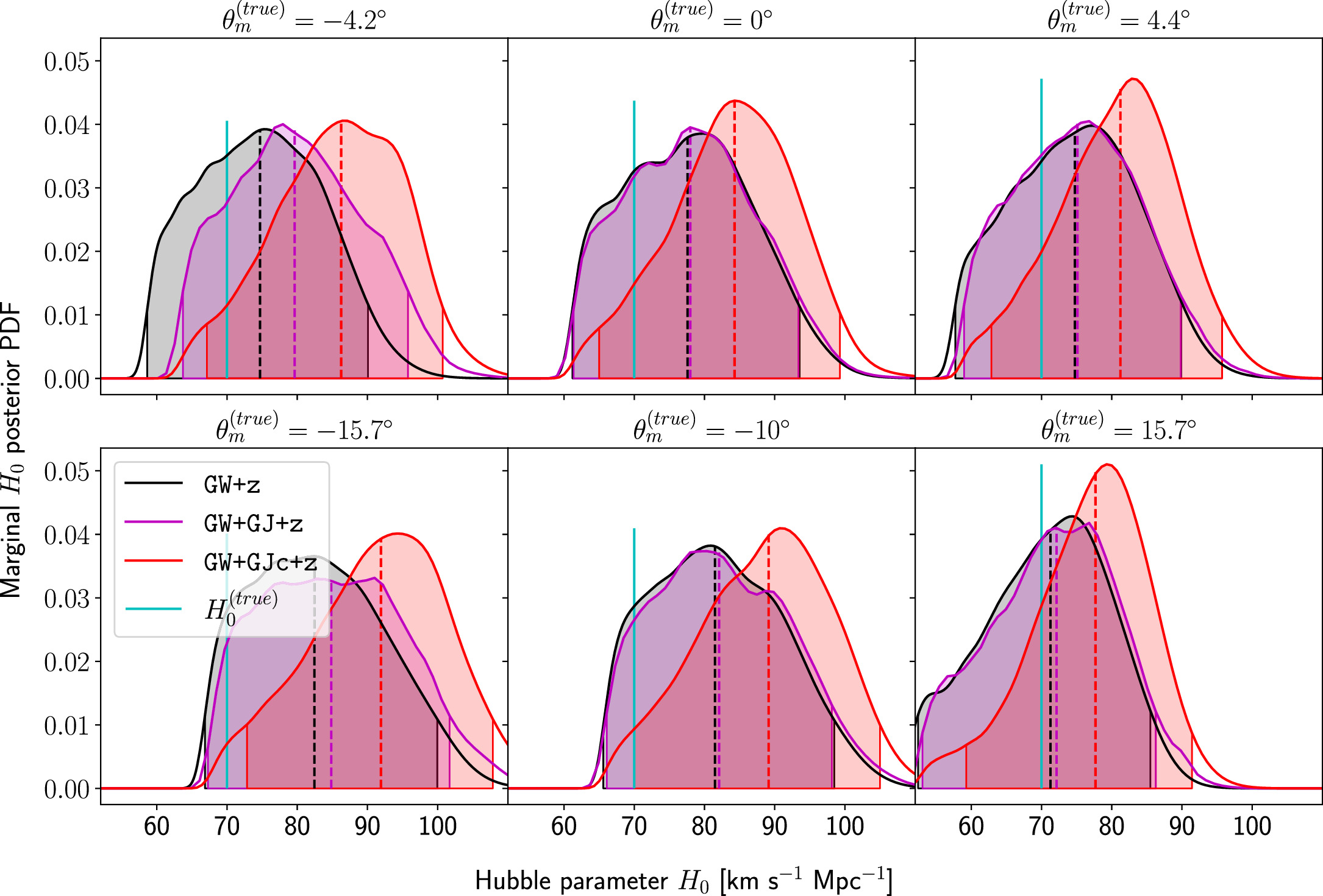
Figure B1. This figure shows the marginal posterior probability density functions (PDFs) for H0 from the  data sets at
  in the case of the co-inference of (θm, H0), as discussed in Section 3.3. We present the same angles as in Figure 5, and the median and 2.5th–97.5th percentiles of the marginal posterior are shown with a dashed line and colored regions (using the same color as for the PDF), respectively.
Download figure:
Standard image High-resolution image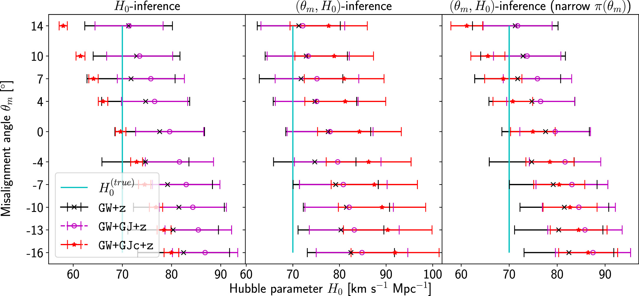
Figure B2. This figure shows the median and standard deviation (with error bars) for the (marginal) H0 posteriors, considering all available  data sets at
  . The leftmost set shows the behavior for standard inference with H0 and assuming
  and complements Figures 3 and 4. The set in the middle refers to the co-inference of (θm, H0), as discussed in Section 3.3, with a
  prior for θm (complementing Figures 5 and B1). The set on the right also considers the co-inference of (θm, H0) but with a narrower prior of
  for θm, which complements Figure B4.
Download figure:
Standard image High-resolution imageTable B5 and Figure B3 show the statistics corresponding to the marginalized H0 posteriors from the bias-mitigating inference of all aligned ( ) data sets. Based on these, one can judge if this method can recover zero misalignment angle for the aligned GW and EM data sets.
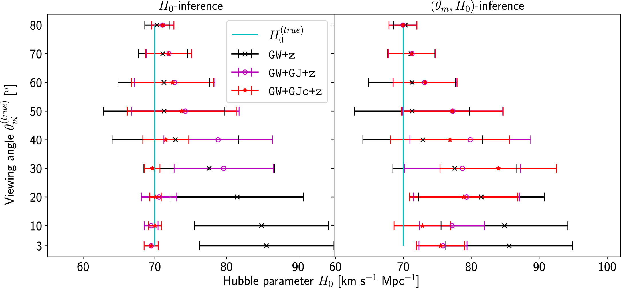
Figure B3. This figure shows the median and standard deviation (with error bars) for the (marginal) H0 posteriors, considering all available  data sets. The left column shows the behavior for standard inference with H0, which assumes
  . The right column refers to the co-inference of (θm, H0), as discussed in Section 3.3, with a
  prior for θm.
Download figure:
Standard image High-resolution image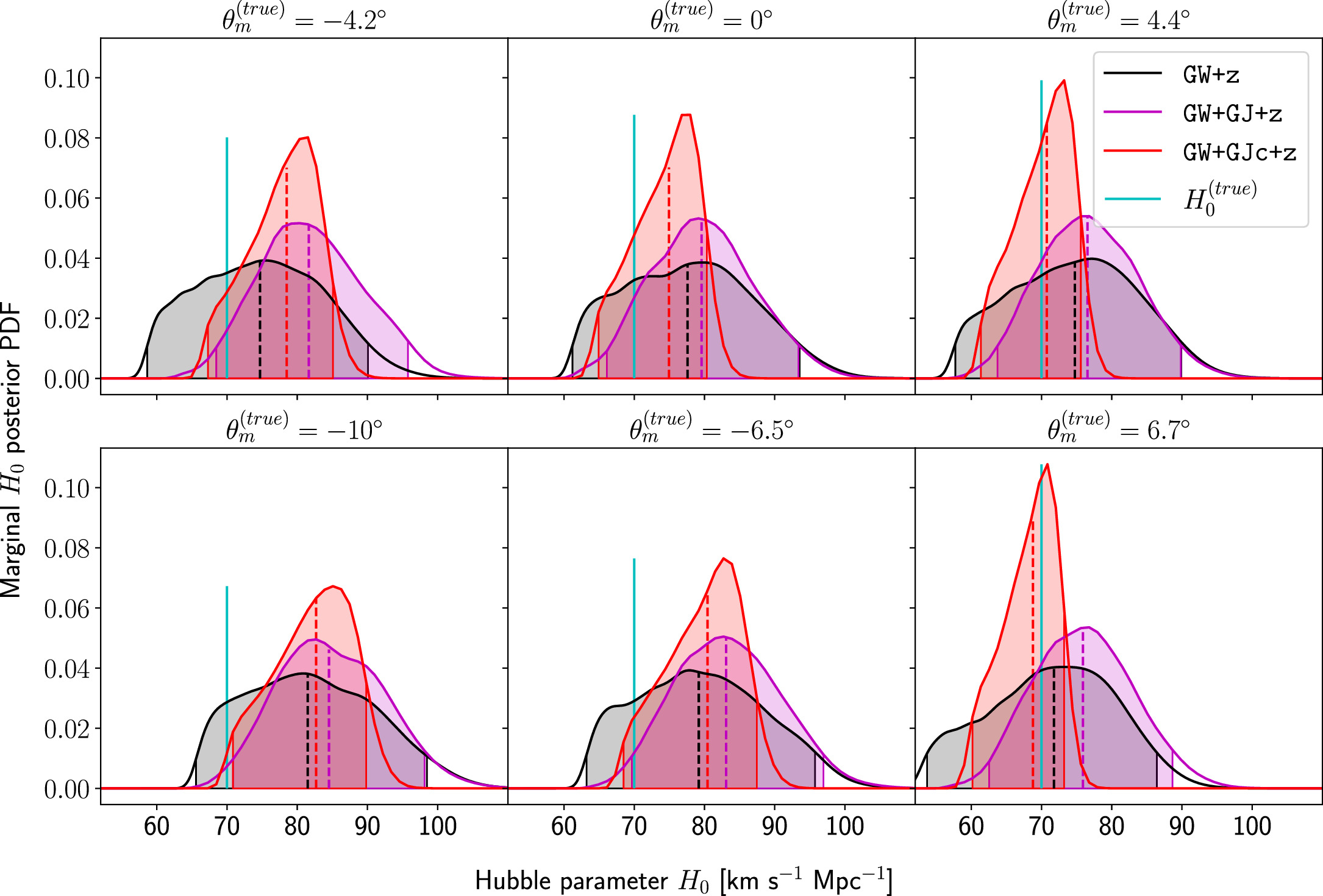
Figure B4. This figure shows the marginal posterior PDFs for H0 from the  data sets at
  in the case of the co-inference of (θm, H0) using the narrower prior
  for θm, as discussed in Section 3.3. We present the data for
  , −6
, −65, −4
2, 0°, 4
2, 6
7}, and the median and 2.5th–97.5th percentiles of the marginal posterior are shown with a dashed line and colored regions (using the same color as for the PDF), respectively.
Download figure:
Standard image High-resolution imageTable B5. Inferred Hubble Parameter for Different Inference Scenarios with Zero Misalignment Angle in the Datasets, but using Co-inference of the Misalignment Angle and H0

| H0 (Median, 2.5th–97.5th Percentiles) | |||
|---|---|---|---|---|
| GW+GJ+z | GW+PLJ+z | GW+GJc+z | GW+PLJc+z | |
| 3° |

|

|

|

|
| 10° |

|

|

|

|
| 20° |

|

|

|

|
| 30° |

|

|

|

|
| 40° |

|

|

|

|
| 50° |

|

|

|

|
| 60° |

|

|

|

|
| 70° |

|

|

|

|
| 80° |

|

|

|

|
Note. This table lists the median and 2.5th–97.5th percentiles of the marginal posterior results for the Hubble parameter from the  data sets in the case of the co-inference of (θm, H0), as discussed in Section 3.3.
Download table as: ASCIITypeset image
The presentations in Figures B2 and B3 should allow for an easy extraction of ![$\mathrm{med}\left[{H}_{0}\right]$](https://content.cld.iop.org/journals/2041-8205/977/2/L45/revision1/apjlad8dd1ieqn390.gif) and
and  and therefore
  and
and  . For comparison with the uniformed prior for the misalignment angle, in Figure B4 and the third column of Figure B2, we present statistics for the same analysis as in Figure B1; when we employ a narrower prior on the value of θm, in particular, we use
  .
.
Footnotes
- 5
- 6
- 7
The jet is a polar outflow from both poles; consequently, the scenario with θvi > π/2 is an equivalent scenario indistinguishable from θvi < π/2, and it is therefore sufficient to consider the range θvi ∈ [0, π/2]. Consequently, when we want to compare this with the system inclination, we also need to project the former into this range using the map
 ; see B. P. Abbott et al. (2017c). The line-of-sight misalignment θm is a lower bound to the full misalignment . The rest of the misalignment will show itself as a difference in the orientations of the jet and GW systems on the sky, which we do not pursue further in this work.
 - 8
This is justified by the theoretical expectation that the majority of mergers observed in the future will have moderate inclinations (B. F. Schutz 2011), similar to GW170817.
- 9
Furthermore, they use a fixed bias for all events, while we are trying to quantify the actual bias through modeling choices, which can vary from event to event and also bias in different directions; we need to point out this difference more clearly.
- 10
Note that there might be severe peculiar velocity systematics at short distances, such that high precision might not imply high accuracy, but this is a bias that we are not considering here.
- 11
- 12
This is chosen in order to remove the statistical fluctuation due to variation in the noise seed and demonstrate the systematic bias due to EM modeling misalignment.
- 13