Abstract
We study the linear stability of a planar interface separating two fluids in relative motion, focusing on conditions appropriate for the boundaries of relativistic jets. The jet is magnetically dominated, whereas the ambient wind is gas-pressure-dominated. We derive the most general form of the dispersion relation and provide an analytical approximation of its solution for an ambient sound speed much smaller than the jet Alfvén speed vA, as appropriate for realistic systems. The stability properties are chiefly determined by the angle ψ between the wavevector and the jet magnetic field. For ψ = π/2, magnetic tension plays no role, and our solution resembles the one of a gas-pressure-dominated jet. Here, only sub-Alfvénic jets are unstable ( , where v is the shear velocity and θ the angle between the velocity and the wavevector). For ψ = 0, the free energy in the velocity shear needs to overcome the magnetic tension, and only super-Alfvénic jets are unstable (
![$1\lt {M}_{e}\lt \sqrt{{(1+{{\rm{\Gamma }}}_{w}^{2})/[1+({v}_{{\rm{A}}}/c)}^{2}{{\rm{\Gamma }}}_{w}^{2}]}$](https://content.cld.iop.org/journals/2041-8205/951/2/L23/revision1/apjlacdfcfieqn2.gif) , with Γw the wind adiabatic index). Our results have important implications for the propagation and emission of relativistic magnetized jets.
, with Γw the wind adiabatic index). Our results have important implications for the propagation and emission of relativistic magnetized jets.
Original content from this work may be used under the terms of the Creative Commons Attribution 4.0 licence. Any further distribution of this work must maintain attribution to the author(s) and the title of the work, journal citation and DOI.
1. Introduction
The Kelvin–Helmholtz instability (KHI; Von Helmholtz & Monats 1868; Lord Kelvin 1871)—at the interface of two fluids in relative motion—is one of the most ubiquitous and well-studied instabilities in the universe. Since the pioneering works of Chandrasekhar (1961), the linear theory of the KHI has been investigated under a variety of conditions (Blumen et al. 1975; Blandford & Pringle 1976; Turland & Scheuer 1976; Ferrari et al. 1978, 1980; Pu & Kivelson 1983; Kivelson & Zu-Yin1984; Sharma & Chhajlani 1998; Bodo et al. 2004, 2013,2016, 2019; Osmanov et al. 2008; Prajapati & Chhajlani 2010; Hamlin & Newman 2013; Sobacchi & Lyubarsky 2018; Berlok & Pfrommer 2019; Pimentel & Lora-Clavijo 2019; Rowan 2019), depending on whether the relative motion is nonrelativistic or ultrarelativistic, whether the two fluids have comparable or different properties (respectively, “symmetric” or “asymmetric” configuration), whether the flow is incompressible or compressible, and whether or not the fluids are magnetized.
The boundaries of relativistic astrophysical jets may be prone to the KHI, given the relative (generally, ultrarelativistic) shear velocity between the jet and the ambient medium (hereafter, the “wind”). In jet boundaries with flow-aligned magnetic fields, KH vortices can wrap up the field lines onto themselves, leading to particle acceleration via reconnection (Rowan 2019; Sironi et al. 2021). Particles pre-energized by reconnection (e.g., Sironi & Spitkovsky 2014; Zhang et al. 2021; Sironi 2022) can then experience shear-driven acceleration (Rieger 2019; Wang et al. 2021, 2023)—i.e., particles scatter in between regions that move toward each other because of the velocity shear, akin to the Fermi process in converging flows (Fermi 1949). The KHI may then constitute a fundamental building block for our understanding of the origin of radio-emitting electrons in limb-brightened relativistic jets (e.g., in Cygnus A—Boccardi et al. 2016; and in M87—Walker et al. 2018), and for the prospects of shear-driven acceleration at jet boundaries in generating ultra-high-energy cosmic rays.
A study of the KHI in this context needs to account for the unique properties of the boundaries of relativistic jets. First, the relative motion between the jet and the wind can be ultrarelativistic; second, while the wind is likely gas-pressure-dominated, relativistic jets are believed to be magnetically dominated (Blandford & Znajek 1977), i.e., an asymmetric configuration. The linear stability properties of the KHI in this regime (of relativistic, asymmetric, magnetized flows) are still unexplored. In this letter, we derive the most general form of the dispersion relation for the KHI at the interface between a magnetized relativistic jet and a gas-pressure-dominated wind. We also provide an analytical approximation of its solution for wind sound speeds much smaller than the jet Alfvén speed, as appropriate for realistic astrophysical systems.
2. Setup
We consider a planar vortex sheet interface in the x–z plane at y = 0, as shown in Figure 1. The jet (y > 0) is cold and magnetized, with field
B
0j
= (B0x
, 0, B0z
) lying in the x–z plane and Alfvén speed vA. The ambient wind (y < 0) is gas-pressure-supported (with sound speed csw) and has a vanishing magnetic field. We use the subscript “j” for the jet and “w” for the wind. We solve the system in the jet rest frame, where the wind moves with velocity  . We adopt Gaussian units such that c = 4 π = 1 and define all velocities in units of c.
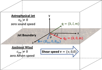
Figure 1. A 3D schematic diagram of the boundary of the relativistic jet. The boundary (gray color) is located in the x − z plane. Above and below the boundary are the magnetically dominated cold jet and the unmagnetized gas-pressure-supported ambient wind, respectively. q ∥ is the projection of the wavevector q onto the boundary. The jet is at rest and the wind has a relative shear speed of v . The magnetic field in the jet is B . θ is the angle between q ∥ and v , while ψ is the angle between B and q ∥.
Download figure:
Standard image High-resolution imageWe describe the flow with the equations of relativistic magnetohydrodynamics (RMHDs; e.g., Mignone et al. 2018; Rowan 2019):


supplemented with the divergence constraints

Here, ρ, ρe
,
J
,
v
, γ,
B
,
E
, w, and p are the rest-mass density, charge density, current density, fluid velocity, Lorentz factor ( ), magnetic field, electric field, gas enthalpy density, and pressure, respectively. For an ideal gas with adiabatic index Γ, the enthalpy can be written as w = ρ + Γp/(Γ − 1).
We assume a cold and magnetically dominated jet, with Alfvén speed  , where
and the jet enthalpy density is w0j ≈ ρ0j for a cold jet. The wind has negligible magnetic field and is gas-pressure-supported, with sound speed (Mignone et al. 2018)
where w0w is the wind enthalpy density. From pressure balance across the interface,
where Γw is the wind adiabatic index.
3. Dispersion Relation
The dispersion relation of surface waves at the interface can be found from the dispersion relations of body waves in both the jet and the ambient wind, together with the displacement matching at the interface. The dispersion relations of body waves in each of the two fluids can be found by linearizing Equation (1), such that the perturbed variables take the form φ ≈ φ0 + φ1, where φ0 and φ1 are the background and the first-order perturbed variables respectively. The perturbed electric field in the jet is E 1 = − v 1 × B 0j in the ideal MHD limit, 4 where v 1 is the perturbed velocity in the jet frame.
In the jet, we consider perturbed variables φ1 of the form φ1 ∝ ei(
q
·
x
−ω
t), where
q
= (k, lj
, m) is the complex wavevector and ω is the complex angular frequency, both defined in the jet rest frame. Note that  implies that the amplitude of the wave grows exponentially, i.e., an instability. We define the angle θ between the projection of the wavevector onto the x–z plane and the direction
  of the shear flow velocity such that

Similarly, we define the angle ψ between the wavevector projection onto the x − z plane and the jet magnetic field such that

For a magnetized cold jet, the dispersion relation of its body waves describes magnetosonic waves in the cold plasma limit:

In the wind, we consider perturbed variables φ1 of the form  , where
  is the complex wavevector and
  is the complex angular frequency, both defined in the wind rest frame. For an unmagnetized wind, the dispersion relation of its body waves reduces to the one of sound waves,
  . By Lorentz transformations of
  and
and  , we obtain

Since lj and lw are Lorentz invariant, by solving Equations (8) and (9) for lj and lw , respectively, we can construct a Lorentz-invariant ratio:
An independent way of obtaining lw /lj is to simultaneously solve the linearized RMHD equation, Equation (1), together with the first-order pressure balance equation,

and the displacement matching condition at the interface,

yielding
Using Equation (5), we can eliminate w0w /w0j from Equation (13) and, finally, the dispersion relation for the surface wave at the interface can be obtained by equating Equation (10) and the square of Equation (13):
By introducing the following notations,

Equation (14) can be rewritten as (Sobacchi & Lyubarsky 2018; Rowan 2019)
The dispersion relation in Equation (16) holds for arbitrary values of csw, vA, v,  , and
, and  , subject only to the assumptions of a cold jet and an unmagnetized wind.
Since Equation (16) is a sextic equation in ϕ, it has a total of six (generally, complex) roots. However, not all of them may be acceptable. First, not all of the solutions will satisfy Equation (13), since we have introduced spurious roots when squaring it. Also, by the Sommerfeld radiation condition (Sommerfeld 1912), only outgoing waves should be retained. This requires  and
and  . The expressions for lw
and lj
can be obtained from the derivation of Equation (13), so the Sommerfeld condition can be expressed as
. The expressions for lw
and lj
can be obtained from the derivation of Equation (13), so the Sommerfeld condition can be expressed as
4. Analytical Approximation
Since in general a sextic equation has no algebraic roots (Abel 1826), only approximate solutions of ϕ in Equation (16) can be obtained. We first note that the parameters in Equation (15) are chosen such that for a realistic wind with csw ≪ vA, we have ≪ 1, whereas the other parameters do not depend on csw. We then expand ϕ as a power series of
of the form ϕ ≈ c0 + c1
+ c2
2, where c0, c1, and c2 are constant with respect to
and terms higher than
2 are ignored. Substituting this into Equation (16) and comparing coefficients of various powers of
on both sides, we can find an approximate solution for all six roots of Equation (16). If we define an effective Mach number,

 , and recognize that
  , then the approximate roots that correspond to the unstable modes can be written as


where

We find that the first-order term Λ±
generally provides a good approximation of the numerical solution for ϕ. However, the second-order term (which we write explicitly in Appendix B) is required for identifying the physical solutions that satisfy Equation (13) and the Sommerfeld condition. At zeroth order in
, the real part of the solution (i.e., the phase speed of unstable modes) is ϕ = Me
, or equivalently ω/k = v, i.e., unstable modes are purely growing in the wind frame.
In Figures 2 and 3, we compare the numerical solution (left column) of Equation (16) with our analytical approximation (right column). We fix csw = 0.005 and consider vA = 0.2 and 0.8, so the assumption csw/vA ≪ 1 of our analytical approximation is well satisfied. The analytical solution for  displayed in the figures only employs the first-order terms (as discussed above, we also use the second-order terms to check the Sommerfeld constraint), yet it provides an excellent approximation of the numerical results, apart from Me
= 1. For Me
= 1, the first-order term Λ± of our analytical approximation diverges. We discuss below this special case.
displayed in the figures only employs the first-order terms (as discussed above, we also use the second-order terms to check the Sommerfeld constraint), yet it provides an excellent approximation of the numerical results, apart from Me
= 1. For Me
= 1, the first-order term Λ± of our analytical approximation diverges. We discuss below this special case.
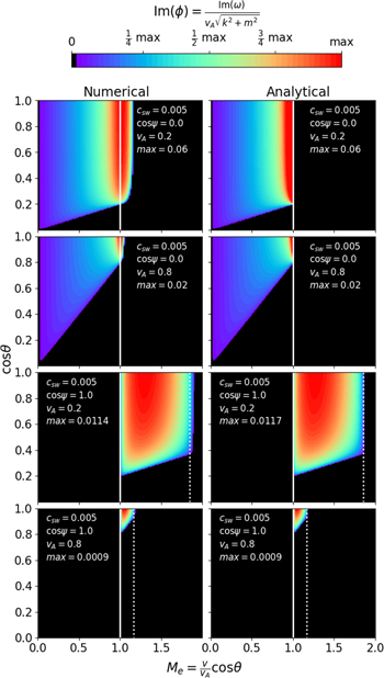
Figure 2. Dependence of the instability growth rate  on θ and Me
, for two choices of vA and two choices of
on θ and Me
, for two choices of vA and two choices of  , as indicated in the plots. The left and right columns represent the numerical and analytical solutions, respectively. For
  , the maximum growth rate of the analytical solution is capped at its numerical counterpart to avoid the divergence at Me
= 1. In all the panels,
, the maximum growth rate of the analytical solution is capped at its numerical counterpart to avoid the divergence at Me
= 1. In all the panels,  is then normalized to its maximum value, which is quoted in the panels themselves. The vertical dotted lines show the analytical upper bound on Me
when
is then normalized to its maximum value, which is quoted in the panels themselves. The vertical dotted lines show the analytical upper bound on Me
when  ; see Equation (26). The vertical solid white lines indicate Me
= 1.
; see Equation (26). The vertical solid white lines indicate Me
= 1.
Download figure:
Standard image High-resolution image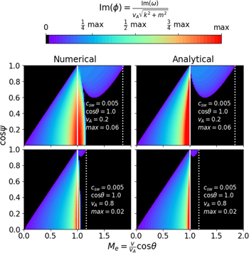
Figure 3. Dependence of the instability growth rate  on ψ and Me
, for two choices of vA as indicated in the plots. We fix
on ψ and Me
, for two choices of vA as indicated in the plots. We fix  . See the caption to Figure 2 for further details.
Download figure:
Standard image High-resolution imageOur analytical approximation allows us to determine the range of Me where the system is unstable. If λ in Equation (22) is imaginary, then also Λ± has a nonzero imaginary part. We then find the values of Me that satisfy λ2 = 0 and obtain the following unstable bounds: for Me < 1,
whereas for Me > 1,
where
Note that the condition  is equivalent to the obvious requirement v < 1. The condition
  in Equation (23) can be equivalently cast as
  , which has a simple interpretation. The system is unstable if the projection of the shear velocity onto the direction of
q
∥ (which we defined as the projection of the wavevector
q
on the x − z plane; see Figure 1) is larger than the projection of the Alfvén speed onto the same direction. In other words, the shear is able to overcome magnetic tension.
, which has a simple interpretation. The system is unstable if the projection of the shear velocity onto the direction of
q
∥ (which we defined as the projection of the wavevector
q
on the x − z plane; see Figure 1) is larger than the projection of the Alfvén speed onto the same direction. In other words, the shear is able to overcome magnetic tension.
Equations (23) and (24) fully characterize the instability boundaries in Figures 2 and 3. In particular, the vertical white dotted lines in the figures illustrate the upper bound in Equation (24) for the special case  , which yields
It follows that the unstable range at Me > 1 shrinks for vA → 1, but never disappears as long as vA < 1.
4.1. The Special Case Me = 1
In the case Me = 1, our analytical approximation diverges.
The singular case Me = 1 can be solved by expanding ϕ with a Puiseux series (Wall 2004; Wolfram Research 2020). Among the six approximate solutions of ϕ at Me = 1, the only unstable one is

where
In Appendix A, we demonstrate that this analytical approximation for the special case Me = 1 is in good agreement with the numerical solution.
Equation (27) allows us to identify the range of Me
(near unity) where the diverging growth rate in Equation (19) should rather be replaced by Equation (27). By equating the imaginary parts of  in Equation (19) and
  in Equation (27), and solving for Me
, we can obtain the upper bound
in Equation (27), and solving for Me
, we can obtain the upper bound  for Equation (19) such that
  for
for ![${M}_{e}\in [0,{M}_{e}^{* }]$](https://content.cld.iop.org/journals/2041-8205/951/2/L23/revision1/apjlacdfcfieqn36.gif) . We expect
. We expect  to be close to unity, so we assume Me
= 1 in μ and λ for Λ+ of Equation (19). The resulting expression for
to be close to unity, so we assume Me
= 1 in μ and λ for Λ+ of Equation (19). The resulting expression for  can then be written as

where we require < 33/221/5
ξ−1/2 for real
 .
.
4.2. Maximum Growth Rate
The results presented so far retain the explicit dependence on the angle θ between the projected wavevector
q
∥ and the flow velocity
v
, and on the angle ψ between
q
∥ and the magnetic field
B
(see Figure 1). In practice, for a given Mach number M = v/vA and a fixed magnetic field orientation (e.g., with respect to the shear direction), one can determine the maximum growth rate, irrespective of the specific value of θ at which it is attained. This is presented in Figure 4, where we show the peak growth rate as a function of M and  , where we define

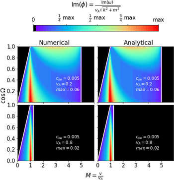
Figure 4. Dependence of the maximum instability growth rate  on
on  and M ≡ v/vA, for two choices of vA, as indicated in the plots. The maximum value of
  is taken across all values of
 ![$\cos \theta \in [0,1]$](https://content.cld.iop.org/journals/2041-8205/951/2/L23/revision1/apjlacdfcfieqn44.gif) for each
for each  pair. The left and right columns represent the numerical and analytical solutions, respectively. In all the panels,
  is then normalized to its maximum value, which is quoted in the panels themselves. The white lines indicate
  and M = 1/vA.
Download figure:
Standard image High-resolution imageThe plot shows that, for most magnetic field orientations, the peak growth rate is achieved at M ∼ 1. The exception is the case of fields nearly aligned with the shear velocity, where magnetic tension pushes the unstable region to higher M. The region of stability in the upper left corner is delimited by  (the white line), which comes from the instability condition
  in Equation (23). The range of unstable Mach numbers extends up to M < 1/vA (the vertical white line), which simply corresponds to the requirement v < 1.
5. Comparison to the Hydrodynamic Case
When the unstable mode propagates perpendicular to the magnetic field ( ), we expect magnetic tension to have no effect, and the solution should resemble the hydrodynamic asymmetric case discussed by Blandford & Pringle (1976). We demonstrate this by choosing a different parameterization in Equation (16), similar to the one of Equation (2) in Blandford & Pringle (1976), i.e.,
where  is the total enthalpy of the jet, namely the sum of the gas enthalpy w0j
and the magnetic enthalpy:
is the total enthalpy of the jet, namely the sum of the gas enthalpy w0j
and the magnetic enthalpy:

Then the dispersion relation Equation (16) can be equivalently written as
which, by setting  , is exactly the same as Equation (1) in Blandford & Pringle (1976), where both the jet and the wind were assumed to be unmagnetized. We conclude that, even though our jet is magnetized, in the case
  , the instability behaves similarly to the case of a hydrodynamic jet. Here, the magnetic field provides pressure, but not tension.
6. Discussion and Conclusions
We have studied the linear stability properties of the KHI for relativistic, asymmetric, magnetized flows, with a focus on conditions appropriate for the interface between a magnetized relativistic jet and a gas-pressure-dominated wind. We derive the most general form of the dispersion relation and provide an analytical approximation of its solution for = csw/vA ≪ 1. The stability properties are chiefly determined by the angle ψ between the jet magnetic field and the wavevector projection onto the jet/wind interface. For ψ = π/2, magnetic tension plays no role, and our solution resembles the one of a gas-pressure-dominated jet. Here, only sub-Alfvénic jets are unstable (
 , as long as v < 1). For ψ = 0, the velocity shear needs to overcome the magnetic tension, and only super-Alfvénic jets are unstable (
 ). At zeroth order in
 , the phase speed of unstable modes is ω/k = v in the jet frame, i.e., they are purely growing in the wind frame.
Our analytical results are valuable for both theoretical and observational studies. They can be easily incorporated into global MHD simulations of jet launching and propagation, to identify KH-unstable surfaces (Chatterjee et al. 2020; Sironi et al. 2021; Wong et al. 2021). On the observational side, claims have been made that the KHI is observed along active galactic nucleus (AGN) jets, based on the geometry of the outflow (Lobanov & Zensus 2001; Issaoun et al. 2022). Our formulae can place this claim on solid grounds, if estimates of the field strength and orientation and of the flow velocities are available. Besides AGNs, our results have implications for other jetted sources, such as, but not limited to, gamma-ray bursts, tidal disruption events, X-ray binaries, and pulsar wind nebulae.
We conclude with a few caveats. First, the plane-parallel approach we employed is applicable only if the jet/wind interface is much narrower than the jet radius (for studies of surface instabilities in force-free cylindrical jets, see, e.g., Bodo et al. 2013, 2016, 2019; Sobacchi & Lyubarsky 2018). Second, our local description implicitly assumes that the flow properties do not change as the KHI grows. Third, we have assumed the jet plasma to be cold, and the surrounding medium to be unmagnetized. These assumptions will be relaxed in a future work.
Acknowledgments
We are grateful to R. Narayan for many inspiring discussions and collaboration on this topic. We would like to thank G. Bodo for many useful discussions and suggestions. L.S. acknowledges support from the Cottrell Scholars Award and the DoE Early Career Award DE-SC0023015. L.S and J.D. acknowledge support from NSF AST-2108201, NSF PHY-1903412, and NSF PHY-2206609. J.D. is supported by a Joint Columbia University/Flatiron Research Fellowship, and research at the Flatiron Institute is supported by the Simons Foundation.
Appendix A: Analytical Approximation for Me = 1
For the singular case Me
= 1, our analytical solutions take the form of the first-order Puiseux series. Here, we compare the analytical and numerical solutions. In Figures 5 and 6, we plot the instability growth rate for Me
= 1, comparing analytical and numerical solutions. We choose the same parameters as in the figures of the main paper, namely csw = 0.005 and vA = 0.2 or 0.8. We fix  for Figure 5 and
  for Figure 6. We use solid and dashed lines to represent numerical and analytical solutions, respectively. The figures show that our analytical solutions in Puiseux series provide a good approximation to the numerical ones across the entire range of
  (for Figure 5) and
  (for Figure 6).
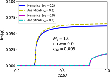
Figure 5. Dependence of the instability growth rate Im (ϕ) on  for two choices of vA and a fixed value of
  in the singular case Me
= 1. The solid lines represent the numerical solutions, while the dashed lines represent the analytical solutions obtained by Puiseux series expansion in the main text.
in the singular case Me
= 1. The solid lines represent the numerical solutions, while the dashed lines represent the analytical solutions obtained by Puiseux series expansion in the main text.
Download figure:
Standard image High-resolution image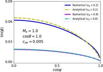
Figure 6. Dependence of the instability growth rate Im (ϕ) on  for two choices of vA and a fixed value of
  in the singular case Me
= 1. The solid lines represent the numerical solutions, while the dashed lines represent the analytical solutions obtained by Puiseux series expansion in the main text.
in the singular case Me
= 1. The solid lines represent the numerical solutions, while the dashed lines represent the analytical solutions obtained by Puiseux series expansion in the main text.
Download figure:
Standard image High-resolution imageAppendix B: The Second-order Terms
In the main body of the paper, we have looked for an analytical approximation of the form ϕ ≈ c0 + c1
+ c2
2, where c0, c1, and c2 are constant with respect to
and terms higher than
2 are ignored. For the unstable solutions, we find that the first-order term Λ±
generally provides a good approximation of the numerical solution. However, the second-order term Σ±
2 is required for identifying the physical solutions that satisfy the Sommerfeld condition. The explicit expression for Σ± is

Footnotes
- 4
Resistive effects are likely important in the nonlinear stages (Sironi et al. 2021), but not for the linear analysis presented here.