Abstract
Time-dependent energy spectra of galactic cosmic rays (GCRs) carry fundamental information regarding their origin and propagation. When observed at the Earth, these spectra are significantly affected by the solar wind and the embedded solar magnetic field that permeates the heliosphere, changing significantly over an 11 yr solar cycle. Energy spectra of GCRs measured during different epochs of solar activity provide crucial information for a thorough understanding of solar and heliospheric phenomena. The PAMELA experiment collected data for almost 10 years (2006 June 15–2016 January 23), including the minimum phase of solar cycle 23 and the maximum phase of solar cycle 24. In this paper, we present new spectra for helium nuclei measured by the PAMELA instrument from 2010 January to 2014 September over a three-Carrington-rotation time basis. These data are compared to the PAMELA spectra measured during the previous solar minimum, providing a picture of the time dependence of the helium-nuclei fluxes over a nearly full solar cycle. Time and rigidity dependencies are observed in the proton-to-helium flux ratios. The force-field approximation of the solar modulation was used to relate these dependencies to the shapes of the local interstellar proton and helium-nuclei spectra.
Original content from this work may be used under the terms of the Creative Commons Attribution 4.0 licence. Any further distribution of this work must maintain attribution to the author(s) and the title of the work, journal citation and DOI.
1. Introduction
Since the end of the last century, there has been a flury of new measurements of the energy spectra and composition of the cosmic radiation with significant improvement in the statistical precision and reduction in the systematic uncertainties (for a review, see Boezio et al. 2020). These measurements have provided new insights and breakthroughs in the investigation of the origin and propagation of galactic cosmic rays (GCRs), e.g., Blasi (2014), Amato & Blasi (2018). Particularly significant are the measurements on protons and helium nuclei (e.g., Adriani et al. 2011; Aguilar et al. 2014; Adriani et al. 2019; An et al. 2019), the most abundant components of GCRs. However, the near totality of these measurements were obtained deep inside the heliosphere where the influence of the solar wind is especially important.
The solar wind is a plasma of ionized gas emitted by the Sun corona. The solar wind, whose existence was fully realized by Parker in 1958 (Parker 1958), expands at supersonic speed into space, creating the heliosphere, a region of space over which our Sun’s influence dominates. Since the solar wind is coupled with the Sun corona, it carries the solar magnetic field present in the corona out into the solar system, creating the heliospheric magnetic field (HMF). It has long been known that solar activity has an 11 yr periodicity (Usoskin 2017) over which the solar wind pattern and intensity of the HMF vary significantly. During a period of minimum activity, the Sun’s global magnetic field has its simplest form, while it tends to assume a chaotic structure near maximum activity. Additionally, the solar magnetic field undergoes a polarity reversal during solar maximum, resulting in a 22 yr cycle for the polarity of the HMF.
The energy spectra of the cosmic rays as measured at Earth is affected by their interaction with the turbulent solar wind and the embedded magnetic field characterizing the heliosphere. When they arrive at Earth the characteristics of the heliosphere are imprinted in their energy spectra (e.g., Heber 2013; Potgieter 2013). Therefore, a precise understanding of the transport of GCRs in the heliosphere is required to fully exploit the precise information provided by the experimental measurements (e.g., Potgieter et al. 2014, 2015). Conversely, precise measurements of the cosmic-ray energy spectra down to fractions of GeV and their time dependence over a solar cycle provide unique insights on the fundamental properties of the solar wind and magnetic field turbulence in the heliosphere, the modulation of GCRs, and the characteristics of solar activity.
The PAMELA satellite-born experiment was launched from the baikonur cosmodrome in Kazakhstan on 2016 June 15. Then, for nearly a solar cycle, from the 23rd solar minimum through the maximum of solar cycle 24, PAMELA made high-precision measurements of the charged component of cosmic radiation. The PAMELA collaboration has already published several papers on GCR solar modulation: protons (Adriani et al. 2013; Martucci et al. 2018), electrons and positrons (Adriani et al. 2015, 2016b) and, most recently, the time-dependent helium spectra during the 23rd solar minimum (2006 July–2019 December; Marcelli et al. 2020). In this paper, the measurement of the helium-nuclei component is extended up to the end of the 24th solar maximum (2014 September). The new energy spectra were evaluated on a three-Carrington-rotation time (≃81 days) basis from 2010 January to 2014 September, from Carrington numbers 2092–2154 according to the official numbering. No isotopic separation was done in this analysis; the fluxes are the sum of 3He and 4He components.
These fluxes are combined with the previous published data to present the time dependence of the helium-nuclei spectrum over a nearly complete solar cycle.
Additionally, for the same time period, the proton-to-helium flux ratios are presented as a function of time and rigidity to highlight dependencies, possibly due to the different particle masses and shapes of the local interstellar spectra (Tomassetti et al. 2018; Corti et al. 2019; Ngobeni et al. 2020). Finally, a simplified approach to solar modulation, the force-field approximation (Gleeson & Axford 1968), is used to relate these dependencies to the shapes of the local interstellar proton and helium-nuclei spectra.
2. Instrument and Data Analysis
After its launch, the PAMELA experiment was almost continuously taking data until 2016 January. The experiment was located on board the Resurs-DK1 Russian satellite, placed by a Soyuz rocket at a highly inclined (70°) elliptical orbit between 350 and 600 km height that changed into a circular one of 580 km in 2010 September. The satellite quasi-polar orbit allowed the PAMELA instrument to sample low cutoff-rigidity orbital regions for a considerable amount of time, making it suitable for low-energy particle studies. The apparatus consisted of a combination of detectors that provided information for particle identification and precise rigidity (R) measurements. These detectors were: a time-of-flight system, a magnetic spectrometer, an anti-coincidence system, an electromagnetic imaging calorimeter, a shower tail catcher scintillator, and a neutron detector. Detailed information about the instrument and its performance can be found in Picozza et al. (2007) and Adriani et al. (2014, 2017).
The statistics of selected events were found to decrease over time. This effect was mainly due to the sudden, random failure of a few front-end chips in the tracking system and it became particularly significant after 2009. Therefore, in this analysis, the helium fluxes were evaluated on a three-Carrington-rotation time basis. In the time period covered in this analysis, the solar activity was at its maximum and characterized by many solar events. Most of these events produced high-energy particles capable of reaching Earth and, consequently, the PAMELA detector. Similar to the approach adopted in the analysis of the time dependence of GCR protons (Martucci et al. 2018), the time periods corresponding to these solar events, according to the measurements of the low-energy (>60 MeV) proton channel of GOES-15 28 , were not included in this work.
The analysis procedure used in this work was identical to the one used to determine the time dependence of the helium-nuclei fluxes over the solar minimum period presented and discussed in Marcelli et al. (2020). The absolute helium-nuclei fluxes Φ(K) in kinetic energy (K) were obtained as follows:

where N(K) is the unfolded count distribution of selected events, (K) the product of the single-selection efficiencies, G(K) the geometrical factor, LT the live-time, and ΔK the width of the energy interval. The total selection efficiency was ∼ 22% at the beginning of 2011, decreasing to ∼12% toward the end of 2014. This was mainly driven by the aforementioned condition of the tracking system. The geometrical factor for selected helium nuclei above 2 GV is 17.5 cm2 sr.
No isotopic separation (possible only up to ≈1.4 GeV n−1 Adriani et al. 2016a) was performed in this analysis. For the conversion from rigidity to kinetic energy, all helium-nuclei events were treated as 4He.
3. Results
The resulting energy spectra are presented in Figure 1, left panel, which shows the time evolution of measured differential helium fluxes as a function of kinetic energy, from 2010 January (violet curve) to 2014 September (red curve). The right panel shows the helium flux ratio with respect to the flux measured in 2010 January. The effect of solar modulation is clearly visible in the energy region below few GeV n−1 where it causes the flux to decrease significantly and subsequently modifies the spectral shape with increasing solar activity.
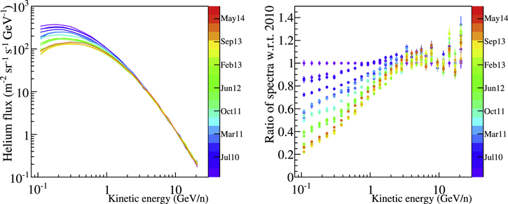
Figure 1. Left panel: the evolution of the helium energy spectrum as intensities approached the period of maximum solar activity, from 2010 January (violet) to 2014 September (red). Right panel: the ratio of the measured spectra with respect to the spectrum of 2010 January. The color code is the same as the right panel.
Download figure:
Standard image High-resolution imageThe flux intensity measured at the energy interval 95–123 MeV n−1 dropped by about 70% from 2010 January to 2014 September, while the flux intensity at 337–427 MeV n−1 decreased about 50% during the same time interval. At energies above ∼15 GeV n−1, the solar modulation effect is assumed negligible with respect to the experimental uncertainties.
Figure 2 shows a comparison between two PAMELA and AMS-02 helium fluxes measured during Carrington rotation numbers 2110-2112 and 2143-2145. The published AMS-02 fluxes (Aguilar et al. 2018) were averaged over three Carrington rotations to match the PAMELA time periods. An excellent agreement between the two sets of measurements can be noticed in the overlapping rigidity region as shown in the bottom panel by the constant fits on the ratios between PAMELA and AMS-02 measured fluxes.
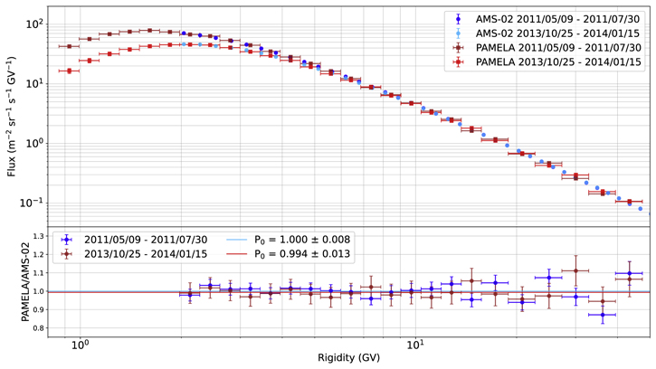
Figure 2. Top: PAMELA helium spectra measured in 2011 and late 2013 compared with the corresponding AMS-02 measurements (Aguilar et al. 2018), as indicated in the legend. The AMS-02 fluxes were averaged over three Carrington rotations. Bottom: the ratios between PAMELA and AMS-02 fluxes. A constant fit was performed on the ratios and the results (P0) are shown in the legend.
Download figure:
Standard image High-resolution imageThe time dependencies of protons and helium nuclei were analyzed by measuring the proton-to-helium flux ratio as a function of time and rigidity. Figure 3 shows this ratio for five rigidity intervals for increased solar activity, this work, and for the preceding solar minimum period (Marcelli et al. 2020). Since the quantity measured by the magnetic spectrometer is rigidity, this approach allows a more precise estimation of the ratios considering that systematic uncertainties, related to the same instrumental effects, cancel out. The residual systematic uncertainty includes only the errors due to the efficiency estimation. The error bars in Figure 3 are the quadratic sum of the statistical errors and this residual systematic error. To reduce the statistical fluctuation for the data points after 2009, a weighted average over nine months was performed, while the data points relative to the solar minimum are shown with the original time basis, described in Marcelli et al. (2020). Each rigidity interval of the two data sets (until 2009 and from 2010) were fit with a constant (P0) function, whose fitted lines and values are shown in Figure 3. There is a clear evidence of a decrease in time for the lowest rigidity intervals from minimum to maximum solar activity period. On the contrary, the higher rigidity intervals show hints of the opposite behavior as the ratios increase from minimum to maximum solar activity.
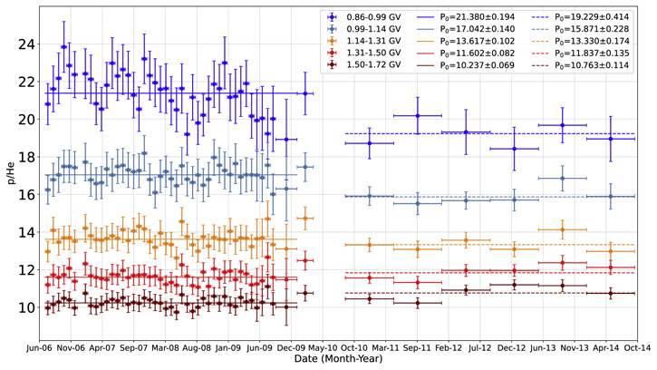
Figure 3. Time profiles of proton-to-helium ratio for the five rigidity intervals specified in the legend. The error bars are the quadratic sum of statistical and systematic errors. After 2009 the data points cover nine Carrington rotation time periods. The lines and P0 parameters resulting from the fit of a constant in each rigidity bin in the solar minimum (solid line) and maximum (dashed line) periods are also shown.
Download figure:
Standard image High-resolution imageFinally, Figure 4 shows the PAMELA proton over helium ratio for a wider rigidity range and normalized to the mean value of the ratio in the period from 2013 May to 2014 September, when the solar activity reached its maximum. To reduce the effect of the short-term cyclic variation in the solar minimum period, mainly visible in the lowest rigidity interval in Figure 3, a weighted average over a nine-month time basis was performed. The last point before 2010 corresponds to a weighted average over 10 months. The AMS-02 data (Aguilar et al. 2018), normalized over the same solar maximum period, are also shown for the period after 2014 September, with the rigidity bins combined to better match those of PAMELA data. A clear time dependence is observed for the lowest rigidity bin (blue), which decreases from minimum to maximum solar activity period. Conversely, above about 1.5 GV (red and yellow) the proton-to-helium ratio shows an increase from 2006 to 2014 followed by a comparable decrease seen in the AMS-02 data. These time and rigidity dependencies can be related to effects caused by the solar modulation of protons and helium because of the difference in their mass-to-charge ratio and in the shape of their respective LIS. For an illustration of these modulation effects, see Ngobeni et al. 2020).
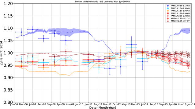
Figure 4. Time profile of the proton-to-helium ratio at the rigidity intervals listed in the legend, normalized to the mean value of the ratios in the solar maximum period from 2013 May to 2014 September. The error bars are the quadratic sum of statistical and systematic errors. A weighted average over 9 months (with the exception of the last point before 2010, which is a weighted average over 10 months) was performed to reduce statistical fluctuation and the effect of the short-term cyclic variation in the solar minimum period. The AMS-02 data (Aguilar et al. 2018), normalized over the same solar maximum period, are shown for the period after 2014 September. The dashed lines are the proton-to-helium ratios and their corresponding uncertainties, colored bands, derived using the force-field approximation for solar modulation as described in Section 4.
Download figure:
Standard image High-resolution imageA detailed theoretical modeling of the proton-to-helium flux ratio will be the topic of a future publication. In this work, a first analysis of the relevance of the LIS shapes for the features of this ratio was conducted using the force-field approximation for solar modulation.
4. Data Interpretation and Discussion
Assuming the force-field approximation, appropriate for GCR with kinetic energies above about 200 MeV/n, of the spherically symmetric model for solar modulation suggested by Gleeson & Axford (1968), the differential GCR intensity J(r, E, t) at a given distance r from the Sun, total energy E, and time t, is related to the time-independent interstellar GCR intensity J( ∞ , E) through the equation:

where E0 is the rest energy (mass) of the particle and Φ = ∣Z∣e ϕ a parameter that can be interpreted as the energy loss experienced by the cosmic-ray particle when approaching the Earth from infinity. Therefore, the time dependence of the GCR fluxes due to solar modulation is reproduced by the time dependence of the solar modulation parameter ϕ. Consequently, if ϕ is known, the LIS can be extrapolated from the modulated spectrum using Equation (2).
In this work, the solar modulation parameters were obtained with the following procedure (for more details, see Marcelli 2021). Following Gleeson & Axford (1968), two sets of curves, shown in Figure 5, were obtained by plotting the measured proton and helium-nuclei fluxes divided by rigidity squared, i.e., J/R2, as a function of the kinetic energy divided by the particle charge, i.e., K/Ze. As can be seen in Figure 5, above 0.5 GV, these curves have a similar shape but are displaced along the abscissa. These displacements represent the time-dependent change, Δϕ, in the solar modulation parameter (ϕ = ϕ0 + Δϕ). From these curves, the Δϕ were obtained for both particle species and, as expected (Gleeson & Axford 1968), inside the experimental uncertainties were found identical and comparable to the variations of the solar modulation parameter determined by Koldobskiy et al. (2019) using neutron monitor, AMS-02 and PAMELA data. Subsequently, a set of LIS, one for each measured modulated spectrum, was estimated assuming a ϕ0 value of 300 MV and, then, merged into a single spectrum with a weighted average procedure. The flux values of this resulting LIS were combined with the Voyager 1 data (Stone et al. 2013; Cummings et al. 2016) at lower energies. Then, the value of ϕ0 was increased at steps of 10 MV and for each step a new combined LIS was obtained. The LIS that had the smoothest spectrum data 29 provided the best value for ϕ0, which was found to be 500 MV both for protons and helium nuclei. Consequently, the best LIS for the two-particle species were also obtained. Finally, these LIS were modulated with the estimated modulation parameters for the period 2006–2017 June and the proton-to-helium flux ratios of the resulting modulated fluxes were calculated. For the period 2014 October–2017 June the solar modulation parameters estimated by Koldobskiy et al. (2019) were used. These ratios are shown in Figure 4 as dashed curves along with the propagated uncertainties (sum of statistical and systematic errors) of the measured fluxes shown as colored bands.
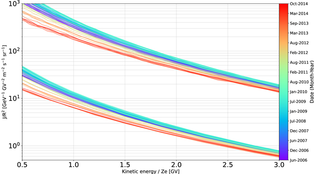
Figure 5. Proton (top set of lines) and helium-nuclei (lower lines) fluxes (J) measured by the PAMELA experiment from 2006 June (violet) to 2014 September (red) divided by rigidity squared vs. kinetic energy divided by the charge (Ze). The displacements along the abscissa are similar between the two species and they are attributed to the varying with time of the solar modulation parameter.
Download figure:
Standard image High-resolution imageConsidering the significant approximation of the force-field approach, it is worth noting that the calculated proton-to-helium flux ratios qualitatively reproduce the time and rigidity dependencies observed with the experimental data of both PAMELA (until 2014 September) and AMS-02 (after 2014 September).
Since the force-field approximation assumes the same modulation parameter for different particle species, this result would indicate that, in the rigidity range of these measurements, the observed time variation of the proton-to-helium flux ratios are dominated by the shapes of the proton and helium-nuclei LIS, while the dependence of the diffusion tensor of the heliospheric transport equation on the particle mass-to-charge ratio would appear to play an increasing role at lower rigidities.
5. Conclusions
The PAMELA experiment observed GCR data for nearly a complete solar cycle from the minimum phase of solar cycle 23 to the maximum phase of solar cycle 24. In this work, we have presented new spectra for helium nuclei measured by the PAMELA instrument from 2010 January until 2014 September integrating the previously published data. These measurements allow a detailed study of the propagation of cosmic rays inside the heliosphere. Comparing the helium-nuclei fluxes to the proton fluxes, time and rigidity dependencies are clearly observed. A quantitative study, based on state-of-the-art models (e.g., Ngobeni et al. 2020) of these dependencies is underway and will be presented in a future publication. However, a simplified approach based on the force-field approximation of solar modulation was able to relate these dependencies to the shapes of the local interstellar proton and helium-nuclei spectra.
The results discussed in this paper will be available at the Cosmic Ray Data Base of the ASI Space Science Data Center (http://tools.asdc.asi.it/CosmicRays/chargedCosmicRays.jsp).
We acknowledge partial financial support from The Italian Space Agency (ASI). We also acknowledge support from Deutsches Zentrum fur Luft-und Raumfahrt (DLR), The Swedish National Space Board, The Swedish Research Council, The Russian Space Agency (Roscosmos), Russian Science Foundation No-20-72-10170, RFBR and Russian ministry of science. R.M. acknowledges partial financial support from the INFN grant “giovani,” project ASMDM.
Footnotes
- 28
- 29
The smoothness of each spectrum was obtained by dividing the standard deviation of the differences between consecutive flux values by the mean of these differences. Then the smoothest spectrum was the one with the minimum value for the smoothness.