Abstract
Protons detected by the PAMELA experiment in the period 2006–2014 have been analyzed in the energy range between 0.40 and 50 GV to explore possible periodicities besides the well known solar undecennial modulation. An unexpected clear and regular feature has been found at rigidities below 15 GV, with a quasi-periodicity of ∼450 days. A possible Jovian origin of this periodicity has been investigated in different ways. The results seem to favor a small but not negligible contribution to cosmic rays from the Jovian magnetosphere, even if other explanations cannot be excluded.
1. Introduction
The dominant and most important timescale in cosmic rays, related to solar activity, is the 11-year cycle (Tobias 2002). This quasi-periodicity is translated into the galactic cosmic-ray (GCR) intensities widely recorded by the network of ground stations since the 1950s (Lockwood & Webber 1967). Later, a 22-year cycle was discovered, linked to the reversal of the heliospheric magnetic field (HMF) taking place during each period of large solar activity Webber & Lockwood (1988). There are also indications of GCR periodicities of 50–65 years, 90–130 years, and also for a periodicity of more than 200 years (Potgieter 2013).
Moreover, short periodicities (like 25–27-day and 1-day cycles) have been observed in many GCR data, related to the rotation of the Sun and of the Earth respectively (Alania et al. 2011; Schwachheim 1960). How these periodicities are generated and how they could be explained through the not fully established Parker heliospheric coefficients (Strong et al. 2007) is still a matter of study. More recently, new data have been provided by the high-precision measurements of GCRs performed by the satellite experiment PAMELA in a wide range of energy in the period 2006–2015, covering the end phase of the twenty-third solar cycle and almost the whole twenty-fourth cycle (Adriani et al. 2013, 2015, 2016).
2. PAMELA Detector
The PAMELA apparatus consists of a combination of detectors capable of identifying particles up to oxygen and giving information on charge, mass, rigidity, and velocity from a few tens of MeV up to 1 TeV. The instrument is built around a permanent magnet with a silicon microstrip tracker, providing charge and track deflection information. A scintillator system provides trigger, time-of-flight, and additional charge information. A silicon–tungsten calorimeter is used to perform general hadron–lepton separation. An anti-coincidence system of plastic scintillators allows the rejection of spurious events in the off-line phase. A comprehensive description of the instrument, the mission profile, the scientific objectives and the results achieved during the PAMELA 10-year operation in space, can be found in Adriani et al. (2014).
3. The Analysis
The PAMELA proton data have been analyzed in three different rigidity ranges: 0.4–0.65 GV, 0.65–15 GV, and 15–50 GV to explore possible unexpected periodicities. Following the methods described in Adriani et al. (2013) for a clear identification of low energy GCR protons, daily-averaged intensities have been calculated for the overall period 2006 July 9th–2014 August 31st.
To ensure a clean galactic sample, contamination of solar particles from solar flares has been avoided, discarding bunches of data taken during major solar particle events (a list of these events is reported in Adriani et al. 2017). Other short-term effects on GCRs, like Forbush decreases, caused by coronal mass ejections passing through Earth, have been removed, even if their impact on the proton intensities appears negligible for most events.
In Figure 1, the daily proton intensity time profile J(t) for the aforementioned rigidity intervals is shown. The large gaps in the data (between 2010 and 2011) are due to periods in which the instrument was not fully operational. Different phases of the solar cycle are visible in the shape of the intensity profiles: from 2006 to January 2009 the twenty-third solar cycle comes to an end and the proton flux slowly increases due to a stable condition of the heliosphere, as already described in Adriani et al. (2013). After 2010, the activity of the twenty-fourth cycle gradually rises and the proton flux decreases accordingly.
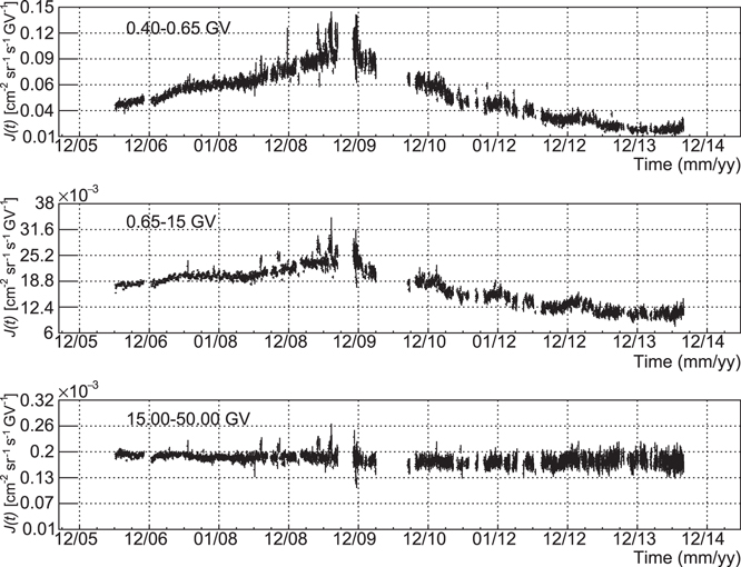
Figure 1. Daily proton intensity J(t) as a function of time for the rigidity intervals described in the text. Different phases of solar cycles 23 and 24 are clearly observable. The channel 15–50 GV is almost unaffected by solar modulation.
Download figure:
Standard image High-resolution imageIn addition to the expected overall trend, almost disappearing after 15 GV, the low rigidity profiles present some small and regular peaks, mostly during the descending phase of the modulation cycle. In order to highlight these peaks, a fit of the proton flux J(t) has been performed to try to disentangle possible high frequencies in the proton data from the well known undecennial modulation. Two distinct third-degree polynomials, in the form  , one for the data during the ascending phase J1(t) and another for the descending one J2(t), have been used. This approach ensures a statistically good compromise between the number of free parameters and precision. The fluctuations ξ1(t) and ξ2(t) between the experimental data of the two solar phases and the results of the respective fits f3(t) were evaluated without taking into account the period around the maximum:

These fluctuations are presented together, as ξ(t), for each of the two most significant rigidity channels in the first two panels of Figure 3. A quasi-periodic oscillation appears, more evident after 2010 December. For comparison, the same technique has been applied to the data of the Apatity Neutron Monitor (http://www.nmdb.eu/nest/search.php/); the results, reported in the third panel of Figure 3, show a periodicity that seems to coincide with the observed one by PAMELA. To try to explore the origin of this quasi-periodicity, a raw periodgram (95% Kolmogorov–Smirnov confidence level) of the first two rigidity spectra, 0.4–0.65 GV and 0.65–15 GV, has been carried out. The results are presented in the fifth panel of Figure 3. Peaks appear around 580, 450, 370, 320, and 230 days. The 580-day periodicity is possibly linked to an ∼600-day periodicity reported in Valdés-Galicia et al. (1996), which could be associated with fluctuations in the southern coronal hole area and in large active regions. The seasonal ∼370-day cosmic-ray variation is caused by the Earth’s rotation (Forbush 1954). The 230-day peak was also found in El-Borie et al. (2011) as a 0.7-year periodicity during the A > 0 solar cycle (1992–2000). The last periodicity, ∼450 days, was already described in Valdés-Galicia et al. (1996) as a possible 1.2-year periodicity but its origin is not reported.
The nature of the ∼450-day periodicity could be related to quasi biennial oscillations or QBOs (Vecchio et al. 2012; Laurenza et al. 2012). QBOs have been detected as a prominent scale of variability in GCRs, but they could just be more an effect of superposition of other periodic/quasi-periodic processes and not stochastic perturbations. Higher QBOs have been observed during solar maxima with respect to solar minima (Bazilevskaya et al. 2015); this could explain a higher signal in the descending phase of PAMELA proton data (see Figure 1) and could be related to different drift effects in different polarities of the HMF. In the past, numerous periodicities between 0.5 and 4 years have been correlated to QBOs (Kato et al. 2003; Rybák et al. 2001; Kudela et al. 2002, 2010; Benevolenskaya (1998) and it is very difficult to disentangle their effects from others.
In this work, a different hypothesis is proposed for the 450-day periodicity as a study case: a Jovian origin, more exotic but largely proposed in the past. It is well known that the planet Jupiter possesses a very intense magnetosphere due to the combination between its strong magnetic field, about 104 times larger than that of the Earth, and the weakness of the solar wind at 5 au. Evidence that Jupiter could generate high-energy particles has been shown for electrons (Teegarden et al. 1974; Simpson et al. 1974), and more recent studies revealed that the impulsive and quasi-periodic bursts observed in Jupiter’s duskside magnetosphere also contain protons and helium nuclei in the range 0.7–10 MeV/nucleon (Zhang et al. 1995).
Moreover, an indication that acceleration mechanisms can operate in magnetospheric environments has been found on Earth, where trapped particles are shown to be accelerated to relativistic energies by local acceleration acting in the heart of the Van Allen radiation belts (Reeves et al. 2013).
The hypothesis that some cosmic rays observed at Earth can be generated in the Jovian magnetosphere, at least up to energies of the order of few gigaelectron volts, and then injected in the interplanetary space along the magnetic-field force lines, has been discussed in the past (Pizzella & Venditti 1973; Pizzella 1975; Mitra et al. 1983) using the observations of ground stations. With a synodic period of 398.88 days, the Jovian assumption could be somehow related to the ∼450-day periodicity found in PAMELA data. In fact, having also regard to the uncertainty bar in the periodgram of Figure 3, the peak around 450 days could be compatible with a value close to 400 days, but the limited data-taking is not sufficient to clearly resolve them. It is worth noting that if some protons arrive guided by the interplanetary magnetic-field (IMF) lines connecting Jupiter to Earth, larger fluxes are expected at certain angles. If an angle ΦEJ is defined as the Earth longitude in a reference system with the center in the Sun and corotating with Jupiter, as shown in Figure 2, it is possible to associate with every daily proton intensity measured by PAMELA the respective value of the geometrical angle ΦEJ, which can be obtained from http://pds-rings.seti.org/tools/ephem2_jup.html.
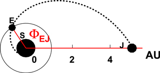
Figure 2. Schematic view of the Earth–Sun–Jupiter system with the IMF line connecting Jupiter with Earth (dashed line). The angle ΦEJ describes the purely geometrical angle between both planets.
Download figure:
Standard image High-resolution imageThe ΦEJ profile as a function of time is shown in Figure 3, fourth panel.
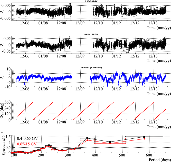
Figure 3. Fluctuations ξ(t) as a function of time are presented together for the two most significant rigidity channels of PAMELA (first two panels). A quasi-periodic oscillation appears before and after the gap, more visible starting from 2010 December. In the third panel, the same periodicity seems to be also present in the Apatity neutron monitor data. The fourth panel represents the time profile of the angle ΦEJ between Earth and Jupiter. The last panel shows the results of the periodgram performed on PAMELA data in the first two rigidity channels (0.4–0.65 GV and 0.65–15 GV).
Download figure:
Standard image High-resolution imageRecent descriptions, based on satellite data, give an IMF with spiral lines of force, but with a precise behavior that depends on the radial gradients of the magnetic field itself. It is found that the favored angle ΦEJ of the IMF lines connecting Earth and Jupiter is less than 180°:140° in Khabarova & Obridko (2012), 117° in Behannon (1978), or 150°/160° in Mitra et al. (1983).
Therefore, we followed an approach that takes into account these results.
The detrended daily proton averages, ξ(t), obtained through Equation (1), have been distributed in two samples: (a) protons associated with angles ΦEJ ≤ 180° and (b) protons associated with angles ΦEJ > 180°. If some protons arrive from Jupiter, a higher number of protons is expected in sector (a) with respect to sector (b), due to the Archimedean configuration of the Parker spiral originating from Sun Parker & Jokipii (1976).
Each of the two samples, (a) and (b), has been further separated in two sections, according to whether the protons were collected during the ascending phase of the solar modulation cycle or the descending phase:
- 1.a1 (ascending, ΦEJ ≤ 180°) from 2006 July 9 to 2009 July 9.
- 2.b1 (ascending, ΦEJ > 180°) from 2006 July 9 to 2009 July 9.
- 3.a2 (descending, ΦEJ ≤ 180°) from 2010 July 9 to 2014 August 31.
- 4.b2 (descending, ΦEJ > 180°) from 2010 July 9 to 2014 August 31.
After that, the average of each sample, ηa(1, 2) and ηb(1, 2), has been evaluated, together with its standard deviation, having verified that the distributions are normal.
Then, a variable Dj(j = 1, 2) is introduced for each couple ηaj(j = 1, 2) and ηbj(j = 1, 2) with the respective standard deviation:

The results are given in the Table 1 for the three rigidity channels.
Table 1. D and σtotal in Units of Proton/(cm2 sr s GV), the Excess of Proton Flux and S/N = D/σtotal are Represented
| Rigidity | Solar | D | σtotal | Excess | S/N | χ2/ndf | χ2/ndf |
|---|---|---|---|---|---|---|---|
| Interval (GV) | Phase | % | 0°–180° | 180°–360° | |||
| 0.4–0.65 | total | 0.000609 | 0.000052 | 4.3 | 11.7 | 0.97 | 0.98 |
| 0.4–0.65 | ascending | 0.000462 | 0.000067 | 2.6 | 6.9 | 0.77 | 0.74 |
| 0.4–0.65 | descending | 0.00073 | 0.000076 | 7.4 | 9.6 | 0.98 | 1.4 |
| 0.65–15 | total | 0.005948 | 0.00060 | 2.5 | 9.9 | 1.35 | 0.70 |
| 0.65–15 | ascending | 0.002056 | 0.00074 | 0.72 | 2.8 | 0.81 | 0.93 |
| 0.65–15 | descending | 0.00925 | 0.00091 | 4.8 | 10.2 | 1.1 | 0.97 |
| 15–50 | total | 0.00000172 | 0.00000041 | 0.96 | 4.2 | 2.0 | 1.7 |
| 15–50 | ascending | 0.00000137 | 0.00000042 | 0.74 | 3.3 | 0.99 | 1.4 |
| 15–50 | descending | 0.00000203 | 0.00000069 | 1.2 | 2.9 | 1.4 | 1.0 |
Note. The last two columns show the χ2/ndf calculated for Gaussian fits for the categories (a) and (b) in the text. We remark that all D values are positive and have large S/Ns.
Download table as: ASCIITypeset image
The same procedure has been followed also after summing a1 and b1 and a2 and b2, i.e., taking into account the entire period of data collection. The results appear in Table 1, labeled as Total.
For a uniform distribution of the protons along the Earth orbit, a value of D = 0, within errors, is expected. D results are always positive with a very large signal-to-noise ratio (S/N = D/σtotal) for each phase and each energy interval. The excess of protons in sector (a) with respect to those in sector (b) is evident, especially for the two lowest energy ranges.
If this excess was all due to Jupiter, the contribution to the GCR should be about 4.3% for the rigidity channel 0.4–0.65 GV, and 2.5% for the channel 0.65–15 GV. It is worth considering that, if part of the protons arrived along the IMF lines from Jupiter, larger fluxes should be expected at certain values of the angle ΦEJ. To also explore this behavior, each value of the fluctuations ξ, obtained through Equation (1), has been plotted as a function of the angle ΦEJ instead of the time (like in Figure 3). The resulting angular distribution is depicted in Figure 4 for the three rigidity channels, both for the ascending (left panel) and the descending (right panel) phases of the proton intensities. It is seen that there is an increase of GCR protons for both the phases when the angle ΦEJ lies between 60° and 200° with a maximum around 100°. The peak disappears almost entirely in the interval 15–50 GV.
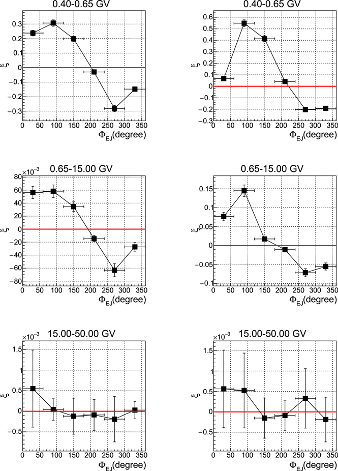
Figure 4. Distribution of the fluctuations ξ as a function of the relative positions of Earth and Jupiter, ΦEJ, for the rigidity channels 0.4–0.65 GV, 0.65–15 GV, and 15–50 GV. The left panel refers to the ascending phase, while the right panel refers to the descending one. A maximum around 100° is observed in the first two channels.
Download figure:
Standard image High-resolution image4. Discussion and Conclusions
It is worth noting that the precise PAMELA measurements, to our knowledge, are the first detected in space-borne experiments, exploring large periodicities in GCR intensities and also providing rigidity information. The results obtained in this work are in good agreement with the previous results reported in Mitra et al. (1983) and Pizzella & Venditti (1973), obtained with ground-based detectors. The difference with respect to Parker, who found an angle ΦEJ ∼ 216°, may be attributed to the IMF configuration considered in the classical calculation, that more recent experiments found to be much more complicated than the one proposed in the past (Khabarova & Obridko 2011, 2012; Behannon 1978). It should also be noted that the previous angular results were explained in Nagashima & Tatsuoka (1984) and Swinson (1974) as a possible effect due to anisotropies linked to the solar cycle. The results shown in this paper could favor the idea that the Jupiter magnetosphere might be a source of a small but not negligible fraction of protons measured at 1 au, accelerating particles by mechanisms like interaction with the solar wind Krimigis et al. (1981). If this is the right interpretation, we can venture out to conclude that magnetospheres of astrophysical systems (say, Jupiter, Pulsars, …) are possible sources of cosmic rays.
We acknowledge partial financial support from The Italian Space Agency (ASI) under the program “Programma PAMELA—attività scientifica di analisi dati in fase E.” We also acknowledge support from Deutsches Zentrum fur Luft- und Raumfahrt (DLR), The Swedish National Space Board, The Swedish Research Council, The Russian Space Agency (Roscosmos), and the Russian Science Foundation.