Abstract
We present five far- and near-ultraviolet spectra of the Type II plateau supernova, SN 2022acko, obtained 5, 6, 7, 19, and 21 days after explosion, all observed with the Hubble Space Telescope/Space Telescope Imaging Spectrograph. The first three epochs are earlier than any Type II plateau supernova has been observed in the far-ultraviolet revealing unprecedented characteristics. These three spectra are dominated by strong lines, primarily from metals, which contrasts with the featureless early optical spectra. The flux decreases over the initial time series as the ejecta cool and line blanketing takes effect. We model this unique data set with the non–local thermodynamic equilibrium radiation transport code CMFGEN, finding a good match to the explosion of a low-mass red supergiant with energy Ekin = 6 × 1050 erg. With these models we identify, for the first time, the ions that dominate the early ultraviolet spectra. We present optical photometry and spectroscopy, showing that SN 2022acko has a peak absolute magnitude of V = − 15.4 mag and plateau length of ∼115 days. The spectra closely resemble those of SN 2005cs and SN 2012A. Using the combined optical and ultraviolet spectra, we report the fraction of flux as a function of bluest wavelength on days 5, 7, and 19. We create a spectral time-series of Type II supernovae in the ultraviolet, demonstrating the rapid decline of flux over the first few weeks of evolution. Future observations of Type II supernovae are required to map out the landscape of exploding red supergiants, with and without circumstellar material, which is best revealed in high-quality ultraviolet spectra.
Original content from this work may be used under the terms of the Creative Commons Attribution 4.0 licence. Any further distribution of this work must maintain attribution to the author(s) and the title of the work, journal citation and DOI.
1. Introduction
Hydrogen-rich supernovae, also known as Type II supernovae, are thought to come from stars with masses ≳8 M⊙ (e.g., Woosley & Weaver 1986). While massive stars and their supernova explosions play a fundamental role in the evolution of the universe, many details of their evolution are not understood. Observations at various wavelengths and over multiple epochs can probe different aspects of the supernova explosion (e.g., Fransson et al. 1984; Dessart & Hillier 2005; Jencson et al. 2019). While complete optical coverage is becoming more common, ultraviolet (UV) spectroscopy remains almost nonexistent.
Although the UV is not well studied, these wavelengths contain a wealth of information. In contrast to the nearly featureless early optical, the early UV, and in particular the far-UV (FUV; λ < 1700 Å) is full of metal features. These features can be used to determine the composition of the outer stellar envelope or circumstellar material (CSM; material lost just prior to explosion), the density and temperature of the outer layers of the ejecta, as well as interaction between any CSM and the supernova photons and/or ejecta (e.g., Panagia et al. 1980; Fransson et al. 1984, 1987; Dessart & Hillier 2005, 2022). Additionally, as current and future missions such as JWST and the Nancy Grace Roman Space Telescope focus on the infrared (IR), understanding the UV spectra of massive star supernovae is key for interpreting the early universe where UV photons from the first supernovae are redshifted into the IR.
This lack of UV spectroscopy is due to two competing challenges. First, UV emission in Type II supernovae is powered by the energy deposited in the hydrogen-rich envelope by the shock that fades rapidly as it cools (Pritchard et al. 2014). This effect is enhanced by the large number of iron absorption features that appear in the first few weeks after explosion and blend together to absorb most of the UV flux (Pun et al. 1995; Dessart et al. 2008; Gezari et al. 2008; Dessart & Hillier 2010). Although all UV spectra eventually show this evolution, the timing and speed of the damping appear to vary (see Section 5.2). Second, the UV can only be observed from space, and the instruments best suited for these observations, the Space Telescope Imaging Spectrograph (STIS) and the Cosmic Origins Spectrograph (COS), are on the Hubble Space Telescope (HST), whose scheduling is not designed for rapid target of opportunity (ToO) observations. Nevertheless, a limited number of disruptive ToOs are designated each year with a turnaround time of 2–5 days. Adding an additional barrier to early observations is the fact that every HST detector capable of UV observations, other than the STIS/CCD (which only covers near-UV (NUV) wavelengths), must pass a bright object screening so as not to damage the detector.
The only FUV observations of Type II supernovae taken earlier than the spectra presented in this paper are from the International Ultraviolet Explorer (IUE) and are of atypical Type II supernovae (1980 K; Pettini et al. 1982, 1987A; Cassatella & Fransson et al. 1987; Fransson et al. 1987; Pun et al. 1995). The earliest FUV spectrum of a noninteracting normal Type II supernova is SN 1999em, observed ∼12 days after explosion (Baron et al. 2000). In the NUV there are a handful of early spectroscopic observations (SN 2005cs: Brown et al. 2007; SN 2021yja: Vasylyev et al. 2022; SN 2020fqv: Tinyanont et al. 2022; SN 2022wsp: Vasylyev et al. 2023; SN 2005ay: Gal-Yam et al. 2008; SN 2013ej: Dhungana et al. 2016); however, these spectra are either low signal-to-noise ratio (S/N), observed over a week postexplosion, or suffer from significant reddening. While Gal-Yam et al. (2008) noted the similarity of the NUV features of supernovae observed with GALEX, despite the optical diversity, the sample is based on three supernovae taken more than a week after explosion and did not extend to the FUV. The putative uniformity of the NUV spectra of Type II supernovae differs from the diversity observed in stripped-envelope supernovae (Kwok et al. 2022). A larger sample with better time sampling and S/N is required to assess the true diversity of this wavelength range.
With the limited lifetime of HST and the dearth of UV observations, we proposed in Cycle 30 to gather early FUV spectra of a Type II supernova (PI: Bostroem; GO-17132). We limited our selection to the most common kind of Type II supernovae, those that display either a plateau (IIP-like) or linear decline (IIL-like) in their optical light curves after peak and a rapid drop onto the radioactive tail, ∼80–120 days after explosion (Valenti et al. 2016).
On 2022 December 6 (JD 2459919.59), the Distance Less than 40 Mpc (DLT40) survey (Tartaglia et al. 2018), discovered SN 2022acko in NGC 1300 (Lundquist et al. 2022). A day later we activated a disruptive ToO with HST to obtain STIS FUV and NUV spectra in a 3 day time series, with a final epoch about 2 weeks later. Our observations executed within 3 days of triggering, resulting in the first FUV observations of a Type IIP supernova within 1 week of explosion (see Section 2 for the definition of explosion epoch), significantly earlier than the spectrum of SN 1999em taken ∼12 days after explosion.
In this Letter we present our UV data set, using optical data to place SN 2022acko in the context of other Type II supernovae. We describe the HST triggering process in Section 2. In Section 3 we present photometric and spectroscopic observations. The optical light-curve and spectroscopic evolution are described in Section 4. Finally, we describe the UV spectra and modeling in Section 5 before presenting our conclusions in Section 6.
2. HST Trigger and Scheduling
Early FUV spectral sequences are rare and have not been obtained for a Type IIP supernova because they require a nearby object, discovered and characterized early, with low extinction, in a field without other bright objects. In this section we describe the process of discovering, vetting, and triggering SN 2022acko for early HST FUV and NUV observations. Figure 1 summarizes this process, with the first 3 days shown in detail in the top panel, from detection through scheduling, and the full sequence in the bottom panel.
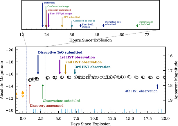
Figure 1. A timeline of events from discovery through the end of HST observations for SN 2022acko. The bottom panel shows the DLT40 open filter light curve (open circles) and the ATLAS limits (orange triangles). Key moments in the timeline are marked on the light curve. The epochs at which optical spectra were obtained are shown as light blue lines at the bottom of the figure. We observed at least one optical spectrum concurrent with each HST visit. The top panel shows the details of activities executed in the first 3 days after explosion to enable the triggering of HST. If any one of these events was unable to occur or was delayed, we would not have been able to observe SN 2022acko in the FUV.
Download figure:
Standard image High-resolution imageSN 2022acko was discovered by the DLT40 team (Tartaglia et al. 2018) on UT 2022 December 06 03:53:00 (JD 2459919.66; r = 16.54 mag). Within 15 minutes of discovery, it was confirmed with a second image, multiband imaging and spectroscopy were triggered, and the supernova was announced to the community via the Transient Name Server 29 (TNS; Lundquist et al. 2022). Using the automated infrastructure of the DLT40 survey (Yang et al. 2019), we immediately identified a deep ATLAS nondetection within 24 hr of discovery (JD 2459918.67, o > 19.1 mag; Smith et al. 2006; Tonry et al. 2018). Conservatively, we use this nondetection as the explosion epoch for the remainder of the Letter. The combination of the ATLAS nondetection and DLT40 discovery within 24 hr allowed us to trigger our Neil Gehrels Swift Observatory (Gehrels et al. 2004) GI proposal (PI: Dong; 1821204) to obtain 6 hr cadence UV and optical images of the supernova.
We received our first Swift photometry 14.5 hr after discovery, verifying that the supernova was UV bright and vetting the field for UV-bright sources using the uvw2 NUV filter image. SN 2022acko was classified as a Type II supernova 24 hr after discovery (Li et al. 2022), which was subsequently verified 1 hr later with another spectrum (Meza et al. 2022). We submitted the official HST disruptive ToO trigger 28 hr after the discovery of SN 2022acko. The bright object protection (BOP) review was completed 44 hr after discovery, and the ToO was scheduled to execute ∼2.5 days later.
The first three epochs were executed 5.2, 6.0, and 7.3 days after explosion (JD 2,459,923.87, 2,459,924.66, and 2,459,925.98), respectively. These constitute the earliest FUV observations of a Type IIP/L supernova to date and some of the earliest NUV observations. Scheduling constraints prevented our final epoch from being taken a week after the initial sequence, and we thus observed SN 2022acko 18.9 days after explosion (JD 2,459,937.53), completing our proposed sequence.
Unfortunately, the second epoch failed to acquire guide stars and only one FUV exposure was taken. We immediately notified the Space Telescope Science Institute (STScI) of the failure and were awarded an additional orbit. Due to the same scheduling constraints that limited the execution of the fourth epoch, the makeup epoch executed 20.7 days after explosion (JD 2,459,938.89). Given the expected low FUV flux, we devoted this epoch exclusively to the NUV.
3. Observations
We triggered high-cadence photometric and spectroscopic follow-up observations immediately following the discovery of SN 2022acko with both ground- and space-based instruments. Below we report on the facilities used and the data that were collected over this campaign.
3.1. Photometry
We obtained UBgVri-band photometry from the Las Cumbres Observatory’s network of 0.4 m, 1 m, and 2 m telescopes (Brown et al. 2013) through the Global Supernova Project (GSP) collaboration and BgVri-band and Open filter photometry from SkyNet’s network of 0.4 m PROMPT telescopes (Reichart et al. 2005) through the DLT40 collaboration. The multiband images from SkyNet are a new capability that enable the DLT40 collaboration to obtain very high-cadence coverage over the optical wavelength range. This is the first published light curve to utilize this new feature.
Las Cumbres Observatory images were bias corrected and flat fielded using BANZAI (McCully et al. 2018) then point-spread function photometry was performed in an IRAF-based pipeline (Valenti et al. 2016). The SkyNet images were processed and aperture photometry performed in a python-based pipeline for all color filters. UBV magnitudes are presented in Vega magnitudes while gri-band magnitudes are given in AB magnitudes. The Open filter SkyNet images were reduced with difference imaging using HOTPANTS (Becker 2015) prior to magnitudes being extracted and then calibrated to the r band. We supplement these observations with photometry downloaded from the ATLAS forced photometry service in the orange filter (Smith et al. 2006; Tonry et al. 2018).
UV and optical imaging was also obtained with the UVOT instrument (Roming et al. 2005) on Swift in the uvw2, uvm2, uvw1, u, b, and v filters. The rapid response of Swift provided key information on the UV brightness of SN 2022acko, essential for triggering HST, and caught the rarely seen NUV light-curve rise. Images were reduced with aperture photometry using the High-energy Astrophysics Software UVOT routines (HEASARC 2014) with the updated sensitivity of Breeveld et al. (2011). We used a 54 aperture set to encompass the full light of the supernova and a region near the supernova was selected and used to subtract the background. Photometry is automatically corrected for aperture and coincidence losses. The final UV images are upper limits only, as the supernova has faded below the background flux of the host galaxy. It is possible that more detections can be recovered with difference imaging when late-time templates are obtained. The late-time UV photometry is sensitive to contamination by the underlying host galaxy and therefore both the object and background aperture must be carefully selected. Experimenting with different aperture sizes and background locations, we find that this primarily affects the Swift UV limits.
3.2. Spectroscopy
We obtained ground-based optical spectra with the FLOYDS spectrograph on the Las Cumbres Observatory 2 m Faulkes Telescopes North and South (FTN and FTS; Brown et al. 2013) through the GSP collaboration.
Additional spectra were obtained with the Binospec spectrograph on the MMT (Fabricant et al. 2019), the Boller and Chivens (B&C) spectrograph 30 on the Bok Telescope, the Robert Stobie Spectrograph (RSS) on the Southern African Large Telescope (SALT; Smith et al. 2006), the Goodman Spectrograph on the Southern Astrophysical Research Telescope (SOAR; Clemens et al. 2004), Multi-Object Double Spectrograph (MODS; Pogge et al. 2010) on the Large Binocular Telescope (LBT; Hill 2010), and the Intermediate Dispersion Spectrograph (IDS) at the Isaac Newton Telescope (INT). Other spectra were downloaded directly from the TNS. A complete list of spectroscopic observations is given in Table 1 and shown in Figure 2.
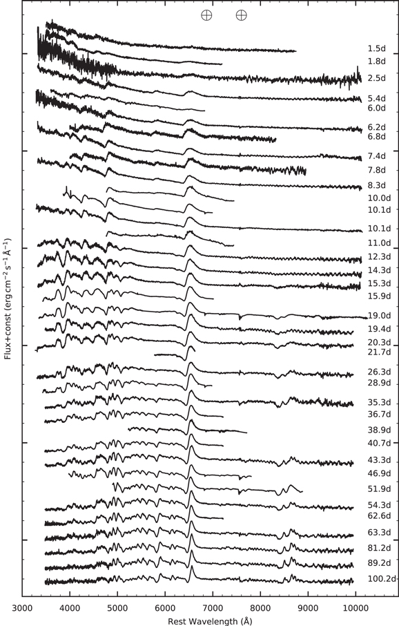
Figure 2. The spectroscopic evolution of SN 2022acko in the optical. The phase of each spectrum, relative to the date of last nondetection, is marked on the right. Telluric features are marked at the top of the figure. The spectra shown in this figure are available as the data behind the figure.(The data used to create this figure are available.)
Download figure:
Standard image High-resolution imageTable 1. Spectroscopic Observations of SN 2022acko
| Observer-frame | JD | Telescope | Instrument |
|---|---|---|---|
| Phase (days) | |||
| 1.5 | 2,459,920.17 | Lijiang-2.4 m | YFOSC |
| 1.8 | 2,459,920.47 | SALT | RSS |
| 2.5 | 2,459,921.17 | FTS | FLOYDS |
| 5.2 | 2,459,923.87 | HST | STIS |
| 5.4 | 2,459,924.10 | FTS | FLOYDS |
| 6.0 | 2,459,924.65 | Bok | B&C |
| 6.0 | 2,459,924.66 | HST | STIS |
| 6.2 | 2,459,924.90 | FTN | FLOYDS |
| 6.8 | 2,459,925.50 | INT | IDS |
| 7.3 | 2,459,925.98 | HST | STIS |
| 7.4 | 2,459,926.04 | FTS | FLOYDS |
| 7.8 | 2,459,926.50 | INT | IDS |
| 8.3 | 2,459,926.96 | FTS | FLOYDS |
| 10.0 | 2,459,928.72 | Bok | B&C |
| 10.1 | 2,459,928.73 | SOAR | Goodman |
| 10.1 | 2,459,928.75 | FTN | FLOYDS |
| 11.0 | 2,459,929.67 | Bok | B&C |
| 12.3 | 2,459,931.02 | FTS | FLOYDS |
| 14.3 | 2,459,932.92 | FTS | FLOYDS |
| 15.3 | 2,459,933.98 | FTS | FLOYDS |
| 15.9 | 2,459,934.61 | SOAR | Goodman |
| 18.9 | 2,459,937.54 | HST | STIS |
| 19.0 | 2,459,937.63 | LBT | MODS |
| 19.4 | 2,459,938.08 | FTS | FLOYDS |
| 20.3 | 2,459,938.99 | FTS | FLOYDS |
| 20.7 | 2,459,939.39 | HST | STIS |
| 21.7 | 2,459,940.42 | SALT | RSS |
| 28.9 | 2,459,944.97 | FTS | FLOYDS |
| 35.3 | 2,459,947.62 | SOAR | Goodman |
| 35.2 | 2,459,953.94 | FTS | FLOYDS |
| 36.7 | 2,459,955.40 | SALT | RSS |
| 38.9 | 2,459,957.60 | MMT | Binospec |
| 40.7 | 2,459,959.38 | SALT | RSS |
| 43.3 | 2,459,961.98 | FTS | FLOYDS |
| 46.9 | 2,459,965.58 | SOAR | Goodman |
| 51.9 | 2,459,970.56 | SOAR | Goodman |
| 54.3 | 2,459,972.95 | FTS | FLOYDS |
| 62.6 | 2,459,981.31 | SALT | RSS |
| 63.3 | 2,459,981.95 | FTS | FLOYDS |
| 81.2 | 2,459,999.90 | FTS | FLOYDS |
| 89.2 | 2,460,007.90 | FTS | FLOYDS |
| 100.2 | 2,460,018.90 | FTS | FLOYDS |
Download table as: ASCIITypeset image
Most spectroscopic observations were reduced with IRAF (B&C) or IRAF-based pipelines (FLOYDS: Valenti et al. 2014; MODS: Pogge 2019) using standard reduction techniques. RSS observations were reduced with a custom pipeline using the PySALT software package (Crawford et al. 2010), Binospec was reduced with a custom IDL pipeline (Kansky et al. 2019), IDS spectra were reduced with the custom python package IDSRED (Bravo 2023), and Goodman spectra were reduced with a custom python package. 31 All spectra were scaled to the Swift photometry and gri-band photometry using either a constant offset or linear fit.
3.3. HST UV Spectroscopic Observations
FUV and NUV spectra were obtained with HST/STIS 5.2, 6.0, 7.3, and 18.9 days after explosion. A final NUV spectrum was obtained with STIS on day 20.8. Observations were taken with the G140L and G230L gratings using the FUV- and NUV-MAMA detectors, respectively, with the 52″ × 02 slit. Exposure time, resolution, and wavelength range for these observations are given in Table 2. Reduced observations were downloaded from the Mikulski Archive for Space Telescopes (MAST). The data described here may be obtained from the MAST archive at doi:10.17909/gaze-k021.
Table 2. HST/STIS Observations of SN 2022acko
| Observer-frame Phase (day)s | JD | Grating | Exposure Time (s) | Resolving Power | Wavelength Range (Å) |
|---|---|---|---|---|---|
| 5.2 | 2,459,923.92459923.9 | G140L | 3000 | 1000 | 1150–1730 |
| 5.3 | 2,459,924.0 | G230L | 1500 | 500 | 1570–3180 |
| 6.0 | 2,459,924.7 | G140L | 2250 | 1000 | 1150–1730 |
| 7.3 | 2,459,926.0 | G140L | 1465 | 1000 | 1150–1730 |
| 7.3 | 2,459,926.0 | G230L | 440 | 500 | 1570–3180 |
| 18.9 | 2,459,937.6 | G140L | 6604 | 1000 | 1150–1730 |
| 19.0 | 2,459,937.7 | G230L | 757 | 500 | 1570–3180 |
| 20.8 | 2,459,939.4 | G230L | 2278 | 500 | 1570–3180 |
Download table as: ASCIITypeset image
4. Analysis
SN 2022acko exploded in a spiral arm of NGC 1300 (z = 0.00526; Springob et al. 2005), a well-studied nearby galaxy. Figure 3 32 shows the location of SN 2022acko in a star-forming region of NGC 1300, in a composite JWST, HST, Very Large Telescope (VLT)/Multi-Unit Spectroscopic Explorer (MUSE), and Atacama Large Millimeter/submillimeter Array (ALMA) image. For the analysis of SN 2022acko, we must first define the distance to the host galaxy as well as galactic and host extinction. These, along with other fundamental parameters, are summarized in Table 3.
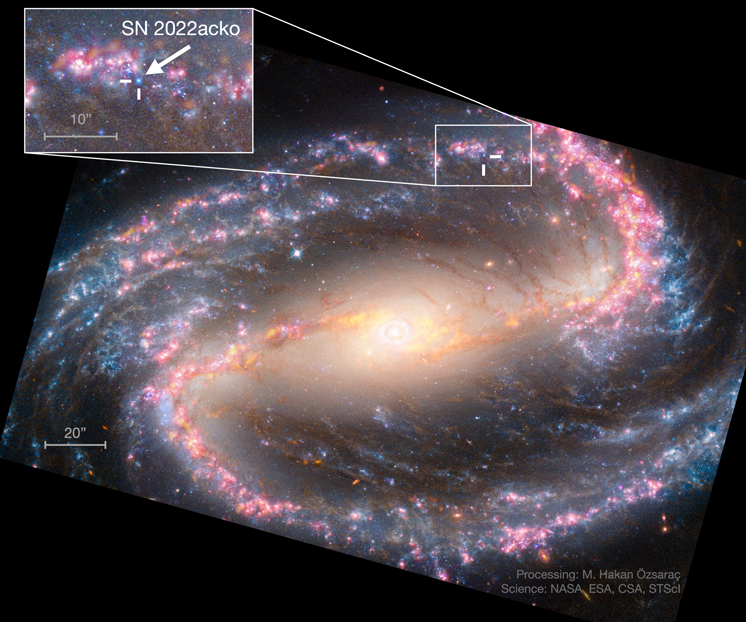
Figure 3. JWST (blue), HST (blue), VLT (red and magenta), and ALMA (yellow) composite image of NGC 1300. SN 2022acko lies in a star-forming region in a spiral arm northeast of the nucleus and is marked in both the image and the inset with white ticks. Image adapted from M. Hakan Özsaraç and Alyssa Pagan, NASA, ESA, ESO-Chile, ALMA, NAOJ, NRAO; north is up, and east is right.
Download figure:
Standard image High-resolution imageTable 3. Properties of SN 2022acko
| Property | Value |
|---|---|
| R.A. | 03h19m38 |
| Decl. |

|
| Explosion epoch | JD 2459918.67 ± 0.4 |
| Distance | 19.0 ± 2.9 Mpc |
| E(B − V)MW | 0.024 ± 0.001 mag |
| E(B − V)host | 0.03 ± 0.01 mag |
| E(B − V)total | 0.05 ± 0.01 mag |
| Host | NGC 1300 |
| Redshift | 0.00526 |
Download table as: ASCIITypeset image
We adopt a distance of 19.0 ± 2.9 Mpc from the PHANGS survey (Anand et al. 2021) derived using the numerical action method (Shaya et al. 2017; Kourkchi et al. 2020).
From our Swift observations, we confirmed that there is qualitatively little host extinction. To quantify the amount of extinction, we obtained medium-resolution spectra with Binospec (Fabricant et al. 2019) on MMT and RSS (Rangwala et al. 2008) on SALT. In these spectra the Na I D1 and D2 lines are cleanly separated for both the Milky Way and the host galaxy. We simultaneously fit the continuum and Gaussian absorption lines to the four Na I D extinction features using the astropy modeling package (Collaboration et al. 2013, 2018, 2022). We calculate the equivalent width using the continuum from this model and the spectrum itself. Using the relationship of Poznanski et al. (2012) and scaling by 0.86 to match the extinction measurements of Schlafly & Finkbeiner (2011), we measure an average E(B − V) = 0.021 ± 0.01 mag for the Na i D1 and D2 lines of the Milky Way, confirming the Schlafly & Finkbeiner (2011) value of E(B − V) = 0.026 ± 0.001 mag that we obtain from the IPAC Dust Service 33 using the supernova coordinates. With this agreement, we adopt E(B − V)MW = 0.026 ± 0.001 mag for the remainder of this Letter. For the host galaxy we measure E(B − V)host = 0.03 ± 0.01 mag from the stronger Na i D2 line, which we will use throughout this Letter.
Given that there is less than 1 day between the last nondetection and first detection, over which time SN 2022acko rose by >3.3 mag to near peak magnitude, we define the explosion epoch as the last nondetection. We take half the distance between the last nondetection and first detection as the error on the explosion epoch: 0.4 days.
4.1. Light Curve
Given the unique nature of the FUV and NUV spectra of SN 2022acko, we briefly examine its photometric properties and compare it to other well-studied supernovae to provide some context for the UV analysis. SN 2022acko rose to V-band peak brightness ∼5 days after explosion and reaching a peak brightness of V = −15.4 mag. Figure 4 shows the light curve of SN 2022acko with the left panel highlighting the last nondetection and early rise while the full light curve is shown on the right.
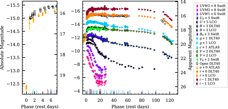
Figure 4. The absolute and extinction-corrected apparent magnitude optical and UV light curves of SN 2022acko. The left panel shows the first 7 days of evolution, highlighting the tightly constraining nondetections within 24 hr of discovery and high-cadence follow-up observations obtained immediately by the DLT40 and ATLAS surveys. No offset is applied to these filters in either panel. The DLT40 open filter is calibrated to the r band while the ATLAS o filter is similar to the r+i band (5600–8200 Å). The right panel shows the full multiband light curve, including the UV evolution. Ticks at the bottom of each panel mark epochs of spectroscopic observations with optical spectra marked in light blue and HST UV spectra shown in pink. The photometry shown this figure is available as the data behind the figure.(The data used to create this figure are available.)
Download figure:
Standard image High-resolution imageThe light-curve evolution is similar to low-luminosity supernovae (LLSNe). Using the definitions of Valenti et al. (2016) and Anderson et al. (2014), we measure the plateau slope at 50 days (s50,V = 0.35 mag(50 day−1)) and plateau length (tpt ∼ 115 days). Figure 5 shows the peak absolute magnitude and plateau slope of SN 2022acko compared to a sample of Type II supernovae from Valenti et al. (2016) and our custom database, SNDAVIS. 34 Highlighted are other supernovae of interest: LLSNe: SN 2005cs (Pastorello et al. 2006; Brown et al. 2007; Pastorello et al. 2009), SN 2012A (Tomasella et al. 2013), SN 2018lab (Pearson et al. 2023), SN 2021gmj (N. Meza-Retamal et al. 2023, in preparation); a normal Type II supernova with early-NUV spectroscopy: SN 2021yja (Vasylyev et al. 2022); and the only normal Type IIP supernova with FUV spectra: SN 1999em (Baron et al. 2000). Although the peak magnitude is similar to the LLSNe, the plateau slope is slightly steeper and plateau length slightly shorter. The evolution of SN 2022acko most closely resembles that of SN 2012A in the UV and blue optical and SN 2018lab in the red optical.
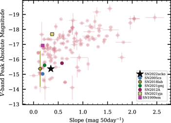
Figure 5. The V-band slope at 50 days vs. V-band peak absolute magnitude for a sample of Type II supernovae (SNDAVIS database and Valenti et al. 2016), showing that SN 2022acko (black star) is a low-luminosity supernova, similar to SN 2005cs (blue circle), SN 2018lab (mustard circle; Pearson et al. 2023), SN 2021gmj (green circle; N. Meza 2023, in preparation), and SN 2012A (magenta circle). The slope at 50 days lies between that of SN 2005cs, SN 2018lab, SN 2021gmj, and SN 2012A. We include other supernovae with important UV data sets: SN 1999em and SN 2021yja.
Download figure:
Standard image High-resolution imageThe first uvw2 observation occurs at the peak of the light curve in that filter and the uvm2 and uvw1 light curves reach peak brightness at the second data point. It is unusual to catch the UV rise, highlighting how early these observations were obtained (Pritchard et al. 2014). The UV steadily declines as both the ejecta cool and metal-line blanketing in the UV develops until SN 2022acko is no longer detected above the brightness of the underlying galaxy light (JD 2,459,933.225: uvw2, uvm2; JD 2,459,937.14: uvw1). We continued to monitor it for about 1 week beyond this, and photometry may be recovered from these observations in the future with template subtraction.
4.2. Spectroscopy
The first optical spectrum was obtained within 24 hr of discovery and spectroscopic follow-up observations continued at high cadence through the end of the HST observations, with approximately weekly spectra obtained afterwards. Figure 6 shows the close resemblance of optical spectra of SN 2022acko to those of SN 2005cs (Pastorello et al. 2006) and SN 2012A (Tomasella et al. 2013), two photometrically similar supernovae. Consistent with the photometric properties, SN 2012A has slightly broader features, while SN 2005cs has slightly narrower features. With the exception of Figure 2, the spectra in all figures have been corrected for reddening using the extinction law of Cardelli et al. (1989) and the extinction values given in Table 8.
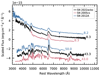
Figure 6. The optical evolution of SN 2022acko (black) is very similar to the LLSNe SN 2005cs (pink; Pastorello et al. 2006, 2009) and transitional luminosity SN 2012A (blue; Tomasella et al. 2013). The similarity of the spectra can be seen here at both ∼ 8 and ∼50 days postexplosion, with SN 2022acko falling between SN 2005cs and SN 2012A in terms of line widths (ejecta velocity).
Download figure:
Standard image High-resolution imageWe note two interesting features in the optical spectra of SN 2022acko. First, like many Type IIP supernovae observed at early times, SN 2022acko shows a ledge-like feature in the earliest spectra at 4600 Å (see Pearson et al. 2023, and references therein). Also of note is the brief presence of an absorption feature blueward of He i around day 5, which was attributed to both high-velocity He i (Pastorello et al. 2009) and N ii (Baron et al. 2000; Dessart & Hillier 2005).
5. UV Spectra
The UV spectra display a wealth of features that provide key information on the temperature, density, and chemical abundances of the outer ejecta. This can be seen in the first three UV spectra of SN 2022acko, shown in Figure 7. However, this information quickly fades as a forest of metal lines blanket the spectra, bringing all FUV flux to nearly zero within the first 20 days. This UV flux deficit is aggravated by the cooling of the photospheric layers, which causes a strong shift of the spectral energy distribution (SED) to longer wavelength until the conditions stabilize at the onset of the hydrogen recombination phase.
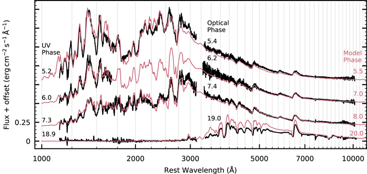
Figure 7. A time series of the extinction-corrected UV and optical spectra of SN 2022acko (black) and the well-matched CMFGEN models (pink; scaled as described in Section 5.1). The phase (in days) of each spectrum is given on the left for the UV observations, in the center for the optical observations, and on the right for the models. The day 19 spectra (observed and scaled model) are at their true flux, while the day 7 spectra are shifted by 2 × 10⁻¹⁵ erg cm−2 s−1 Å−1, the day 6 spectra are shifted by 5 × 10⁻¹⁵ erg cm−2 s−1 Å−1, and the day 5 spectra are shifted by 8 × 10⁻¹⁵ erg cm−2 s−1 Å−1. The model spectra shown in this figure are available as the data behind the figure.(The data used to create this figure are available.)
Download figure:
Standard image High-resolution imageDespite the information contained in the FUV and NUV, very little early data exist on Type II supernova. Two unusual Type II supernovae were studied early with IUE: SN 1980 K and SN 1987A (Cassatella & Fransson et al. 1987; Wu et al. 1992). SN 1980 K showed signs of interaction (Pun et al. 1995) while SN 1987A resulted from a blue supergiant (BSG) progenitor rather than a red supergiant (RSG), leading to a different evolution than expected for normal Type IIP supernovae (Walborn et al. 1987; Pun et al. 1995).
The UV spectra of SN 2022acko show strong Doppler-broadened features in the FUV and NUV that are most prominent in the first spectrum. This is the first time most of these features have been observed in the FUV of a Type IIP/L supernova. The overall flux of the UV spectra fade considerably over the first three HST epochs (3 days), most notably between 1100–1800 Å and 2050–2750 Å. The final two epochs of UV spectra contain almost zero flux, due to the severe line blanketing, except for a strong feature at 2970 Å. This highlights the need for UV observations to be obtained within 3 weeks of explosion, with earlier observations containing significantly more information. The spectral evolution can be seen in Figure 7.
Both the interstellar medium (ISM) and CSM can manifest as narrow features in the supernova spectrum (Panagia et al. 1980; Fransson et al. 1984; Schlegel & Kirshner 1998; Leonard et al. 2000; Yaron et al. 2017). UV emission lines can be interpreted as a signature of CSM interaction in Type II supernovae, especially when they have a Lorentzian profile with a narrow core and broad wings, indicating optically thick CSM. However, narrow absorption features can be associated with either optically thin CSM or ISM and are thus more challenging to associate with a supernova unless they are seen to evolve with time. The UV spectra of SN 2022acko contain a number of narrow absorption features, which we list in Table 4. Features that are present at both the host and Milky Way redshifts we associate with the ISM. With these spectra we confirm the host redshift (see Table 3). We also note that the galactic and host features are similar in depth, implying that the supernova environment is at approximately solar metallicity, perhaps slightly higher. Some features are only detected at the host redshift, although we note that these detections are at a lower S/N than the features detected in both galaxies. These features have a similarly narrow width to the features identified in both galaxies and for this reason we cannot differentiate between unshocked CSM (from the evolution of the progenitor) and an unusual ISM in the host galaxy. The lack of symmetric emission lines combined with the presence of broad absorption and P Cygni profiles indicates that at day 5 there is no optically thick CSM.
Table 4. Narrow Absorption Features Identified in the UV Spectra
| Ion | Wavelength (Å) | Source | Reference |
|---|---|---|---|
| Si iii | 1206 | galactic, host | Werk et al. (2013) |
| Fe ii/Si ii | 1260 | host | Fransson et al. (1984); Morton (2003) |
| C i/Si ii | 1280 | host | Fransson et al. (1984) |
| O i | 1302, 1304 | host | Fransson et al. (1984) |
| C ii | 1335, 1336 | galactic, host | Fransson et al. (1984) |
| N ii | 1344 | galactic, host | Fransson et al. (1984) |
| Si iv | 1394, 1403 | galactic, host | Fransson et al. (1984) |
| Si ii | 1527 | galactic, host | Fransson et al. (1984) |
| C iv | 1548, 1551 | galactic, host | Fransson et al. (1984) |
| C i | 1560, 1561 | host | Fransson et al. (1984) |
| Fe ii | 1589 | host | Morton (2003) |
| Fe ii | 1608 | galactic, host | Morton (2003) |
| He ii | 1640 | host | Fransson et al. (1984) |
| Fe ii | 2344 | galactic, host | Morton (2003) |
| Fe ii | 2383 | galactic, host | Morton (2003) |
| Fe ii | 2600 | galactic, host | Cardelli & Savage (1995) |
| Mg ii | 2796, 2802 | galactic, host | Panagia et al. (1980) |
Download table as: ASCIITypeset image
5.1. Radiative-transfer Modeling
Unlike the optical, early UV spectra are heavily affected by metal lines, producing a complex spectrum that strongly deviates from a blackbody. To identify the elements present and characterize the ejecta properties such as density and temperature we model the full UV+optical spectral evolution with the non–local thermodynamic equilibrium (NLTE) radiative-transfer code CMFGEN (Hillier & Miller 1998; Hillier & Dessart 2012; Dessart et al. 2013; Hillier & Dessart 2019).
We start with a zero-age main-sequence 12 M⊙ star at solar metallicity (Z = 0.014), evolved in Modules for Experiments in Stellar Astrophysics (MESA; Paxton et al. 2013, 2015, 2018) with default parameters and a Dutch wind scaling factor of 0.8. We chose a relatively low-mass progenitor as these are associated with underluminous events (e.g., SN 2008bk; Maund et al. 2014); however, we do not place too much emphasis on the progenitor mass as the effects of progenitor mass are degenerate with a number of other uncertain physical processes in stellar evolution (see the discussion later in the section). The preexplosion progenitor has a final mass of 9.7 M⊙, an effective temperature of 4002 K, a luminosity of 57,802 L⊙, and a radius of 500 R⊙. Its envelope composition is M(H) = 4.44 M⊙, M(He) = 3.15 M⊙, and M(O) = 0.27 M⊙. MESA artificially cuts the density profile at a Rosseland mean optical depth of 2/3 producing a dense surface (ρ ∼ 1 × 10⁻⁹ g cm−3), which is unsuitable for modeling the shock breakout phase. While material beyond this point is not important during stellar evolution, the supernova shock ionizes it, causing it to become optically thick. We extrapolate a steep density gradient beyond the surface of the original MESA model down to a density of ρ < 1 × 10⁻¹² g cm−3, including a total of 0.02 M⊙ of additional material.
A thermal bomb is used to explode the model using the radiation hydrodynamics code V1D (Livne 1993; Dessart et al. 2010a, 2010b) depositing 7.4 × 1050 erg for 0.1s between mass shells 1.55 and 1.60 M⊙ in the progenitor, producing an ejecta kinetic energy 6 × 1050 erg and an ejecta mass of 8.16 M⊙. The mass cut at 1.55 M⊙ corresponds to the neutron star gravitational mass. At day 5, the ejecta are mapped to CMFGEN, which performs the time-dependent radiation transport in NLTE assuming homologous expansion. Model ages are derived from the homologous expansion in the outer ejecta layers, neglecting the stellar radius, but assuming constant velocity since t = 0, with t = R/V (where R/V is set using a mass shell at 7800 km s−1). This supernova age is thus in tension with the explosion data, compounding with the uncertainty associated with the ∼1 day it takes the shock to reach the surface of the RSG progenitor. Comparing our homology evolution with the evolution of the model using the radiation hydrodynamics code V1D, we find agreement to within 5% for both the photospheric radius and velocity through day 20. This confirms that our assumption of homology at 5 days in CMFGEN is good and could be used to model a variety of different progenitor parameters such as metallicity, initial mass, and explosion energy. As this model was created specifically to characterize the early data presented in this Letter, we ignore a number of effects that are only important at later times when the photosphere begins to recede deep into the hydrogen-rich ejecta layers. First, we truncate the model at a minimum velocity of 2000 km s−1, excluding the deep and very optically thick inner ejecta. We also do not include 56Ni and do not treat the nonthermal effects that arise from radioactive decay.
Ideally, a model with optimized parameters would reproduce the observed flux from the UV through the IR. For this analysis we did not attempt to optimize parameters, instead using an existing model with an explosion energy of Ekin = 6 × 1050 erg. With this model, we find that, without the scaling described and shown below, the model overestimates the UV flux by a factor of 2. If this were attributed to an error in distance, NGC 1300 would have to be at 26.8 Mpc, close to 3σ above our distance estimate. The overall flux level of a supernova is affected by the explosion energy, progenitor radius, and contribution from CSM. While a full exploration of this parameter space is beyond the scope of this Letter, we explored a model with lower explosion energy (∼4 × 1050 erg). However, we found that while the overall flux of the lower-energy model was a better match to the observed flux, the line widths were too narrow and the optical flux, even at earlier times, was brighter than the observed flux when the model spectra were scaled to match the UV flux with the same method as the higher-energy model. We therefore suggest that future modeling explore different progenitor radii and CSM configurations. We note that due to degeneracies in the modeling parameters, a smaller radius could be achieved with either a lower-mass progenitor or a progenitor of the same mass but with more vigorous convection in the hydrogen envelope.
Given the mismatch between the model flux and observed flux, we scale our model flux in the following way. We redshift and redden the model using the redshift and extinction of SN 2022acko. We then scale the first model to the Swift UV photometry (uvw2, uvm2, and uvw1) at 5.5 days using a constant offset. Next, we return the model to rest wavelengths and unextinguished flux. We repeat this process on all other model spectra, applying the scaling factor derived from the first spectrum to preserve the flux evolution of the models. The observed spectra are then compared to the model at a similar phase. Figure 7 shows the results of our modeling. It is striking how well the features and flux evolution are reproduced, implying that this model is a good representation of the outer ejecta velocity, temperature, and density. Additionally, the similarity of the model and observed spectra imply that the supernova is approximately solar metallicity (see Dessart et al. 2013 for a description of the effects of metallicity on UV spectra). Given that the scaling is set by the first UV spectrum, the model reproduces the flux evolution very well in the UV, including the final epoch at day 18.9. In the optical, it slightly underestimates the flux in the early observations. It is possible that this could be solved at early times with the introduction of clumping into the model that would more rapidly shift the flux from the UV to the optical (Dessart et al. 2018), or by changing the progenitor radius, which can alter both the absolute and relative flux distribution (Dessart et al. 2013). With more optimization, a fully consistent model could be found.
Alternately, it is possible that the host extinction is underestimated. We find an additional extinction of E(B − V) = 0.03 mag produces a better fit to the first three epochs. However, the final optical spectrum at day 18.9 is overestimated by the model, which is made worse when the additional extinction is added. This could be mitigated by invoking some dust very close to the progenitor that is destroyed between days 7 and 19 by the interaction with the supernova ejecta (Fraser et al. 2012; Kochanek et al. 2012; Van Dyk et al. 2012). However, even with no extinction correction, the model is too bright at later phases, indicating that time-dependent extinction cannot fully account for the discrepancy. Although HST preexplosion observations exist (Van Dyk et al. 2023), the photometry does not constrain this mild level of extinction.
Nevertheless, the similarity of the model spectra to the observed spectra at both optical and UV wavelengths on days 5–7 indicates that there is either weak or no interaction at this phase and that the dominant radiation source is the fast moving ejecta.
As a consistency check, we performed synthetic photometry on the scaled CMFGEN model spectra to generate a synthetic light curve that we compared to the observed light curve through day 25. The trends as a function of wavelength seen in the spectroscopic comparison in Figure 7 are also apparent in the light-curve evolution. Although the scaling is set to match the first model epoch to the observed light curve in the Swift uvw2, uvm2, and uvw1 filters on day 5, the full UV evolution is very well matched by the models, including the point at which the supernova drops below detection. The optical light curve rises more slowly than the observed light curve, reaching V-band peak about 5 days after the observed light curve. Given that the model light curve does not start until day 5, when the observed light curve has flattened from its initial rise, the discrepancy between the observed and model flux is never too great. The g-, V-, r-, and i-band peaks are brighter than the observed peaks by 0.1–0.3 mag. As with the spectra, these discrepancies may be resolved by running a more customized model that varies either the progenitor radius or CSM around the progenitor.
In Figure 8 we show the spectroscopic contributions of the most prominent elements in the UV. Individual ion spectra are calculated using CMFGEN, omitting their bound–bound transitions from the formal solution to the radiative-transfer equation. The ion spectrum is then found by taking the ratio of the full spectrum to that with the ion omitted. The spectrum is most strongly influenced by Fe iii at these epochs, which produces a complex structure of absorption lines, fundamentally altering the continuum. Beyond Fe iii, we identify significant contributions from Fe ii, C iii, C ii, Ti iii, Si iv, Si iii, Si ii, S iii, S ii, Ni iii, Cr iii, Al iii, Al ii, and Mg ii. The strongest contributions from C and Si are in the FUV only and are clearly identified in our spectra. We label the relatively isolated lines in the top panel of Figure 8. As has been noted by other authors, the UV spectrum is not a continuum with emission or absorption lines but rather a continuous set of features that are blended together making it challenging to identify individual components (e.g., Pun et al. 1995; Dessart et al. 2008; Gezari et al. 2008; Dessart & Hillier 2010). With these models, we also find that the 2970 Å feature in the day 19 and 20 spectra is not emission but rather a window of lower absorption from the nearby Fe ii, Cr ii, and Ti ii absorption complexes.
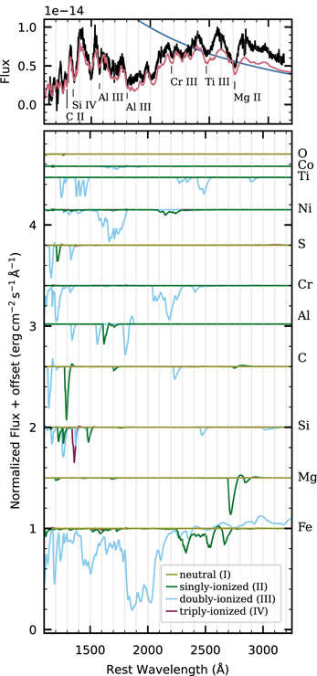
Figure 8. The identification of species present in the day 5 HST/STIS UV spectrum of SN 2022acko. Top: the UV spectrum of SN 2022acko (black) with the total CMFGEN low-energy model overplotted in pink. The CMFGEN continuum flux is shown in blue, demonstrating the strong deviation of the observed spectrum from a blackbody. Although this is a complicated region, a few fairly isolated lines are identified below the spectrum. Bottom: the contribution of the most prominent ions, grouped by species, to the full spectrum. The model spectra of individual ions in this figure are available as the data behind the figure.(The data used to create this figure are available.)
Download figure:
Standard image High-resolution imageThe ejecta radius, temperature, and velocity influence the spectroscopic properties of a supernova. Although conditions vary throughout the ejecta, we measure these quantities at the photosphere, allowing us to compare the ejecta of different supernovae. We extract these parameters for SN 2022acko from the CMFGEN model at the photosphere and compare them with other publicly available models (SN 2005cs and SN 2006bp: Dessart et al. 2008; SN 1999em: Dessart & Hillier 2006). Unlike the model for SN 2022acko, the models of SN 1999em, SN 2005cs, and SN 2006bp were computed using a steady-state version of CMFGEN that fit the observed spectra by varying the supernova luminosity, radius, and velocity. While velocity and temperature are well constrained by the ions present in the spectra and the widths of the spectral features, there is a degeneracy between the luminosity and radius that makes these values unreliable in these older models. For this reason, we do not use the original photospheric radius of the model. Instead, we derive an accurate photospheric radius using Rphot = DEPM × θEPM, where θEPM is the angular size of the photosphere and DEPM is the distance to the supernova, both derived as part of the expanding photosphere method, and a set of multiepoch steady-state CMFGEN calculations (with the method described in Dessart & Hillier 2005). The results are shown in Figure 9. The photospheric temperature, radius, and velocity all fall within the range of other Type II supernovae. The photospheric temperature is very similar to SN 2005cs: starting at ∼12,700 K on day 5.5 and decreasing to ∼6000 K by day 23.5, indicating the onset of hydrogen recombination. This implies that SN 1999em and SN 2006bp are emitting more UV flux relative to the optical flux, although the different temperatures will also affect the strength of the line blanketing. The photospheric velocity is slightly lower than SN 1999em and SN 2006bp, but significantly higher than SN 2005cs at early times, converging to a similar velocity around day 20. The velocity decreases from ∼9500 km s−1 on day 5.5 to ∼6000 km s−1 on day 23. Similarly, the photospheric radius for SN 2022acko falls between that of SN 2006bp and SN 2005cs at early times, starting with a radius of 4.5 × 1014 cm (∼6500 R⊙). It remains between these supernovae for its full evolution, although it does approach the photospheric radius of SN 1999em by day 23.5 with Rphot = 12.4 × 1014 cm (∼18,000 R⊙). These values are tabulated in Table 7 in Appendix A.
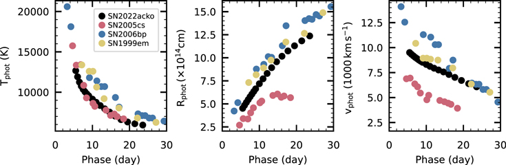
Figure 9. The photospheric evolution of SN 2022acko compared to those of SN 1999em (Dessart & Hillier 2006), SN 2005cs, and SN 2006bp (Dessart et al. 2008). The photospheric temperature (left), radius (middle), and velocity (right) fall between the derived parameters for SN 1999em, SN 2005cs, and SN 2006bp, indicating that this is not an unusual event.
Download figure:
Standard image High-resolution imageThe light-curve and spectroscopic properties of a supernova depend sensitively on the physics of stellar evolution and supernova explosions. Processes like convection (whether at the surface or the core) are not directly observable, are too complicated to model from first principles, and are computationally intensive to simulate with full physics in 3D (Goldberg et al. 2022). We are therefore still at the stage of constraining fundamental parameters, such as progenitor radius, by creating models that capture a supernova’s evolution from explosion through nebular phase at all wavelengths. One of the most comprehensive explorations of the effects of different stellar evolution and supernova explosion parameters was performed by Dessart et al. (2013). Using MESA, V1D, and CMFGEN they systematically varied one parameter at a time to explore the effects of progenitor radius (via the mixing length parameter), core overshooting, rotation, metallicity, mass loss, and explosion energy. They find that the progenitor radius can affect the light-curve rise time, luminosity, and color evolution. Progenitor metallicity, which is unaltered in the outer layers of the ejecta by explosive nucleosynthesis, affects nuclear reactions, progenitor radius, and mass loss, affecting both the light-curve shape and brightness, as well as spectroscopic features, most strongly in the UV. Unfortunately, rotation and core overshooting mimic increasing progenitor mass, creating larger He core masses, higher luminosities, higher mass-loss rates, and larger radii. While these effects are measurable, this degeneracy makes it difficult to constrain any of these parameters (Dessart & Hillier 2019). Increasing explosion energy creates a brighter and shorter plateau, increases spectral line widths, and creates more 56Ni, which creates a brighter radioactive tail phase. Although we note that there is some degeneracy here as increasing 56Ni mass increases the plateau length (Goldberg et al. 2019; Kasen & Woosley 2009). In a separate study, Dessart & Hillier (2022) find that depending on density, CSM can have a range of effects: narrow emission lines, high velocity absorption features, increased UV flux, and shallow P Cygni profiles for lower-density CSM. The success of our model in the UV indicates that the modeling of gas properties and the atomic data are satisfactory and the replication of the majority of spectroscopic features, especially the shape of the UV flux, indicates that the metallicity we selected is a good match for our observations. Given that these are the first FUV observations at this phase and the wealth of features present, this was in no way guaranteed and is a validation of the assumptions in the models. This work also validates the assumption of homology as early as 5 days after explosion, earlier than this assumption has been tested (previous work started 10–15 days after explosion), opening the door to further models at earlier times, when CSM interaction is most likely and the RSG mass loss that produces it least understood. However, the discrepant luminosity indicates that the explosion energy, radius, or CSM (or some combination) is not quite right in the model. We attempted to reduce the explosion energy but this resulted in too narrow line profiles compared to observations. Given the color dependence of this trend and the fact that CSM would increase the UV luminosity, requiring a lower explosion energy, we conclude that the most likely resolution would be a decrease in progenitor radius, although this is not a possibility that we have yet explored. A proper grid of early-time models for different progenitor masses, explosion energy, and metallicity is needed.
5.2. Comparison to Other Early UV Spectra
The number of Type IIP/L supernovae observed in the UV is very limited making it challenging to compare spectra of different supernovae at the same epoch. However, combining observations from different supernovae, it is possible to create a time series showing the UV evolution (see Figure 11).
The only FUV observation of a normal Type II supernova is SN 1999em (Baron et al. 2000), which was observed ∼12 days postexplosion and shows a significant, potentially abnormally large, flux deficit in the FUV. Two other supernovae that were well studied in the NUV by Swift are SN 2021yja (Vasylyev et al. 2022) and SN 2005cs (Brown et al. 2007). The earliest data for both of these supernovae were taken at 4 and 5 days postexplosion, respectively, and have relatively low S/N. Both of these supernovae continued to be monitored by Swift. A similar data set was collected in the NUV by GALEX for SN 2005ay, with observations starting 9 days after explosion (Gal-Yam et al. 2008). SN 2021yja was observed with HST 10 days after explosion, showing similar lines as the NUV spectra of SN 2022acko (Vasylyev et al. 2022). Additional HST NUV spectra of SN 2021yja were obtained on days 14 and 21, showing the suppression of the UV flux with time. A similar NUV spectroscopic sequence was obtained for SN 2022wsp (Vasylyev et al. 2023) with HST spectra observed on days 10 and 20. Early HST data of SN 2020fqv were also obtained, although due to high extinction, there is very little flux in the NUV observations and no flux in the FUV observation (Tinyanont et al. 2022).
We select the best spectra from this set of Type IIP/L supernovae to create the time series shown in Figure 11 using our spectra of SN 2022acko, supplemented with SN 2022wsp, SN 2021yja, SN 2005cs, and SN 1999em. For each supernova we correct for redshift and extinction and then scale the overall flux level to be approximately that of SN 2022acko at a similar phase using the values in Table 8. For supernovae that were not observed at a comparable phase, we used the already scaled spectra of SN 2021yja. While the strong Mg II (λ2800 Å) feature is visible in many spectra, all observations before day 9 lack high-enough S/N to distinguish other spectral features, with the exception of SN 2022acko. Additionally, from the strong features visible in SN 2022acko, it is clear that the day 12 FUV spectrum of SN 1999em already suffers from significant iron line blanketing and the shape of the NUV spectrum is strikingly different from the other supernovae observed at similar epochs. We note that the explosion epoch of SN 1999em is uncertain with 9 days between the last nondetection and first detection. The oldest the FUV spectrum of SN 1999em could be is 16 days, shifting it down one spectrum in Figure 11. We tested shifting and scaling the spectrum of SN 1999em to match SN 2021yja at day 14, SN 2022acko at day 19, and SN 2022wsp at day 20. We find that while the UV and optical can individually be well matched to SN 2021yja at day 14, the UV flux is smaller compared to the optical for SN 1999em. With further scaling, we find that the UV flux of SN 1999em is too high relative to the later time spectra. Both of these results are consistent with an age of 16 days; however, no UV spectrum exists at this phase with which to compare. Interestingly, this age is consistent with the age derived by Dessart & Hillier (2006) using the expanding photosphere method (EPM) method with the filter and phase combination that produces an EPM distance to the host galaxy of SN 1999em (NGC 1637) that matches the Cepheid distance (Leonard et al. 2003). The compilation of these UV spectra does not show the uniformity suggested by Gal-Yam et al. (2008). In addition to the differences noted above for SN 1999em, SN 2021yja, and SN 2022wsp continue to show NUV flux out to 20 days, possibly due to weak interaction (Dessart & Hillier 2022; Hosseinzadeh et al. 2022; Kozyreva et al. 2022; Vasylyev et al. 2023).
5.3. Missing UV Flux Fraction
While Type II supernovae peak in the UV at early times, the majority of our observations are in the optical. To calculate a bolometric luminosity, the UV contribution must be inferred from optical observations. However, as our observations show (see also Dessart & Hillier 2005; Vogl et al. 2019), a blackbody spectrum is a poor approximation of the UV flux, even as early as 5 days after explosion (Dessart et al. 2010a showed that the UV spectrum approaches a blackbody spectrum at photospheric temperatures of 30,000 K, well above the temperature of our earliest spectrum). Even when Swift observations are available, the uvw2 filter cuts off at 1600 Å. We calculate the fraction of flux redward of a given wavelength by combining our observed UV and optical spectra (linearly interpolating across the gap around 3000 Å), integrating the flux redward of a given wavelength, and comparing that to the integrated flux over the full wavelength range. The day 5 and day 7 UV spectra have been scaled (with a small uniform offset) to the UV photometry, while the final day 19 spectrum has not been scaled as the supernova is not detected in the Swift UV at this epoch. The optical spectra are scaled to the gri photometry with a linear scaling. As our spectra only span 1150–10150 Å, this analysis ignores contributions at longer and shorter wavelengths. Figure 10 shows the fraction of flux as a function of shortest wavelength observed from 1100 to 7000 Å for each epoch. We also mark the shortest wavelength in the uvw2, U, B, and V filters, indicating the fraction of flux lost when a given filter is the bluest observed. The fractional flux by filter is tabulated in Table 5.
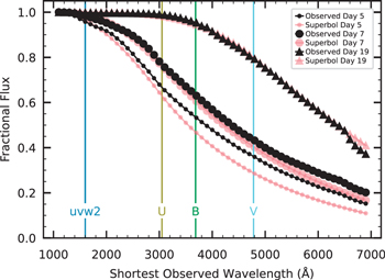
Figure 10. The observed fractional throughput (black) as a function of shortest wavelength observed for day 5 (dot), day 7 (circle), and day 19 (triangle) spectra. Plotted in pink in the fractional flux from the best-fit absorbed blackbody spectrum calculated using Equation (1) and with the same symbols representing the different epochs as were used for the observed flux. At all epochs, the absorbed blackbody approximation yields a fractional flux within 7% of the true value. The cutoff wavelengths that were used for the filters given in Table 5 are shown as vertical lines and labeled in the plot.
Download figure:
Standard image High-resolution image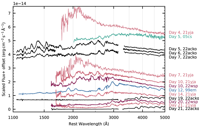
Figure 11. SN 2022acko (black) in the context of the UV evolution of Type IIP supernovae, showing the diversity of UV spectra. Swift and HST NUV spectra of SN 2021yja (pink; Vasylyev et al. 2022) span 4–21 days postexplosion. HST NUV spectra of SN 2022wsp (maroon) are shown for days 10 and 20 (Vasylyev et al. 2023). A Swift spectrum of the LLSN SN 2005cs (teal; M. Rowe 2023, in preparation) is shown as well. SN 2022acko and SN 1999em (blue; Baron et al. 2000) are the only Type IIP/L supernovae with FUV spectra, with the first epochs of SN 2022acko observed significantly earlier than SN 1999em, resulting in strong FUV features. Iron line blanketing is already significantly suppressing the FUV flux by day ∼12 in the SN 1999em spectrum.
Download figure:
Standard image High-resolution imageTable 5. Fraction of Flux Redward of a Given Wavelength
| Shortest Filter | Wavelength Range (Å) | Fraction of Flux (Day 5) | Fraction of Flux (Day 7) | Fraction of Flux (Day 19) |
|---|---|---|---|---|
| uvw2 | 1600–10150 | 0.96 | 0.98 | 1.00 |
| U | 3050–10150 | 0.67 | 0.76 | 0.99 |
| B | 3685–10150 | 0.54 | 0.63 | 0.95 |
| V | 4780–10150 | 0.36 | 0.44 | 0.79 |
Download table as: ASCIITypeset image
Over time, as the peak of the SED shifts to the optical, the majority of the flux is captured with filters accessible from ground-based observatories. We find the majority of the flux is captured when the bluest filter is the Swift uvw2 filter. However, only 53% of the flux is captured at day 5 if the bluest filter is the B band. This fraction of observed flux increases to 63% 2 days later as the SED peak shift redward and is at 95% by day 19.
We characterize the observed spectra as a blackbody that undergoes absorption as a function of wavelength, for wavelengths shortward of a cutoff wavelength as described in Nicholl et al. (2017) and implemented in the code SuperBol (Nicholl 2018a, 2018b). Briefly, we fit the equation

where A is a scale factor, Bλ is the Plank function, T is the temperature in K, and λcutoff is the cutoff wavelength in Å. We find the spectra are well approximated by this functional form with the best-fit parameters for each epoch given in Table 6. It is interesting that the temperatures derived from this method are significantly higher than those of our CMFGEN model, indicating that while this is a good empirical description of the spectra, it may not be appropriate for characterizing the physical conditions of the ejecta, especially at early times. A comparison of the observed fractional flux and fractional flux from the analytic SuperBol parameterization is shown in Figure 10. At early times, the absorbed blackbody approximation underestimates the fractional throughput with a maximum difference of ∼7%, with the effect decreasing over time and as the shortest wavelength observed moves redward.
Table 6. Absorbed Blackbody Parameters
| Phase | Temperature (K) | x | λcutoff | Scale Factor |
|---|---|---|---|---|
| 5 | 21,750 | 2.3 | 2960 | 3.5 × 10⁻³¹ |
| 7 | 14,150 | 2.0 | 2990 | 9.9 × 10⁻³¹ |
| 19 | 7425 | 2.54 | 4815 | 6.2 × 10⁻³⁰ |
Download table as: ASCIITypeset image
6. Conclusion
In this Letter we present the first early FUV spectra of a Type IIP/L supernova. SN 2022acko is similar to SN 2012A, SN 2005cs, SN 2018lab, and SN 2021gmj with a faint V-band peak magnitude of V = −15.4 mag and plateau slope of s50,V = 0.35 mag (50 day−1). Discovered within 24 hr of explosion, we obtained high-cadence photometry in the UV and optical to capture the early evolution. With these observations and the classification as a Type II supernova, we triggered our disruptive ToO program with the FUV and NUV detectors on HST/STIS.
These observations, executed 5, 6, and 7 days after explosion, show a wealth of FUV and NUV features that fade over time. Two more observations, taken 19 and 21 days after explosion, show the (expected) complete suppression of flux in the UV. In the first epoch, we identify narrow absorption features, many of which we attribute to both the Milky Way and host galaxy ISM. Some narrow features are seen only at the host galaxy redshift and can either be due to CSM or ISM. We model the supernova spectra with CMFGEN, finding good agreement with the Ekin = 6 × 1050 erg explosion of a 12 M⊙ star at solar metallicity. With this modeling we identify notable contributions from Mg, Si, C, Al, Cr, S, Ni, and Ti with the majority of the structure coming from Fe. Using the CMFGEN models, we extract the photospheric temperature, radius, and velocity of SN 2022acko and compare it to SN 1999em, SN 2005cs, and SN 2006bp. SN 2022acko falls within the range set by these supernovae for each parameter demonstrating that its photospheric properties are normal for a Type II supernova. Dessart & Hillier (2005) showed that the UV is strongly affected by metals, whose abundance is primordial at these early postexplosion epochs. While the abundances of metals, such as Fe, can be measured through the forest of lines they produce over extended spectral regions, He, C, N, O, Mg, and Al have resonance transitions in the UV that produce strong, isolated lines that would vary with metallicity and potentially CNO processing (Davies & Dessart 2019). With more detailed modeling and more spectra to compare to, it is possible that these spectra could be used to measure relative metallicity (e.g., Dessart & Hillier 2005; Foley & Kirshner2013; although see also Dessart et al. 2014; Graham et al. 2015; DerKacy et al. 2020, 2023).
We compare the spectra of SN 2022acko to the best UV data available, using spectra of SN 2005cs, SN 1999em, SN 2021yja, and SN 2022wsp. In these spectra we see hints of great diversity in the UV; however, it is challenging to draw a true comparison given the sparse time sampling, low S/N, host galaxy extinction, and rapid UV evolution. Interestingly, we do not see narrow or intermediate width emission lines or P Cygni profiles associated with CSM interaction in the UV for SN 2022acko, indicating that it is either not there, at too low density to produce emission lines, or has been swept up by the ejecta already. Even earlier observations would further constrain the characteristics of any CSM present as well as a more detailed examination of observations at other wavelengths (e.g., radio nondetection; Ryder et al. 2022).
Finally, we investigate the fraction of flux observed for a variety of scenarios, finding on day 5 that 53% of the flux is captured when the B band is the bluest filter observed, while 95% of the flux is captured when observations extend to the uvw2 filter. The percentage of missing flux decreases over time as the ejecta cools, highlighting the importance of even earlier UV observations, when the majority of the flux falls below 3000 Å. We fit an absorbed blackbody to our full spectra, finding that the functional form of Nicholl et al. (2017) effectively characterize the shape of the spectrum, provided the right parameters are used, matching the observed fractional flux to within 10%.
The collection of this UV data set took the mobilization and coordination of both ground- and space-based resources with rapid response time through multiple collaborations. With these observations it is clear that collecting early UV spectra is worth the effort: there is a wealth of information in the UV that we are only beginning to characterize. Understanding the diversity of Type II supernovae in the UV will be critical for interpreting high-redshift supernovae coming from the earliest stellar populations. This can only currently be accomplished with HST. However, in the future, the rapid response of the proposed Ultraviolet Explorer (UVEX; Kulkarni et al. 2021) could extend these observations even earlier, allowing us to probe the earliest phases of evolution and possible interaction with CSM.
In addition to the unique observations presented in this Letter, a rich data set has already been collected on SN 2022acko, encompassing a number of other firsts. It was the first supernova to use JWST observations to identify the progenitor of a supernova in HST preexplosion images (Van Dyk et al. 2023; see also C. Kilpatrick et al. 2023, in preparation) and the first core-collapse supernova for which JWST spectroscopy was obtained (see M. Shahbandeh et al. 2023, in preparation). We will continue to observe SN 2022acko into the nebular phase, making it a keystone event that can be used to interpret future supernova observations.
Acknowledgments
K.A.B. thanks everyone at STScI for their work in getting this program scheduled and executed quickly, especially contact scientist TalaWanda Monroe and program coordinator Blair Porterfield. We thank our referee for their time and comments that resulted in an improved paper. K.A.B thanks M. Hakan Özsara for the use of the image of NGC 1300. This publication was made possible through the support of an LSSTC Catalyst Fellowship to K.A.B., funded through grant 62192 from the John Templeton Foundation to LSST Corporation. The opinions expressed in this publication are those of the authors and do not necessarily reflect the views of LSSTC or the John Templeton Foundation. Time domain research by the University of Arizona team and D.J.S. is supported by NSF grants AST-1821987, 1813466, 1908972, and 2108032, and by the Heising-Simons Foundation under grant #20201864. The research by Y.D., S.V., N.M., and E.H. is supported by NSF grant AST-2008108. J.I.G.H. acknowledges financial support from the Spanish Ministry of Science and Innovation (MICINN) project PID2020-117493GB-I00. D.J.H. thanks NASA for partial support through the astrophysical theory grant 80NSSC20K0524. L.G. and T.E.M.B. acknowledge financial support from the Spanish Ministerio de Ciencia e Innovación (MCIN), the Agencia Estatal de Investigación (AEI) 10.13039/501100011033, the European Social Fund (ESF) “Investing in your future,” and the European Union Next Generation EU/PRTR funds under the PID2020-115253GA-I00 HOSTFLOWS project, the 2019 Ramón y Cajal program RYC2019-027683-I, the 2021 Juan de la Cierva program FJC2021-047124-I, and from Centro Superior de Investigaciones Científicas (CSIC) under the PIE project 20215AT016, and the program Unidad de Excelencia María de Maeztu CEX2020-001058-M. C.A. and J.D. acknowledge support by NASA grants JWST-GO-02114.032-A and JWST-GO-02122.032-A. This work is supported by the international Gemini Observatory, a program of NSF’s NOIRLab, which is managed by the Association of Universities for Research in Astronomy (AURA) under a cooperative agreement with the National Science Foundation, on behalf of the Gemini partnership of Argentina, Brazil, Canada, Chile, the Republic of Korea, and the United States of America. E.B. was supported in part by NASA grant 80NSSC20K0538. The SALT data presented in this paper were obtained via Rutgers University program 2022-1-MLT-004 (PI: S.W.J.). L.A.K. acknowledges support by NASA FINESST fellowship 80NSSC22K1599. This Letter used data obtained with the MODS spectrographs built with funding from NSF grant AST-9987045 and the NSF Telescope System Instrumentation Program (TSIP), with additional funds from the Ohio Board of Regents and the Ohio State University Office of Research. This research is based on observations made with the NASA/ESA Hubble Space Telescope obtained from the Space Telescope Science Institute, which is operated by the Association of Universities for Research in Astronomy, Inc., under NASA contract NAS 5-26555. These observations are associated with program 17132. Support for program 17132 was provided by NASA through a grant from the Space Telescope Science Institute, which is operated by the Association of Universities for Research in Astronomy, Inc., under NASA contract NAS 5-26555. This research was supported by the Munich Institute for Astro-, Particle and BioPhysics (MIAPbP) which is funded by the Deutsche Forschungsgemeinschaft (DFG, German Research Foundation) under Germany’s Excellence Strategy—EXC-2094-390783311. The INT is operated on the island of La Palma by the Isaac Newton Group of Telescopes in the Spanish Observatorio del Roque de los Muchachos of the Instituto de Astrofísica de Canarias. This work makes use of observations from the Las Cumbres Observatory network. The LCO team is supported by NSF grants AST-1911225 and AST-1911151.
J.S. acknowledges support from the Packard Foundation.
This work was based partially on observations obtained at the Southern Astrophysical Research (SOAR) telescope, which is a joint project of the Ministério da Ciência, Tecnologia e Inovações (MCTI/LNA) do Brasil, the US National Science Foundations NOIRLab, the University of North Carolina at Chapel Hill (UNC), and Michigan State University (MSU).
This research has made use of the NASA/IPAC Extragalactic Database (NED), which is funded by the National Aeronautics and Space Administration and operated by the California Institute of Technology. This research made use of Photutils, an Astropy package for detection and photometry of astronomical sources (Bradley et al. 2022).
Facilities: ADS - , Bok (B&C) - Steward Observatory 2.3 meter Bok Telescope, CTIO:PROMPT - Panchromatic Robotic Optical Monitoring and Polarimetry Telescopes at Cerro Tololo Inter-American Observatory, HST (STIS) - Hubble Space Telescope satellite, IRSA - , LBT (MODS) - Large Binocular Telescope Observatory, LCOGT (SBIG - , Sinistro - , FLOYDS) - , MMT (Binospec) - MMT at Fred Lawrence Whipple Observatory, Meckering:PROMPT - , NED - , SALT (RSS) - Southern African Large Telescope, SOAR (GHTS) - The Southern Astrophysical Research Telescope, Swift (UVOT) - Swift Gamma-Ray Burst Mission, TNS - .
Software: Astropy (Astropy Collaboration et al. 2013, 2018, 2022), Binospec IDL (Kansky et al. 2019), BANZAI (McCully et al. 2018), CMFGEN (Hillier & Miller 1998; Hillier & Dessart 2012; Dessart et al. 2013; Hillier & Dessart 2019), FLOYDS (Valenti et al. 2014), HOTPANTS (Becker 2015), IDSRED (Bravo 2023), IRAF (Tody 1986, 1993), LCOGTSNpipe (Valenti et al. 2016), Light Curve Fitting (Hosseinzadeh et al. 2023), MatPLOTLIB (Hunter 2007), MESA (Paxton et al. 2011, 2013, 2015, 2018, 2019), MODS pipeline (Pogge 2019), NumPy (Harris et al. 2020), Photutils (Bradley et al. 2022), PySALT (Crawford et al. 2010), SuperBol (Nicholl 2018a), Scipy (Virtanen et al. 2020), V1D (Livne 1993).
Appendix A: Photospheric Parameters for SN 2022acko
Table 7 gives the temperature, radius, density, and velocity of the photosphere of the CMFGEN model of SN 2022acko as a function of time.
Table 7. Photospheric Properties of SN 2022acko
| Age (days) | Radius (1014 cm) | Velocity (km s−1) | Temperature (K) |
|---|---|---|---|
| 5.5 | 4.518 | 9508 | 12,669 |
| 6.0 | 4.839 | 9335 | 11,910 |
| 6.5 | 5.157 | 9182 | 11,247 |
| 7.0 | 5.461 | 9029 | 10,746 |
| 7.5 | 5.768 | 8901 | 10,357 |
| 8.0 | 6.056 | 8761 | 10,052 |
| 8.5 | 6.346 | 8641 | 9790 |
| 9.0 | 6.631 | 8529 | 9555 |
| 10.0 | 7.185 | 8316 | 9141 |
| 11.0 | 7.720 | 8123 | 8752 |
| 12.1 | 8.300 | 7939 | 8349 |
| 13.3 | 8.925 | 7761 | 7943 |
| 14.6 | 9.569 | 7565 | 7533 |
| 16.1 | 10.167 | 7309 | 7047 |
| 17.7 | 10.742 | 7020 | 6603 |
| 19.5 | 11.297 | 6712 | 6310 |
| 21.4 | 11.835 | 6391 | 6093 |
| 23.6 | 12.367 | 6073 | 5932 |
Download table as: ASCIITypeset image
Appendix B: Comparison Supernovae
Table 8 gives the extinction, redshift, distance modulus, and explosion epoch for each of the supernovae in the spectroscopic evolution sequence in Figure 11.
Table 8. Parameters Used for Comparison Supernovae
| Supernova | E(B − V)MW | E(B − V)host | Redshift | Distance | Explosion Epoch | Reference |
|---|---|---|---|---|---|---|
| (mag) | (mag) | Modulus | (JD) | |||
| SN 2022wsp | 0.05 | 0.3 | 0.00932 | 31.99 | 2,459,855.08 ± 0.42 | Vasylyev et al. (2023), |
| Lu et al. (1993) | ||||||
| SN 2021yja | 0.0191 | 0.085 | 0.00568 | 31.85 | 2,459,464.9 ± 0.06 | Hosseinzadeh et al. (2022) |
| SN 2012A | 0.0274 | 0.009 | 0.00251 | 29.53 | 2,455,933.5
| Tomasella et al. (2013), |
| Silverman et al. (2017), | ||||||
| Tully (1988) | ||||||
| SN 2005cs | 0.034 | 0.015 | 0.00154 | 29.39 | 2,453,549.5 ± 1 | Baron et al. (2007), |
| Sabbi et al. (2018), | ||||||
| Pastorello et al. (2006), | ||||||
| Silverman et al. (2017) | ||||||
| SN 1999em | 0.035 | 0.1 | 0.00239 | 30.34 | 2,451,475.9±2 | Elmhamdi et al. (2003), |
| Leonard et al. (2003) |
Download table as: ASCIITypeset image
Footnotes
- 29
- 30
- 31
- 32
- 33
- 34