Abstract
We present our study on the spatially resolved Hα and M* relation for 536 star-forming and 424 quiescent galaxies taken from the MaNGA survey. We show that the star formation rate surface density ( ), derived based on the Hα emissions, is strongly correlated with the M* surface density (
 ) on kiloparsec scales for star-forming galaxies and can be directly connected to the global star-forming sequence. This suggests that the global main sequence may be a consequence of a more fundamental relation on small scales. On the other hand, our result suggests that ∼20% of quiescent galaxies in our sample still have star formation activities in the outer region with lower specific star formation rate (SSFR) than typical star-forming galaxies. Meanwhile, we also find a tight correlation between
  and
and  for LI(N)ER regions, named the resolved “LI(N)ER” sequence, in quiescent galaxies, which is consistent with the scenario that LI(N)ER emissions are primarily powered by the hot, evolved stars as suggested in the literature.
1. Introduction
It has been known for more than a decade that star-forming galaxies form a tight sequence on the star formation rate and stellar mass plane, the so-called “star formation main sequence” (SFMS; Brinchmann et al. 2004; Daddi et al. 2007; Noeske et al. 2007; Pannella et al. 2009; Karim et al. 2011; Whitaker et al. 2012; Speagle et al. 2014). The origin of the main sequence is often attributed to the smooth mode of the star formation in galaxies due to continuous accretion of the gas supply (Noeske et al. 2007). However, it has been challenging to reproduce the observed normalization and slope of the main sequence in hydrodynamical simulations and semi-analytical models (Davé 2008; Damen et al. 2009).
One of the keys to understanding the origin of the tight correlation between SFR and M* is through the probe of these two quantities on smaller scales, i.e., the surface densities of SFR and M*( and
and  , respectively). If the relation between
  and
and  still holds on small scales, it would suggest that the global SFR–M* relation is primarily the outcome of the local correlation and the mechanism that drives the star formation activity with respect to the stellar mass could be universal across various physical scales, similar to the situation where the well-known Kenicutt–Schmidt relation (Kennicutt 1998a) between the star formation rate surface density and the cold gas surface density is found both locally (e.g., Bigiel et al. 2008) and globally. On the other hand, the lack of the correlation between
  and
and  would otherwise suggest a galaxy-wide process that regulates the SFR of galaxies as a whole. Rosales-Ortega et al. (2012) and Sánchez et al. (2013) first show a tight correlation between the stellar surface mass density and the surface star formation density for H ii regions in nearby galaxies selected from the Calar Alto Legacy Integral Field Area survey (CALIFA; Sánchez et al. 2012). Later on, it was found that at
  ,
,  in general traces the underlying
  (Wuyts et al. 2013; Nelson et al. 2016) using data from 3D-HST and CANDELS. Recently, Cano-Díaz et al. (2016) made a deeper analysis using the CALIFA data and quantified the slope and amplitude of the resolved
  and M* relation on kiloparsec scales for nearby galaxies and showed that similar to
  galaxies, the spatially resolved relation also holds for star-forming galaxies in the local universe.
In this Letter, we study the extinction-corrected Hα surface density ( ) as a function of
  for nearby galaxies taken from the MaNGA survey. We not only double the sample size of local star-forming galaxies compared to Cano-Díaz et al. (2016), but also extend the analysis to the quiescent population. In addition, for the first time, we show that
  and
and  form two separate sequences for the H ii and LI(N)ER regions in quiescent galaxies. Throughout this Letter we adopt the following cosmology: H0 = 100h
  Mpc−1 with h = 0.7,
  , and
, and  . We use a Salpeter initial mass function (IMF) and the conversion from Kennicutt (1998b): SFR(
 yr−1) =
  (Hα) (erg s−1) when deriving the star formation rate from Hα.
2. Data and Sample Selection
MaNGA is an IFU program to survey for 10,000 nearby galaxies with a spectral resolution varying from R ∼1400 at 4000 Å to R ∼2600 at 9000 Å (Law et al. 2015; Yan et al. 2016; Blanton et al. 2017). The targets are selected to represent the overall galaxy population with stellar masses greater than  at
at  . The angular size of each spaxel is 0
5, while the average FWHM of the MaNGA data is 2
5, and therefore ∼20 neighboring spaxels are correlated. The average number of spaxels is 800 per galaxy. Our sample was drawn from the SDSS DR13 release (Albareti et al. 2017) containing 1392 galaxies, processed with the MPL-4 version of the MaNGA data reduction pipeline (Law et al. 2015). We adopt Pipe3D pipeline (Sánchez et al. 2016a) to perform the spectral line fitting, following the fitting procedures described in Sánchez et al. (2016b). The stellar continuum was first modeled with a linear combination of 156 single stellar population templates with 39 ages and 4 stellar metallicities that were extracted from the synthetic stellar spectra from the GRANADA library (Martins et al. 2005) and the MILES project (Sánchez-Blázquez et al. 2006). Then,
 is obtained using the stellar populations derived for each spaxel. To measure the emission-line fluxes, we subtract the best-fit stellar continuum from the reduced data spectrum. The dust extinction of the emission-line fluxes is corrected by using the Balmer decrement, adopting the Calzetti extinction law (Calzetti 2001) with RV = 4.5 (Fischera & Dopita 2005).
In this analysis, we confine our sample to galaxies that are not under interactions with other objects by excluding galaxies that have a spectroscopically confirmed companion using the NSA catalog15 or those identified as mergers identified by the Galaxy Zoo project (Darg et al. 2010a, 2010b). The final sample consists of 1085 galaxies.
Since the Hα emission may be powered by various sources (e.g., star formation, AGNs, old evolved stars, etc.), we apply both the standard Baldwin–Phillips–Terlevich (Baldwin et al. 1981; Veilleux & Osterbrock 1987; Kauffmann et al. 2003; Kewley et al. 2006) excitation diagnostic diagrams and the WHAN diagram (Cid Fernandes et al. 2011) to classify the emission-line regions. More specifically, we adopt the [O iii] 5007/Hβ versus [S ii] 6717 + 6731/Hα diagnostic with the dividing curves suggested in the literature (e.g., Kewley et al. 2001; Kauffmann et al. 2003; Cid Fernandes et al. 2010) to select “H ii” and “LI(N)ER” regions, and then use more conservative criteria (i.e., log([N ii]/Hα) < −0.4 and  Å for H ii regions and
  Å for LI(N)ER regions, where W is equivalent width) than those suggested in Cid Fernandes et al. (2011) to further clean our selections.
To study the resolved star formation activity in each galaxy, we define a quantity “H ii fraction,” which is the ratio between the number of H ii spaxels and the number of spaxels within 1.5× effective radius ( ), which also meet at least one of the following criteria: S/N(continuum) > 3, S/N(Hα) > 2, S/N(Hβ) > 2, S/N([O iii]) > 2, S/N([S ii]) > 2, and S/N([N ii]) > 2. The H ii fractions of our sample are color-coded and shown in the SFR–M* relation plot (the upper panel of Figure 1). The SFR and M* measurements are directly taken from the public MPA-JHU catalog.16
Since the Kroupa IMF (Kroupa 2001) is adopted in the MPA-JHU catalog while we use the Salpeter IMF (Salpeter 1955), we add 0.2 dex to the MPA-JHU measured SFR and M* to compensate for the differences.
), which also meet at least one of the following criteria: S/N(continuum) > 3, S/N(Hα) > 2, S/N(Hβ) > 2, S/N([O iii]) > 2, S/N([S ii]) > 2, and S/N([N ii]) > 2. The H ii fractions of our sample are color-coded and shown in the SFR–M* relation plot (the upper panel of Figure 1). The SFR and M* measurements are directly taken from the public MPA-JHU catalog.16
Since the Kroupa IMF (Kroupa 2001) is adopted in the MPA-JHU catalog while we use the Salpeter IMF (Salpeter 1955), we add 0.2 dex to the MPA-JHU measured SFR and M* to compensate for the differences.
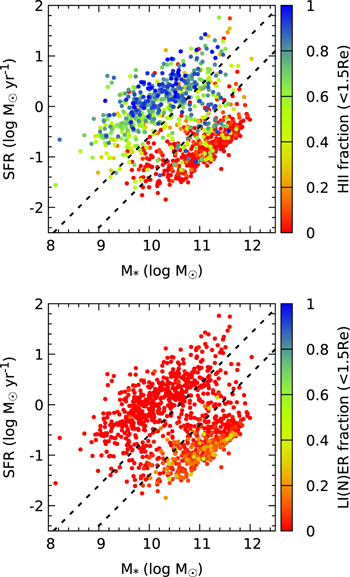
Figure 1. Global SFR–M* relation with color-coded H ii and LI(N)ER fractions. The black dashed lines in both panels indicate two constant SSFRs: −10.6 log(SFR  ) and −11.4 log(SFR
  ). See the text for details.
Download figure:
Standard image High-resolution imageThere are two loci in this plot—the top left locus is the SFMS while the bottom right locus is referred to as the quiescent population. As revealed in this figure, most galaxies in the SFMS have H ii fractions greater than 50% (in green and blue), while the quiescent sequences are dominated by galaxies with H ii fractions less than 50% (in orange and red). Similarly, we show the LI(N)ER fraction in the bottom panel of Figure 1. It can be seen that quiescent galaxies have higher LI(N)ER fractions than star-forming galaxies, but none is higher than 0.6.
To select galaxies in both sequences for detailed analysis, we apply two cuts with constant specific star formation rates (SSFRs; shown as black dashed lines in Figure 1). Galaxies with an SSFR greater than −10.6 log(SFR  ) and those with an SSFR less than −11.4 log(SFR
  ) are selected as the star-forming and quiescent populations, respectively. Galaxies between the two cuts are in the green valley and will not be discussed in this Letter. After these selections, there are 960 galaxies left for our analysis.
3. Results
3.1.
 – Relation for Star-forming Galaxies


To study the  –
– relation for galaxies at different redshifts, we need to compensate for the different physical size of spaxels. Therefore, we convert the units of both
  and
and  from per spaxel to per kpc2, with inclination correction. The inclination angle is derived using
  , where i is the inclination angle, α is the intrinsic axis ratio, and b/a is the observed ratio from the NSA catalog. We use
  for our analyses. The redshift information needed for this conversion is directly from the Pipe3D catalog.
The  –
– relation of the H ii spaxels of the star-forming galaxies is shown in Figure 2(a). The two black dashed lines indicate two constant SSFRs, −10.6 log(SFR
  ) and −11.4 log(SFR
  ), respectively, which are identical to those shown in the global SFR–M* relation plot (Figure 1), as references. We perform a linear fitting with the ordinary least squares method (OLS). The slope and zero-point (ZP) of the best fit (orange solid line) are 0.715 ± 0.001 and 33.204 ± 0.008, respectively. We also perform the “orthogonal distance regression” (ODR) fitting, which is to minimize the sum of the squares of both the x residual and the y residual, and thus is more suitable for investigating the relation between two quantities. By using the ODR fitting, the slope and zero-point of the best fit (red solid line) are 1.005 ± 0.004 and 30.922 ± 0.014, respectively. As shown in Figure 2, the ODR best fit better represents the trend of the distribution than the OLS best fit. The fitting results using OLS and ODR are also summarized in Table 1. The values of zero-point in parenthesis are SFR densities in the unit of log(
 yr−1 kpc−2).
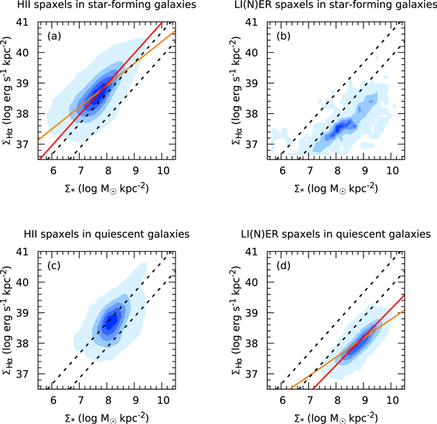
Figure 2. The  –
– relations for H ii and LI(N)ER spaxels in star-forming and quiescent galaxies. The blue color scheme of the contour indicates 1%, 20%, 40%, 60%, and 80% of the peak density. The two black dashed lines are identical to those in Figure 1. The orange and red solid lines indicate the best-fit lines using the OLS and ODR methods, respectively. See the text for details.
Download figure:
Standard image High-resolution imageTable 1. Fitting Results
| Star-forming | Quiescent | |
|---|---|---|
| (H ii regions) | (LI(N)ER regions) | |
| Slope (OLS) | 0.715 ± 0.001 | 0.620 ± 0.005 |
| ZP (OLS) | 33.204 (−8.056) ± 0.008 | 32.584 ± 0.045 |
| Scattera (OLS) | 0.159 | 0.095 |
| Slope (ODR) | 1.005 ± 0.004 | 0.922 ± 0.016 |
| ZP (ODR) | 30.922 (−10.338) ± 0.014 | 29.901 ± 0.113 |
| Scattera (ODR) | 0.127 | 0.071 |
Note.
aVariance of residuals, defined as the weighted sum of squared residuals divided by degrees of freedom.Download table as: ASCIITypeset image
We further compare our fitting results with Cano-Díaz et al. (2016), who study the spatially resolved SFR versus stellar mass relation for SFMS galaxies using data from CALIFA. Although the definitions of star-forming and quiescent galaxies are a bit different between Cano-Díaz et al. (2016) and this Letter, our OLS fitting results are consistent with Cano-Díaz et al. (2016). We also perform the ODR fitting for the data from Cano-Díaz et al. (2016) and the results are again consistent with each other. The uncertainties of the fitting results in this Letter are one order of magnitude smaller compared to Cano-Díaz et al. (2016) because of the larger sample size of the MaNGA survey.
We repeat the same analysis for LI(N)ER spaxels and the result is shown in Figure 2(b). At a given  , the
, the  for the LI(N)ER spaxels is lower than that for H ii spaxels by more than one order of magnitude. As the number of LI(N)ER spaxels is too small for statistical meaningful analysis, we do not perform line fitting for this category.
3.2.
– Relation for Quiescent Galaxies


We next investigate the relation between the Hα surface density and stellar mass surface density for the quiescent galaxies. We repeat the same procedure for the H ii/LI(N)ER spaxels as done for the SFMS, except the inclination angle correction, since it is non-trivial to estimate the inclination angles of quiescent galaxies from the observed axis ratio. The results are shown in Figures 2(c) and (d).
Interestingly, a positive correlation between  –
– is also observed for H ii spaxels but with lower SSFR by ∼0.5 dex compared to the H ii spaxels in star-forming galaxies. This offset is not totally unexpected since the quiescent population is either in the process of undergoing quenching or has already experienced quenching, which may alter the resolved
  –
– relation.
To further investigate the properties of the H ii spaxels in quiescent galaxies, we make plots to show the radial distributions of the H ii and LI(N)ER fractions for both star-forming and quiescent galaxies. The results are shown in Figure 3. We divide the sample into three categories: 536 star-forming galaxies, 92 quiescent galaxies with H ii fractions greater than 0.1, and 332 quiescent galaxies with H ii fractions less than 0.1. For a given spaxel, the radius is computed using  for a star-forming galaxy and
 ![$R\,=\sqrt{{x}^{2}+{[y/(b/a)]}^{2}}$](https://content.cld.iop.org/journals/2041-8205/851/2/L24/revision1/apjlaa9d80ieqn59.gif) for a quiescent galaxy, where i is the inclination angle and b/a is the axis ratio. For star-forming galaxies, H ii spaxels dominate from the core to outskirts, as expected. For quiescent galaxies with high H ii fractions, the H ii fractions decrease toward the center while the LI(N)ER fractions increase toward the center. For quiescent galaxies with low H ii fractions, LI(N)ER fraction is higher than the H ii fraction across the entire galaxies, except for the area beyond
for a quiescent galaxy, where i is the inclination angle and b/a is the axis ratio. For star-forming galaxies, H ii spaxels dominate from the core to outskirts, as expected. For quiescent galaxies with high H ii fractions, the H ii fractions decrease toward the center while the LI(N)ER fractions increase toward the center. For quiescent galaxies with low H ii fractions, LI(N)ER fraction is higher than the H ii fraction across the entire galaxies, except for the area beyond  . These galaxies are similar to cLIERs and eLIERs described in Belfiore et al. (2016).
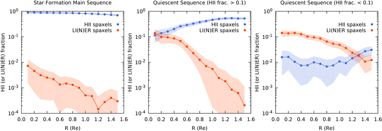
Figure 3. Radial distributions of H ii and LI(N)ER fractions. Panels from left to right are for star-forming galaxies, quiescent galaxies with H ii fractions greater than 0.1, and quiescent galaxies with H ii fractions less than 0.1. See the text for details.
Download figure:
Standard image High-resolution imageMost of the H ii spaxels in quiescent galaxies shown in Figure 2(c) belong to the quiescent galaxies with high H ii fractions (e.g., the middle panel of Figure 3). Combining the results from the two figures suggests that ∼20% of quiescent galaxies in our sample still have star formation activities in the outer region with lower resolved SSFR than typical star-forming galaxies, consistent with the results conducted by Ellison et al. (2017).
Next, we discuss the LI(N)ER spaxels. The LI(N)ER fractions are much higher than the H ii fractions in quiescent galaxies, as shown in Figure 1. Although “LI(N)ERs” are often referred to as low ionization nuclear emission-line regions (Heckman 1980), previous works have shown that the “LI(N)ER” region is not only confined in the galactic nuclei but can extend to several kiloparsecs (Belfiore et al. 2016, 2017). In addition to low activity AGNs, other possible ionizing sources of LI(N)ERs also include hot evolved stars (Binette et al. 1994; Sarzi et al. 2010; Cid Fernandes et al. 2011; Yan & Blanton 2012) and shocks (Dopita 1995; Dopita et al. 2015). Studying the spatial distributions of LI(N)ER regions as well as how the strength of emissions depends on the stellar mass may shed lights on the origin of LI(N)ER emissions.
Figure 2(d) shows that the LI(N)ER spaxels also form a very tight correlation between  and
and  . We perform both the OLS and ODR fittings for the LI(N)ER distribution. The slope and zero-point of the OLS best fit (orange solid line) are 0.620 ± 0.005 and 32.584 ± 0.045, respectively. The slope and zero-point of the ODR best fit (red solid line) are 0.922 ± 0.016 and 29.901 ± 0.113, respectively. The fitting results are summarized in Table 1.
Previously, Sarzi et al. (2010) have already shown that the Hβ flux closely traces the stellar continuum for early-type galaxies selected from the SAURON sample. The tight correlation we find between the Hα surface density and stellar mass surface density for LI(N)ER spaxels, named “resolved LI(N)ER sequence,” is thus not totally surprising. However, this is the first time we show that the Hα emissions are directly correlated with the underlying stellar mass surface density. This can be consistent with the hot, evolved stars as the dominant mechanism powering the Hα emissions in quiescent galaxies. A more detailed analysis comparing the properties of LI(N)ER regions between star-forming and quiescent galaxies will be presented in a forthcoming paper (K. Zhang et al. 2017, in preparation).
3.3. Spatially Resolved versus Global Hα (SFR)–M* Distribution
The correlation between the star formation rate surface density and stellar mass surface density on kiloparsec scales seems to suggest that the star formation rate is controlled by the amount of old stars locally. Although the physical driver of this correlation remains unclear and is beyond the scope of this Letter, we note that there is tentative evidence that the molecular gas surface density traces the stellar mass surface density on kiloparsec scales (Lin et al. 2017), which may lead to the correlation between  and
and  at a fixed star formation efficiency.
To understand how the local relation is related to the global main sequence, we plot the resolved  –
– relation with an axis-aligned sub-panel showing the global Hα and M* relation in Figure 4. For the global distributions in the sub-panel, we convert the MPA-JHU derived SFR to the Hα luminosity for both the star-forming and quiescent galaxies with the same conversion. As can be seen, the global star-forming sequence is a continuous relation extended from the resolved
  –
– relation. The remarkable agreement between the resolved and global SFR and M* relations suggests that the global main sequence may originate from a more fundamental relation on small scales.
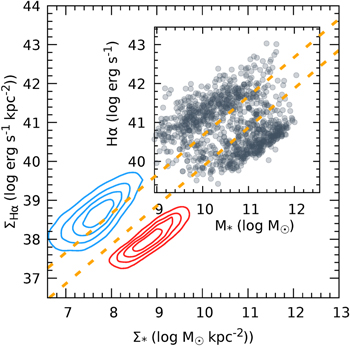
Figure 4. Resolved and global Hα and M* relation. In the main panel, the spatially resolved distribution is shown in contours. The blue and red contours indicate the distributions of the H ii spaxels in the star-forming galaxies and the LI(N)ER spaxels in the quiescent galaxies, respectively. The contour levels are 20%, 40%, 60%, and 80% of the peak density of the H ii or LI(N)ER spaxels. The two orange dashed lines are identical to the black dashed lines in Figure 1. The global distribution is shown as gray circles in the axis-aligned sub-panel. See the text for details.
Download figure:
Standard image High-resolution imageOn the other hand, the similarity between the resolved LI(N)ER sequence and the MPA-JHU global relation for the quiescent galaxies is rather surprising since the “SFR” in the latter catalog is calibrated using the relation between D4000 and SSFR based on emission-line galaxies.
4. Conclusion
In this Letter, we study the global and resolved Hα–M* relation for the MaNGA MPL-4 sample. We select star-forming and quiescent sequences with two constant SSFR criteria that consist of 960 isolated galaxies, and we analyze the distributions of the H ii and/or the LI(N)ER spaxels for both populations in the  –
– plot.
plot.
We conclude our results below:
(1) There is a tight  –
– correlation of the H ii spaxels for star-forming galaxies. The fitting results using the OLS method are consistent with Cano-Díaz et al. (2016).
(2) The H ii spaxels in quiescent galaxies have lower SSFR than those in star-forming galaxies, and the H ii fractions decrease toward the center region for quiescent galaxies with H ii fractions greater than 0.1. These results suggest that ∼20% of quiescent galaxies in our sample still have star formation activities in the outer region with lower SSFR than typical star-forming galaxies.
(3) The LI(N)ER spaxels in the quiescent galaxies show a tight  –
– correlation. This is the first time we show that the Hα emission is directly correlated with the underlying stellar mass surface density for regions classified as LI(N)ER. This can be consistent with the hot, evolved stars as the dominant mechanism powering the Hα emissions in quiescent galaxies.
(4) The global star-forming sequence is a continuous relation extended from the resolved  –
– relation. The remarkable agreement suggests that the global main sequence may originate from a more fundamental relation on small scales.
The work is supported by the Ministry of Science & Technology of Taiwan under grants MOST 103-2112-M-001-031-MY3 and 106-2112-M-001-034-. This project also makes use of the MaNGA-Pipe3D data products. We thank the IA-UNAM MaNGA team for creating it, and the ConaCyt-180125 project for supporting them. M.B. was supported by MINEDUC-UA project, code ANT 1655. R.R. thanks CNPq and FAPERGS for partial financial support.
Funding for the Sloan Digital Sky Survey IV has been provided by the Alfred P. Sloan Foundation, the U.S. Department of Energy Office of Science, and the Participating Institutions. SDSS-IV acknowledges support and resources from the Center for High-Performance Computing at the University of Utah. The SDSS web site is http://www.sdss.org. SDSS-IV is managed by the Astrophysical Research Consortium for the Participating Institutions of the SDSS Collaboration including the Brazilian Participation Group, the Carnegie Institution for Science, Carnegie Mellon University, the Chilean Participation Group, the French Participation Group, Harvard-Smithsonian Center for Astrophysics, Instituto de Astrofísica de Canarias, The Johns Hopkins University, Kavli Institute for the Physics and Mathematics of the Universe (IPMU)/University of Tokyo, Lawrence Berkeley National Laboratory, Leibniz Institut für Astrophysik Potsdam (AIP), Max-Planck-Institut für Astronomie (MPIA Heidelberg), Max-Planck-Institut für Astrophysik (MPA Garching), Max-Planck-Institut für Extraterrestrische Physik (MPE), National Astronomical Observatory of China, New Mexico State University, New York University, University of Notre Dame, Observatário Nacional/MCTI, The Ohio State University, Pennsylvania State University, Shanghai Astronomical Observatory, United Kingdom Participation Group, Universidad Nacional Autónoma de México, University of Arizona, University of Colorado Boulder, University of Oxford, University of Portsmouth, University of Utah, University of Virginia, University of Washington, University of Wisconsin, Vanderbilt University, and Yale University.