Abstract
Studies of close-in planets orbiting M dwarfs have suggested that the M-dwarf radius valley may be well explained by distinct formation timescales between enveloped terrestrials and rocky planets that form at late times in a gas-depleted environment. This scenario is at odds with the picture that close-in rocky planets form with a primordial gaseous envelope that is subsequently stripped away by some thermally driven mass-loss process. These two physical scenarios make unique predictions of the rocky/enveloped transition’s dependence on orbital separation such that studying the compositions of planets within the M-dwarf radius valley may be able to establish the dominant physics. Here, we present the discovery of one such keystone planet: the ultra-short-period planet TOI-1634 b (P = 0.989 days,  ,
,  R⊕) orbiting a nearby M2 dwarf (Ks = 8.7, Rs = 0.450 R⊙, Ms = 0.502 M⊙) and whose size and orbital period sit within the M-dwarf radius valley. We confirm the TESS-discovered planet candidate using extensive ground-based follow-up campaigns, including a set of 32 precise radial velocity measurements from HARPS-N. We measure a planetary mass of
  M⊕, which makes TOI-1634 b inconsistent with an Earth-like composition at
  and thus requires either an extended gaseous envelope, a large volatile-rich layer, or a rocky composition that is not dominated by iron and silicates to explain its mass and radius. The discovery that the bulk composition of TOI-1634 b is inconsistent with that of Earth supports the gas-depleted formation mechanism to explain the emergence of the radius valley around M dwarfs with
  M⊙.
M⊙.
1. Introduction
Early- to mid-M dwarfs experience extended pre-main-sequence lifetimes in which they remain XUV active for hundreds of Myr up to about a Gyr (Shkolnik & Barman 2014; France et al. 2016). This does not bode well for the survival of primordial H/He envelopes around close-in planets due to the envelope’s susceptibility to hydrodynamic escape driven by photoevaporation (e.g., Owen & Wu 2013; Jin et al. 2014; Lopez & Fortney 2014; Chen & Rogers 2016; Jin & Mordasini 2018) or by internal heating (i.e., core-powered mass loss; Ginzburg et al. 2018; Gupta & Schlichting 2019). In such scenarios, the largest rocky planets without envelopes increase toward greater insolation because planets need to be more massive to retain their envelopes. However, occurrence rate studies of close-in M-dwarf planets have revealed evidence that thermally driven mass loss does not sculpt the close-in M-dwarf planet population (Cloutier & Menou 2020) and instead, close-in gas-enveloped terrestrials and rocky planets formed on distinct timescales, with the latter forming at late times in a nearly gas-depleted environment (Lopez & Rice 2018). In this scenario, a natural outcome of terrestrial planet formation posits that the maximum radius of rocky planets increases toward lower insolation, in opposition to predictions from thermally driven mass loss. Because the thermally driven mass-loss and gas-depleted formation models make unique predictions regarding the location of the M-dwarf radius valley as a function of insolation or period, studying the bulk compositions of planets within the radius valley may be able to establish the dominant physics that sculpts the close-in planet population around M dwarfs.
Since its science operations began in 2018 July, NASA’s Transiting Exoplanet Survey Satellite (TESS; Ricker et al. 2015) has uncovered a wealth of transiting planet candidates whose orbital periods and radii lie within the radius valley, including three planets transiting early M dwarfs (TOI-1235 b; Bluhm et al. 2020; Cloutier et al. 2020b, TOI-776 b; Luque et al. 2021, TOI-1685 b; Bluhm et al. 2021). Radius valley planets whose periods P and radii rp satisfy
(Cloutier & Menou 2020) are referred to as keystone planets and are valuable targets to conduct tests of the competing radius valley emergence models across a range of stellar masses. Doing so requires that we characterize the bulk compositions of a sample of keystone planets using precise radial velocity (RV) measurements. Here we present the confirmation and characterization of one such keystone planet from TESS: TOI-1634 b. Our study focuses on the validation of the planet TOI-1634 b, including the recovery of its mass, and the implications that our results have on the emergence of the radius valley around early M dwarfs.
In Section 2 we present the properties of the host star TOI-1634. In Section 3 we present the TESS light curve and our suite of follow-up observations, which we use to validate the planetary nature of the planet candidate. In Section 4 we present our global data analysis and its results. We conclude with a discussion and a summary of our findings in Sections 5 and 6.
2. Stellar Characterization
Table 1 reports our adopted stellar parameters.
Table 1. TOI-1634 Stellar Parameters
| Parameter | Value | Refs |
|---|---|---|
| TOI-1634, TIC 201186294, 2MASS J03453363+3706438, | ||
| Gaia DR3 223158499179138432 | ||
| Astrometry | ||
| R.A. (J2015.5), α | 03:45:33.75 | 1, 2 |
| Decl. (J2015.5), δ | +37:06:44.21 | 1, 2 |
R.A. proper motion,  (mas yr−1) (mas yr−1) | 81.35 ± 0.02 | 1,2 |
Decl. proper motion,  (mas yr−1) (mas yr−1) | 13.55 ± 0.02 | 1,2 |
| Parallax, π (mas) | 28.512 ± 0.018 | 1, 2 |
| Distance, d (pc) | 35.274 ± 0.053 | 3 |
| (Uncontaminated) Photometry | ||
| V | 13.24 ± 0.04 | 4 |

| 13.5039 ± 0.0011 | 1, 6 |
| G | 12.1863 ± 0.0003 | 1, 6 |

| 11.0447 ± 0.0005 | 1, 6 |
| T | 11.0136 ± 0.0073 | 7 |
| J | 9.564 ± 0.021 | 4 |
| H | 8.940 ± 0.021 | 4 |
| Ks | 8.699 ± 0.014 | 4 |
| W1 | 8.429 ± 0.022 | 5 |
| W2 | 8.325 ± 0.020 | 5 |
| W3 | 8.250 ± 0.023 | 5 |
| W4 | 8.266 ± 0.300 | 5 |
| Stellar parameters | ||
| Spectral type | M2 | 4 |

| 5.88 ± 0.01 | 4 |
Effective temperature,  (K) (K) | 3550 ± 69 | 4 |
| Surface gravity, log g (dex) | 4.833 ± 0.028 | 4 |
| Metallicity, [Fe/H] (dex) |

| 4 |
| Stellar radius, Rs (R⊙) | 0.450 ± 0.013 | 4 |
| Stellar mass, Ms (M⊙) | 0.502 ± 0.014 | 4 |
Stellar density,  (g cm−3) (g cm−3) |

| 4 |
Stellar luminosity, Ls
(
|

| 4 |
| Projected rotation velocity, | ||
| <1.3 a | 4 | |
 (km s−1) (km s−1) | ||

| −5.39 ± 0.19 | 4 |
Rotation period,  (days)
b (days)
b
|

| 4 |
References. (1) Gaia Collaboration et al. (2021) (2) Lindegren et al. (2021) (3) Bailer-Jones et al. (2018) (4) this work (5) Cutri (2014) (6) Riello et al. (2021) (7) Stassun et al. (2019).
a Based on the upper limits on rotational broadening from the cross-correlation function of our HARPS-N spectra. b We do not measure the stellar rotation period. Rather, is estimated from the rotation–activity relation of Astudillo-Defru et al. (2017).
Download table as: ASCIITypeset image
TOI-1634 (TIC 201186294, 2MASS J03453363+3706438, Gaia DR3 223158499179138432) is an M2 dwarf (Pecaut & Mamajek 2013) at a distance of 35.274 ± 0.053 pc (Bailer-Jones et al. 2018; Gaia Collaboration et al. 2021; Lindegren et al. 2021). The value of the Gaia EDR3 RUWE (renormalized unit weight error) astrometric quality indicator reveals that TOI-1634's astrometric solution shows a large excess of 0.121 mas
44
This may be indicative of a long-period companion to TOI-1634, which we will revisit with our follow-up observations in Sections 3.5 and 3.6. Gaia EDR3 also revealed a faint ( mag) comoving companion at 2
69 west of TOI-1634 at a projected separation of 94.1 au (i.e., TIC 641991121, Gaia DR3 223158499176634112; Mugrauer & Michel 2020). This source is clearly resolved by Gaia such that it cannot be responsible for the excess noise in TOI-1634's astrometric solution. The companion does not appear in the 2MASS Point Source Catalog (Cutri et al. 2003). Consequently, the 2MASS blend and contamination/confusion flags for TOI-1634 (bb_flg, cc_flg) indicate that its photometry was fit by a single source as it was assumed to be uncontaminated. Similar issues of uncorrected contamination persist for TOI-1634 in all but the Gaia passbands. To infer stellar parameters from empirical relations, we correct TOI-1634's V-band and 2MASS photometry using each source’s Gaia photometry and computing their magnitude differences in VJHKS
using appropriate Gaia color relations (Evans et al. 2018). We derive Δmag correction factors of 0.021, 0.080, 0.093, and 0.099 in the VJHKS
bands, respectively.
The refined 2MASS photometry for TOI-1634 has critical consequences for the derivation of its global stellar properties from empirical relations. Using the M-dwarf KS
-band mass–luminosity relation from Benedict et al. (2016), we find that  M⊙. This value is
  discrepant from the result obtained without correcting the KS
-band magnitude. Similarly, we measure a stellar radius of
discrepant from the result obtained without correcting the KS
-band magnitude. Similarly, we measure a stellar radius of  R⊙ using the M-dwarf radius–luminosity relation from Mann et al. (2015). Together, these yield
  . We derive the stellar effective temperature of
  K using the uncontaminated Gaia photometry and the
  ) relation from Mann et al. (2015). We also estimate the stellar metallicity using the empirical
 ![$(V-{K}_{S})\,-{M}_{{K}_{S}}-[\mathrm{Fe}/{\rm{H}}]$](https://content.cld.iop.org/journals/1538-3881/162/2/79/revision1/ajac0157ieqn29.gif) relation for M dwarfs from Johnson & Apps (2009). We find a somewhat metal-rich value of
relation for M dwarfs from Johnson & Apps (2009). We find a somewhat metal-rich value of ![$[\mathrm{Fe}/{\rm{H}}]\,={0.23}_{-0.08}^{+0.07}$](https://content.cld.iop.org/journals/1538-3881/162/2/79/revision1/ajac0157ieqn30.gif) dex, consistent with suggested correlations for low-mass stars between metallicity and the presence of small planets (e.g., Johnson & Apps 2009; Schlaufman & Laughlin 2011).
dex, consistent with suggested correlations for low-mass stars between metallicity and the presence of small planets (e.g., Johnson & Apps 2009; Schlaufman & Laughlin 2011).
The companion star is in version 8 of the TESS Input Catalog (TIC; Stassun et al. 2019), with its TESS magnitude (T = 14.37 mag) estimated solely from Gaia photometry. We analyzed the spectral energy distributions (SEDs) of both stars to refine the dilution of TOI-1634 in the TESS band. Due to the flux contamination, we performed a two-component fit following the procedures outlined in Stassun & Torres (2016, 2018) and Stassun et al. (2017). For TOI-1634, we use the JHKS
magnitudes from 2MASS, W1–W4 from WISE, and Gaia  magnitudes. For the companion we use the ui bands from SDSS, the y band from Pan-STARRS, and Gaia
  magnitudes (see Figure 1). We fit for
  and [Fe/H] in each SED using a NextGen stellar atmosphere model (Hauschildt et al. 1999) with zero extinction (AV
= 0). After correcting TOI-1634's SED for the flux of the companion, we measure
and [Fe/H] in each SED using a NextGen stellar atmosphere model (Hauschildt et al. 1999) with zero extinction (AV
= 0). After correcting TOI-1634's SED for the flux of the companion, we measure  K and
K and ![$[\mathrm{Fe}/{\rm{H}}]=0.0\pm 0.5$](https://content.cld.iop.org/journals/1538-3881/162/2/79/revision1/ajac0157ieqn35.gif) dex, both of which are consistent with the values derived from empirical relations. Similarly for the companion star, we measure
dex, both of which are consistent with the values derived from empirical relations. Similarly for the companion star, we measure  K and
K and ![${[\mathrm{Fe}/{\rm{H}}]}_{\mathrm{comp}}=0.0\,\pm 0.5$](https://content.cld.iop.org/journals/1538-3881/162/2/79/revision1/ajac0157ieqn37.gif) dex. Integrating the SED at a distance of 35.274 pc yields a bolometric flux at Earth of
dex. Integrating the SED at a distance of 35.274 pc yields a bolometric flux at Earth of  erg s−1 cm−2, which corresponds to
  R⊙ and again is consistent with the value derived from the empirical radius–luminosity relation. Given the total fluxes from our SED analysis, we recover a dilution factor of
  , which is consistent with the original value of 0.943 used by the NASA Ames Science Processing Operations Center when producing the TESS light curve (see Section 3.1). Our derived dilution factor ignores the two remaining sources that sit within the TESS aperture due to their negligible flux contributions (see Figure 2).
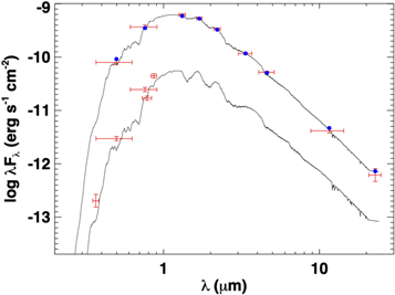
Figure 1. The spectral energy distributions of the target star TOI-1634 and its faint companion. The black curves depict the stellar atmosphere models for each star with effective temperatures of 3500 K and 3025 K, respectively. The red markers depict the photometric measurements and their uncertainties. The horizontal error bars depict the effective width of each passband. The blue markers depict the model flux in each passband for TOI-1634.
Download figure:
Standard image High-resolution image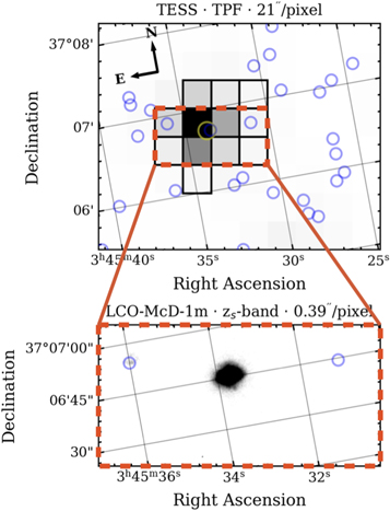
Figure 2. Images of the field surrounding TOI-1634. Upper panel: a sample TESS target pixel file image of TOI-1634 with a pixel scale of  . The yellow circle highlights TOI-1634 while the blue markers highlight its nearby stellar companion and other neighboring sources from Gaia EDR3. The pixels outlined in black demarcate the TESS photometric aperture used to produce the PDCSAP light curve of TOI-1634. Lower panel: a zoom in on the highlighted red region taken with the LCOGT 1 m telescope at McDonald Observatory with a pixel scale of
  . The small angular separation between TOI-1634 and its companion prevents the source from being spatially resolved in our seeing-limited images.
Download figure:
Standard image High-resolution imageThe photometric stellar rotation period is presently unknown (see Section 3.2). We establish a prior on  using the empirical M-dwarf rotation–activity relation from Astudillo-Defru et al. (2017). From our HARPS-N spectra presented in Section 3.6, we measure
  , which places TOI-1634 within the unsaturated regime of magnetic activity (e.g., Reiners et al. 2009). Using the rotation–activity relation for inactive M dwarfs, we estimate
  days. Such a long rotation period would place TOI-1634 in the long-period tail of the
  distribution among M dwarfs with masses between 0.4 and 0.6 M⊙ (10–70 days; Newton et al. 2017).
3. Observations
3.1. TESS Photometry
TOI-1634 was observed by TESS for 24.38 days from UT 2019 November 3–27 in Sector 18. The observations were taken with CCD 4 on camera 1. TOI-1634 is not slated for further observations with TESS. 45 TOI-1634 is listed in v8 of the TESS Input Catalog, the Candidate Target List (CTL), and as a target in the Guest Investigator program G022198 46 such that it was observed with 2 minute cadence. A total of 20 transits were observed with three transit events being missed during the data transfer event near perigee passage.
A sample image from the TESS target pixel files (TPFs) is shown in the upper panel of Figure 2 overlaid by a subset of the 78 Gaia sources within  . All image data were processed by the NASA Ames Science Processing Operations Center (SPOC; Jenkins et al. 2016), which then proceeded to produce the Presearch Data Conditioning Simple Aperture Photometry (PDCSAP; Smith et al. 2012; Stumpe et al. 2012, 2014) light curve using the 12 pixel photometric aperture overlaid in Figure 2. The aperture clearly contains contributions from TOI-1634, its nearby stellar companion, and at least two faint background sources from Gaia. TOI-1634 dominates the flux within the aperture and contributes 0.943 of the flux to the PDCSAP light curve on average.
Late in the primary mission, the SPOC identified a bias in the background sky correction that shifts the PDCSAP light curve to lower flux values. Following the instructions outlined in the Sector 27 release notes,
47
we correct this effect by determining the background bias 
 /s/pixel from the difference between the background-corrected pixel fluxes and zero. We then correct the PDCSAP flux according to

where  is the number of pixels in the optimal aperture and CROWDSAP/FLFRCSAP = 1.14 is the ratio of the crowding metric to the flux fraction correction, which are provided in the SPOC light-curve fits headers. This correction adjusts the baseline flux and hence decreases the inferred transit depth, by 2.2%.
The dilution and background-corrected PDCSAP light curve for TOI-1634 is shown in the upper panel of Figure 3 with the 20 transits of TOI-1634.01 highlighted in green. Note that no obvious signature of stellar rotation is apparent in the light curve. It is on these data that the SPOC conducted its transit search using the Transiting Planet Search Pipeline Module (TPS; Jenkins 2002; Jenkins et al. 2010). After passing a set of internal data validation tests (Twicken et al. 2018; Li et al. 2019), the TPS returned the new transiting planet candidate TOI-1634.01 with an orbital period of 0.989 days and a transit depth of 1.52 ± 0.13 ppt. Using the stellar radius from Table 1, this initial transit depth corresponds to a planet radius of 1.90 ± 0.10 R⊕. The public release of the candidate TOI-1634.01 in 2019 December prompted our follow-up observations described in Sections 3.3–3.6.
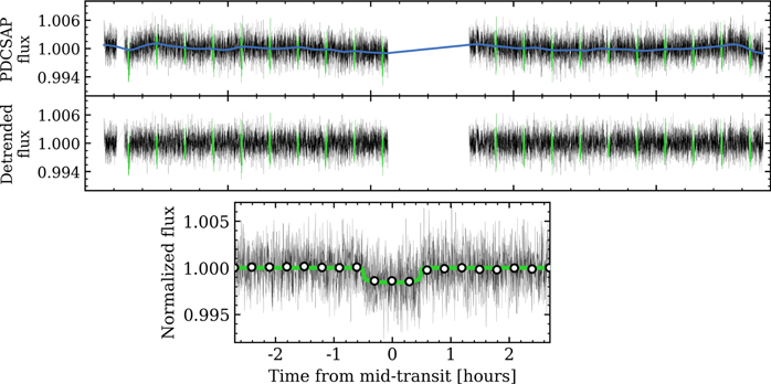
Figure 3. TESS PDCSAP light curve of TOI-1634 from Sector 18. Top panel: the dilution and background-corrected PDCSAP light curve overlaid with the mean GP model of residual correlated noise (blue curve). In-transit measurements are highlighted in green. Middle panel: the PDCSAP light curve detrended by the mean GP model. Bottom panel: the phase-folded transit light curve of TOI-1634 b. The maximum a posteriori transit model is overlaid in green while the white markers depict the binned light curve.
Download figure:
Standard image High-resolution image3.2. Archival Photometric Monitoring
Recall that the TESS light curve does not show any signs of rotation (Figure 3). This is consistent with TOI-1634 being relatively inactive given its low value of  and the expectation of a long rotation period of
  days. Furthermore, we cannot hope to obtain a precise
  measurement with just one TESS sector if indeed
  is as long as we expect (Lu et al. 2020).
We attempt to recover  by investigating the long-baseline archival photometric monitoring from the ASAS-SN survey (Jayasinghe et al. 2019). The ASAS-SN survey monitored TOI-1634 from 2012 November to 2020 October in the V and g bands. Figure 4 shows the light curves and their generalized Lomb–Scargle periodograms (GLS; Zechmeister & Kürster 2009). We compute the false-alarm probability (FAP) for each GLS periodogram via bootstrapping with replacement. We inspected the periodogram of each light curve and found no coherent periodic signal that is present in both light curves. Most notably, there is no persistent signal over the domain between 50 and 105 days where we expect to measure
  for TOI-1634 based on its
  value.
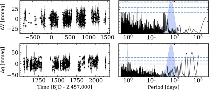
Figure 4. Photometric monitoring of TOI-1634 with ASAS-SN in the V band (upper row) and g band (lower row). Left column: differential light curves. Right column: the GLS periodograms of each light curve. The blue histogram depicts the expected stellar rotation period based on the star’s  and the rotation–activity relation from Astudillo-Defru et al. (2017). The horizontal dashed lines depict FAPs of 0.1%, 1%, and 10%. No coherent periodic signal is detected.
Download figure:
Standard image High-resolution image3.3. Reconnaissance Spectroscopy with TRES
Through the TESS Follow-up Observing Program (TFOP), we began to pursue the confirmation of the planet candidate TOI-1634.01 by obtaining a pair of reconnaissance spectra. We observed TOI-1634 on UT 2020 February 2 and 2020 September 5 using the Tillinghast Reflector Échelle Spectrograph (TRES). TRES is a fiber-fed optical échelle spectrograph (310–910 nm) with a resolution of R = 44,000 and is mounted on the 1.5 m Tillinghast Reflector telescope at the Fred Lawrence Whipple Observatory on Mount Hopkins, Arizona. The exposure time was set to 3000 s. We reduced and extracted the spectra using the standard procedure (Buchhave et al. 2010) before cross-correlating the spectra with a custom spectral template of Barnard’s star that was rotationally broadened over a range of  values (Winters et al. 2018). We selected the échelle aperture 41 between 7065 and 7165 Å for RV extraction as it contains the information-rich TiO bands. We estimate the corresponding RV precision at each epoch to be 65 and 38 m s−1.
We find TOI-1634 to be single lined with no significant rotational broadening ( < 3.4 m s−1), and with the
  feature in absorption (Figure A1). Our two TRES observations were also scheduled at opposing quadrature phases and revealed no large RV variation beyond the level of our RV uncertainties. These data confirm that TOI-1634 is a chromospherically inactive and slowly rotating star. These data also likely rule out the possibility of a spectroscopic binary such that TOI-1634.01 continues to be a viable planet candidate, and we can proceed with further attempts at planet confirmation.
3.4. Seeing-limited Photometry
TESS pixels are large ( ), which results in the blending of the TOI-1634 light curve with nearby sources. We therefore obtained seeing-limited photometry to confirm the transit on target and to spatially resolve the light curves of nearby sources to rule out nearby eclipsing binaries (NEBs) as the source of the TESS transit events. We obtained a total of 16 light curves of seven distinct transit events with a variety of observing facilities. Table 2 summarizes the observations with the individual facilities described in the following sections. The light curves are shown in Figure A2.
Table 2. Summary of Seeing-limited Photometric Follow-up of TOI-1634
| Obs. Date | Filter | Telescope | PSF FWHM | Photometric | Photometric |
|---|---|---|---|---|---|
| (YYYY MM DD) | Aperture (m) | (″) | Aperture (″) | Precision (ppt) a | |
| LCO McDonald | |||||
| 2020 Sep 30 | zs | 1.0 | 4.2 | 2.5 | 0.5 |
| MuSCAT2 | |||||
| 2020 Feb 7 |

| 1.52 | 1.9,1.8,1.8,1.7 | 4.0 | 2.6,0.9,1.0,0.8 |
| 2020 Feb 10 |

| 1.52 | 1.9,1.5,1.7,1.6 | 4.3 | 2.0,1.2,1.2,0.9 |
| 2020 Feb 11 |

| 1.52 | 1.8,1.5,1.6,1.2 | 4.3 | 1.6,1.1,0.8,0.8 |
| OAA | |||||
| 2020 Feb 13 | Ic | 0.40 | 5.5 | 10.0 | 1.3 |
| 2020 Feb 21 | Ic | 0.40 | 7.6 | 10.0 | 1.4 |
| RCO | |||||
| 2020 Feb 20 |

| 0.40 | 4.8 | 8.0 | 1.4 |
Note.
a Photometric precision is calculated as the rms of the detrended light curve in approximately 5 minute bins.Download table as: ASCIITypeset image
In summary, we successfully confirm the transit time of TOI-1634.01 and are able to rule out 38 of 39 sources within  as NEBs. However, the comoving companion to TOI-1634 at
  is unresolved in all of our observations (see lower panel of Figure 2). Even in our highest-quality ground-based light curves, at most 50% of the companion’s flux can be excluded from the photometric aperture. As such, these data cannot uniquely identify TOI-1634 as the host of the TESS transit events, although they do limit the possibilities to either TOI-1634 or its companion.
3.4.1. LCOGT
We observed a full transit of TOI-1634.01 on UT 2020 September 30 in the Pan-STARRS zs
band from the Las Cumbres Observatory Global Telescope (LCOGT; Brown et al. 2013) 1 m network node at McDonald Observatory. We used the TESS Transit Finder, which is a customized version of the Tapir software package (Jensen 2013), to schedule our transit observations. The 4096 × 4096 LCOGT SINISTRO cameras have an image scale of  per pixel, resulting in a
  field of view. The images were calibrated by the standard LCOGT BANZAI pipeline (McCully et al. 2018), and photometric data were extracted with AstroImageJ (Collins et al. 2017). The TOI-1634.01 observation used 40 second exposures and a photometric aperture radius of
  to extract the differential photometry.
3.4.2. MuSCAT2
MuSCAT2 (Narita et al. 2019) is a multicolor camera that is able to obtain simultaneous observations in four bands:
Sloan-g, Sloan
-r, Sloan-i, and Sloan-zs
. The instrument is mounted on the 1.52 m Telescopio Carlos Sánchez (TCS) at Teide Observatory, Tenerife, Spain. The field of view of MuSCAT2 is  with a pixel scale of
  per pixel. All the cameras have a short read-out time between 1 and 4 s, which makes MuSCAT2 an ideal instrument for transit follow-up and time-series observations in general. We observed three primary transits of TOI-1634 b in all four bands on the nights of UT 2020 February 7, 10, and 11. For each night, we set the exposure times to avoid the saturation of the target star. We reduced the data using standard procedures: the photometry and transit model fit (including systematic effects) was done by the MuSCAT2 pipeline (Parviainen et al. 2019, 2020).
3.4.3. OAA
We observed two full transits of TOI-1634.01 on UT 2020 February 13 and 21 using the main 0.4 m instrument ensemble at Observatori Astronòmic Albanyà (OAA) with stable observation conditions in the valley. We performed differential photometry in a  star field centered on TOI-1634 using the Ic
filter with
star field centered on TOI-1634 using the Ic
filter with  photometric apertures (in
  FWHM conditions) using the AstroImageJ pipeline. The sequences consisted of 88 and 148 frames of 120 s and 100 s exposure times, respectively. A small number of outlying points during transit due to instrumental inconveniences (>10σ) were removed before the transit fit. No significant NEB signals were detected within
  of the target after performing a thorough NEB check with different apertures from 4
5 to 10
0.
3.4.4. RCO
A full transit observation of TOI-1634.01 was obtained on UT 2020 February 20 using the RCO 40 cm telescope located at the Grand-Pra Observatory, Switzerland. We observed a full transit in the Sloan-i′ passband with an exposure time of 90 s. We produced the light curve of TOI-1634.01 using the AstroImageJ pipeline with  apertures and by detrending against airmass and FWHM. We confirmed that no NEB signals appeared at the expected time within
  of TOI-1634.
3.5. High-resolution Imaging
The smallest PSF of our seeing-limited photometric observations has an FWHM of  . Thus, with seeing-limited photometry alone, we are insensitive to sources more closely separated from TOI-1634 than approximately this limit. To check for blended sources within
  , we obtained four sets of high-resolution imaging sequences (Figure A3), which are described in the following subsections. Other than the known stellar companion at
  separation, we do not find evidence for any additional contaminating sources down to
  given the sensitivity of our observations and thus do not find any supporting evidence for a massive long-period companion that may have been able to account for TOI-1634's excess astrometric noise in Gaia EDR3. As such, TOI-1634.01 remains a viable planet candidate.
3.5.1. ’Alopeke
We obtained speckle interferometric images of TOI-1634 on UT 2020 February 16 using the ’Alopeke instrument
48
mounted on the 8 m Gemini North telescope on the summit of Maunakea in Hawai’i. ’Alopeke simultaneously collects diffraction-limited images at 562 and 832 nm. Our data set consists of 7 minutes of total integration time taken as sets of  images. Following Howell et al. (2011), we combined all images, subjected them to Fourier analysis, and produced reconstructed images from which the 5σ contrast curves are derived in each passband. Figure A3 presents the two contrast curves as well as the 832 nm reconstructed image. Our measurements reveal TOI-1634 to be a single star down to Δmag 5–7, eliminating all main-sequence stellar companions earlier than M6 within the spatial limits of 0.6–1.0 au at the inner working angle, and out to 42 au at
  .
.
3.5.2. ShARCS
We observed TOI-1634 on UT 2020 December 1 using the ShARCS camera on the Shane 3 m telescope at Lick Observatory. Our observations were taken using the Shane adaptive optics (AO) system in natural guide star mode. We collected our observations using a four-point dither pattern with a separation of  between each dither position. We obtained a pair of sequences; in the J and KS
bands with exposure times of 7.5 s and 15 s, respectively. See Savel et al. (2020) for a detailed description of the observing strategy and reduction procedure. Our AO images and contrast curves for each imaging sequence are shown in Figure A3. We detect the known companion but find no other nearby companions within
between each dither position. We obtained a pair of sequences; in the J and KS
bands with exposure times of 7.5 s and 15 s, respectively. See Savel et al. (2020) for a detailed description of the observing strategy and reduction procedure. Our AO images and contrast curves for each imaging sequence are shown in Figure A3. We detect the known companion but find no other nearby companions within  down to
  mag and
  mag.
mag.
3.6. Precise Radial Velocity Measurements
We obtained 32 spectra of TOI-1634 using the HARPS-N spectrograph located at the 3.6 m Telescopio Nazionale Galileo (TNG) on La Palma, Canary Islands. HARPS-N is a high-resolution (R = 115,000) optical échelle spectrograph whose long-term pressure and temperature stability enable it to reach sub-meter-per-second stability (Cosentino et al. 2012). The exposure time was fixed to 1800 s. We follow the standard procedure for M-dwarf observations with HARPS-N and focus solely on the échelle orders redward of aperture 18 (i.e., 440–687 nm; Anglada-Escudé & Butler 2012). The median total signal-to-noise ratio (S/N) of our spectra is 107.
We obtained our observations over a 210 day span between UT 2020 August 7 and 2021 March 4 as part of the HARPS-N collaboration Guaranteed Time Observations. Due to the proximity of TOI-1634.01's orbital period to 1 day (P = 0.989 days), we were unable to obtain uniform sampling of the planet’s orbital phase. Fortunately, the combination of the planet’s ephemeris and the longitude of the TNG observatory resulted in a preferential sampling of the planet’s orbit near its quadrature phases (i.e., ϕ ∼ ±0.25). The information content of our time series with respect to the RV semiamplitude is much richer than if only orbital phases close to 0 and 0.5 could be sampled. However, although this restricted sampling had only a small effect on the inference of the planet’s RV semiamplitude from preliminary analyses, we found that the constraints on the orbital eccentricity were very weak when left unconstrained. Note that given the planet’s ultra-short period (USP), it is reasonable to expect a circularized orbit with little to no eccentricity (see Section 5.1). To remedy the lack of observational constraints on orbital eccentricity, the six most recent RV measurements were intentionally scheduled to fill in the gaps in our orbital phase sampling in an effort to distinguish between circular and eccentric orbital solutions.
We extracted the RVs via template-matching using the TERRA pipeline (Anglada-Escudé & Butler 2012). Template-matching is a commonly used tool for the RV extraction from M-dwarf spectra as it is known to achieve improved RV precision over the more traditional cross-correlation function techniques (e.g., Astudillo-Defru et al. 2015). TERRA works by constructing a master template spectrum by coadding all of the individual spectra after shifting each spectrum to the barycentric frame. The barycentric corrections are retrieved from the HARPS-N Data Reduction Software (DRS; Lovis & Pepe 2007). We ignore spectral regions in which the telluric absorption exceeds 1%. The RV of each spectrum is then calculated via least-squares matching of the spectrum to the master template in velocity space. Due to the poor S/N of the bluest orders, we only focus on échelle orders redward of aperture 18. We obtain a median RV uncertainty of 1.73 m s−1.
Figure 5 shows the GLS periodograms of the RVs, the window function, and the following activity indicators produced by the DRS: CCF FWHM, CCF BIS, Hα ( ), and both sodium doublet features Na D1 (
 ) and Na D2 (
 ). We do not observe any significant periodic signals in any of the activity indicators, thus we do not recover the stellar rotation period from these spectroscopic indicators. The only significant (FAP < 1%) persistent signal that emerges in multiple time series is close to 1 day, which we expect in the RVs due to the transiting planet candidate with P = 0.989 days (also shown zoomed-in in Figure 6). The 1 day signal is also apparent in the window function due to the effect of the one-day alias—a phenomenon that often inhibits the detection of periodic RV signals close to one day (Dawson & Fabrycky 2010) but is not a major issue in our analysis due to the strong prior on the planet’s orbital period from the transit data. The time series depicted in Figure 5 are provided in Table 3.
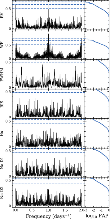
Figure 5. GLS periodograms of the HARPS-N RVs, window function (WF), and spectroscopic indicators of TOI-1634. Left column: the GLS periodogram of the time series labeled on the y-axis. The horizontal dashed lines report the FAP levels of 0.1%, 1%, and 10%. Right column: the FAP as a function of normalized power.
Download figure:
Standard image High-resolution image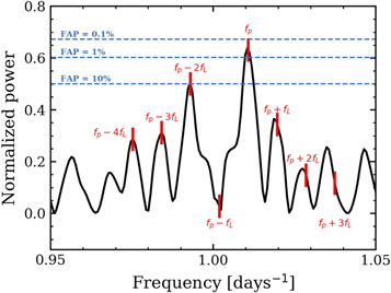
Figure 6. The GLS periodogram of the TOI-1634 RVs in the vicinity of the planet candidate’s orbital frequency  day−1. The forest of peaks can be well explained as aliasing by the long period frequency
  day−1 seen in the RVs. The horizontal dashed lines report the FAP levels of 0.1%, 1%, and 10%.
Download figure:
Standard image High-resolution imageTable 3. HARPS-N Time Series of TOI-1634
| Time | RV |

| FWHM | BIS | Hα | Na D1 | Na D2 |
|---|---|---|---|---|---|---|---|
| (BJD-2,457,000) |

|

|

|

| |||
| 2068.720217 | −0.246 | 1.753 | 3.064 | −12.248 | 0.911 | 0.486 | 0.613 |
| 2069.716163 | −6.512 | 2.427 | 2.974 | −6.289 | 0.892 | 0.472 | 0.627 |
| 2070.717423 | −6.615 | 1.572 | 2.989 | 4.337 | 0.879 | 0.441 | 0.585 |
Only a portion of this table is shown here to demonstrate its form and content. A machine-readable version of the full table is available.
Download table as: DataTypeset image
One remaining low FAP signal is seen solely in the RVs at a frequency of  day−1. The origin of the 113 day signal is unlikely to be due to stellar rotation as the signal is not visible in any of the activity indicators, and it would represent an uncharacteristically long rotation period for an inactive M dwarf with the mass of TOI-1634. The signal may also potentially be due to the long-period companion that was posited based on the excess noise in the Gaia EDR3 astrometry (Section 2). However, Figure 6 reveals that the 113 day signal (i.e.,
  day−1) is an alias as it can explain the forest of peaks aliasing the planet candidate at the frequencies
  , where
  day−1 is the orbital frequency of TOI-1634.01 and n takes on integer values. In Section 4.2 we will confirm that the 113 day signal is a spurious aliased signal that disappears upon the removal of the signal at fp
.
day−1 is the orbital frequency of TOI-1634.01 and n takes on integer values. In Section 4.2 we will confirm that the 113 day signal is a spurious aliased signal that disappears upon the removal of the signal at fp
.
4. Transit Plus RV Analysis and Results
We proceed with measuring the accessible planetary parameters following a two-step process. We first model the TESS transit light curve alone to remove any residual low-order systematics and to derive initial estimates of the transit parameters (Section 4.1). We then use those initializations to produce a global transit plus RV model from which we measure the physical and orbital properties of TOI-1634 b (Section 4.2).
4.1. TESS Transit Analysis
Standard systematics detrending has already been applied to the TESS PDCSAP photometry by the SPOC. However, some low-amplitude variability is seen to persist, which we attribute to residual systematics (top panel of Figure 3). Here we model the PDCSAP light curve with a transiting planet model plus systematics model in the form of an untrained Gaussian process (GP). The covariance of the GP is parameterized as a stochastically driven simple harmonic oscillator in Fourier space, which enables efficient computations of the GP’s marginalized likelihood when operating on large data sets (i.e., when a number of data points ≫ a number of model parameters). The spectral density of the covariance kernel is

where  is the frequency of the undamped oscillator and S0 describes the spectral power at
  . We also include an additive scalar jitter term to account for any excess uncorrelated noise in the TESS photometry:
  . The simultaneous Mandel & Agol (2002) transit model has the following free parameters: stellar mass Ms
, stellar radius Rs
, quadratic limb-darkening coefficients
. The simultaneous Mandel & Agol (2002) transit model has the following free parameters: stellar mass Ms
, stellar radius Rs
, quadratic limb-darkening coefficients  , orbital period P, time of midtransit b, eccentricity e, argument of periastron
  , and flux baseline f0
. We include samples of MT0, planet radius rp
, impact parameters s and Rs
as, together with P, they uniquely constrain the scaled semimajor axis
, and flux baseline f0
. We include samples of MT0, planet radius rp
, impact parameters s and Rs
as, together with P, they uniquely constrain the scaled semimajor axis  and the stellar density, which in turn constrains permissible values of e and
  (Moorhead et al. 2011; Dawson & Johnson 2012). Our full model features 14 model parameters with the following parameterizations:
 . The respective priors are listed in Table 4.
Table 4. TESS Light Curve and RV Model Parameter Priors
| Parameter | Fiducial Model Priors |
|---|---|
| Stellar parameters | |
| Ms (M⊙) |

|
| Rs (R⊙) |

|
| Light-curve hyperparameters | |

|

|
 (day−1) (day−1) |

|

|
|

|
 a
a
|

|

|

|

|
| RV parameters | |
 (m s−1) (m s−1) |

|
 (m s−1) (m s−1) |

|
| TOI-1634 b parameters | |
| P (days) |

|
| T0 (BJD-2,457,000) |

|
 (R⊕) (R⊕) |
 b
b
|

|

|
| b |

|
 (m s−1) (m s−1) |

|
| e |
 c
c
|
| ω (rad) |
 c
c
|

|

|

|

|
Notes. Gaussian distributions are denoted by  and are parameterized by the mean and standard deviation values. Uniform distributions are denoted by
  and bounded by the specified lower and upper limits. Beta distributions are denoted by
  and are parameterized by the shape parameters α and β.
 is the flux time series representing the dilution and background-corrected PDCSAP light curve from TESS.
b
The transit depth of TOI-1634.01 reported by the SPOC: Z = 1520 ppm.
c
For use in the TESS analysis only (Kipping 2013).
is the flux time series representing the dilution and background-corrected PDCSAP light curve from TESS.
b
The transit depth of TOI-1634.01 reported by the SPOC: Z = 1520 ppm.
c
For use in the TESS analysis only (Kipping 2013).Download table as: ASCIITypeset image
We use PyMC3 (Salvatier et al. 2016) within the exoplanet package (Foreman-Mackey et al. 2019) to evaluate the model’s joint posterior via Markov Chain Monte Carlo (MCMC). Within exoplanet, the separate software packages celerite (Foreman-Mackey et al. 2017) and STARRY (Luger et al. 2019) are used to calculate the GP and transit models, respectively. We run four simultaneous chains with 4000 tuning steps to derive the model’s joint posterior. We use the maximum a posteriori (MAP) point estimates of the GP hyperparameters to construct the GP posterior (i.e., predictive) distribution whose mean function we use to detrend the TESS photometry (middle panel of Figure 3). We then adopt the MAP transit model parameters to initialize the MCMC of our global model in the next section.
4.2. Global Modeling
We proceed with constructing our global model, which jointly considers the transit and RV data sets. The primary purpose of our seeing-limited photometric observations (Section 3.4) was to rule out neighboring sources as the origin of the TESS transit events (i.e., NEBs). This purpose has been successfully served so there is no need to include all of those observations in our global model. Instead, here we only include the most recent high S/N observation from LCOGT in the zs band. This choice provides the longest time baseline and thus provides the strongest constraints on the planet’s ephemeris.
Even inactive M dwarfs rotate and exhibit some level of magnetic activity. However, our photometric and spectroscopic analyses have indicated that TOI-1634 shows no evidence for coherent and temporally sustained signals from stellar activity. As such, in our fiducial model, we do not attempt to model any temporal correlations from stellar activity and simply model excess jitter with an additive scalar term  . Our fiducial transit plus RV model therefore features a total of 16 parameters. Among these are the same transit model parameters described in Section 4.1, with the exception of the GP hyperparameters as here we consider the detrended TESS light curve. However, we modify the parameterization of rp
, e, and
. Our fiducial transit plus RV model therefore features a total of 16 parameters. Among these are the same transit model parameters described in Section 4.1, with the exception of the GP hyperparameters as here we consider the detrended TESS light curve. However, we modify the parameterization of rp
, e, and  as follows. The planet radius rp
becomes the planet-to-star ratio
as follows. The planet radius rp
becomes the planet-to-star ratio  , which has a unique index i for each passband
 ![$\in [T,{z}_{s}]$](https://content.cld.iop.org/journals/1538-3881/162/2/79/revision1/ajac0157ieqn153.gif) . Similarly, each passband has a unique flux baseline
. Similarly, each passband has a unique flux baseline  . The zs
limb-darkening coefficients were fixed to
. The zs
limb-darkening coefficients were fixed to  and
and  (Claret & Bloemen 2011). To avoid the Lucy–Sweeney bias against e = 0, we elect to sample the parameters
  and
and  (Lucy & Sweeney 1971; Eastman et al. 2013).
49
The RV component of our model then consists of three additional parameters: the RV semiamplitude K, the velocity offset
(Lucy & Sweeney 1971; Eastman et al. 2013).
49
The RV component of our model then consists of three additional parameters: the RV semiamplitude K, the velocity offset  , and the aforementioned additive scalar jitter
  . Our complete set of model parameters is
 . Their respective priors are also listed in Table 4.
Given that the Gaia EDR3 astrometric solution may be consistent with the existence of a long-period companion, we also considered an RV model that includes a linear trend term. We determine that the slope of the linear trend is consistent with zero, thus indicating that our RV data are able to strongly rule out a long-period companion out to approximately the baseline of our observations (i.e., 210 days).
We fit the TESS, LCO, and HARPS-N RV data with our fiducial model and sample the joint posterior using the affine-invariant ensemble MCMC sampler emcee (Foreman-Mackey et al. 2013). We initialize 200 walkers and evaluate the convergence of each walker’s chain by insisting that  autocorrelation times are sampled. MAP point estimates of the model parameters are derived from their respective marginalized posteriors and are reported in Table 5 along with uncertainties derived from the 16th and 84th percentiles. The resulting transit model is shown in the lower panel of Figure 3 while the RV results are shown in Figure 7. The Keplerian RV signal from TOI-1634 b is clearly detected with a semiamplitude of
  m s−1 and on an orbit that is consistent with circular (i.e.,
  at 95% confidence). The 113 day signal in the RVs disappears with the subtraction of the planet model, which supports the notion that the signal was merely an alias rather than physical.
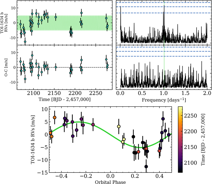
Figure 7. The TOI-1634 RVs and model from our fiducial global analysis. Top row: the raw HARPS-N RVs overlaid with the best-fit Keplerian solution for TOI-1634 b. The GLS periodogram of the RVs is shown on the left. The vertical green band highlights the orbital period of TOI-1634 b. The horizontal dashed lines depict the 0.1%, 1%, and 10% FAPs. Middle row: the RV residuals along with the corresponding GLS periodogram. Bottom panel: the planetary signal phase-folded to the orbital period of TOI-1634 b. The marker colors indicate the individual observation times, which illustrate our effort to obtain more complete sampling of the orbital phase. The RV measurement uncertainties throughout include the contribution from the additive scalar RV parameter  .
.
Download figure:
Standard image High-resolution imageTable 5. Point Estimates of the TOI-1634 Model Parameters
| Parameter | Fiducial Model Values |
|---|---|
| Transit parameters | |
Baseline flux, 
| 1.000035 ± 0.000020 |
Baseline flux, 
| 1.0015 ± 0.0026 |

| 0.85 ± 0.10 |

|

|

| 0.0014 ± 0.006 |
| TESS limb-darkening |

|
| coefficient, u1 | |
| TESS limb-darkening |

|
| coefficient, u2 | |
| RV parameters | |
Log jitter, 
| 0.81 ± 0.17 |
Velocity offset,  (m s−1) (m s−1) |

|
| TOI-1634 b parameters | |
| Orbital period, P (days) | 0.989343 ± 0.000015 |
| Time of midtransit, | 1791.51473 ± 0.00061 |
| T0 (BJD-2,457,000) | |
| Transit duration D (hr) | 1.027 ± 0.028 |
| Transit depth, Z (ppt) |

|
Scaled semimajor axis, 
| 7.38 ± 0.20 |
Planet-to-star radius ratio, 
| 0.0364 ± 0.0013 |
| Impact parameter, b | 0.24 ± 0.13 |
| Inclination, i (deg) | 88.2 ± 1.1 |
| Eccentricity, e | <0.16 a |
| Planet radius, rp (R⊕) |

|
Log RV semiamplitude, 
|

|
| RV semiamplitude, K (m s−1) |

|
| Planet mass, mp (M⊕) |

|
Bulk density,  (g cm−3) (g cm−3) |

|
| Surface gravity, gp (m s−2) |

|
Escape velocity,  (km s−1) (km s−1) |

|
| Semimajor axis, a (au) | 0.01545 ± 0.00014 |
Insolation, F (
|

|
| Equilibrium day-side temperature, | 1307 ± 30 |
 (K)
b (K)
b
| |
Equilibrium temperature,  (K)
c (K)
c
| 924 ± 22 |
Envelope mass fraction,  (%)
d (%)
d
|

|
Notes.
a 95% upper limit. b Assuming a tidally locked day side and zero albedo. c Assuming uniform heat redistribution and zero albedo. d Assuming an Earth-like solid core with a 33% iron-core mass fraction (i.e., a 33% iron inner core plus a 67% silicate mantle).Download table as: ASCIITypeset image
Notably, we find the MAP scalar jitter to be comparable to the median RV measurement uncertainty ( m s−1). This indicates that there is a significant dispersion in the RVs that is unrelated to the known planet and does not exhibit a coherent periodicity. We note that we consider the possibilities of stellar activity and additional planets in Sections 4.3 and 5.4. With the quadrature addition of
  to the RV uncertainties, our RV residuals exhibit an rms of 3.10 m s−1 with
  .
.
4.3. Attempts at More Sophisticated Treatments of Stellar Activity
We note that we did make additional attempts at more complete RV models that included a treatment of evolving stellar activity. Our first attempt to assess the impact of stellar activity was to use the SCALPELS methodology of Collier Cameron et al. (2021). In summary, SCALPELS attempts to distinguish dynamically produced RV variations from activity-induced distortions on each spectrum’s CCF by projecting the RV time series onto the 10 highest variance principal components of the autocorrelation function of each CCF. The shape changes showed no discernible trends or periodicity on timescales from 3 days to the duration of the HARPS-N campaign (i.e., 210 days). We concluded that the effects of stellar activity on the measured RVs are unmeasurable with our data.
In defiance of the outcome from SCALPELS, we also attempted to model the weakly correlated RV residuals using an untrained quasi-period GP. The quasi-periodic covariance kernel is parameterized by the covariance amplitude  , the exponential decay timescale of active regions
  , the coherence
  , and the periodic timescale
  , often related to
  or one of its low-order harmonics. These four GP hyperparameters are appended to the set of model parameters, thus resulting in a total of 20 model parameters. Our GP implementation methodology is standard and has been outlined in detail in previous work (Cloutier et al. 2019a, 2020a). We have no prior constraints on the GP hyperparameters from a training set because no available activity-sensitive time series shows evidence for stellar activity. We attempted two flavors of GP modeling: first with no prior on any of the GP hyperparameters and second with a prior on
  based on the estimated
  days for M-dwarf rotation–activity relations. The results from both MCMCs yielded no constraints on the remaining GP hyperparameters and, more importantly, resulted in measurements of the planet’s semiamplitude that were consistent with zero. We conclude that the nondeterministic nature of the untrained GP has too much flexibility and effectively absorbs the planetary signal. We therefore default to the results from our fiducial model for the remainder of this study.
5. Discussion
5.1. Fundamental Planetary Parameters
From our global light curve plus RV analysis, we find that TOI-1634 b has an orbital period of  days. Using the stellar parameters from Table 1, this corresponds to a semimajor axis of
  and an insolation flux of
  . Although the tidal quality factors Q for super-Earths and sub-Neptunes are largely unknown (Morley et al. 2017a; Puranam & Batygin 2018), for a range of plausible Q factors encompassing the Earth (
 Murray & Dermott 1999), to Uranus and Neptune (
 Tittemore & Wisdom 1990; Zhang & Hamilton 2008), TOI-1634 b’s USP results in a tidal circularization timescale of <3 Myr. Such a short circularization timescale strongly suggests that the orbit of TOI-1634 b is circularized. The corresponding equilibrium day-side temperature of TOI-1634 b is
  K assuming zero albedo. If we assume efficient heat redistribution around to the night side, then the zero-albedo equilibrium temperature becomes
  K.
K.
We also measure the radius and mass of TOI-1634 b to be  R⊕ and
  M⊕. These values correspond to 22σ and 7σ detections, respectively. Combining these values gives a
  bulk density measurement of
  g cm−3. Figure 8 compares the mass and radius of TOI-1634 b to the current population of small M-dwarf planets with masses measured to better than 3σ. TOI-1634 b is underdense compared to an Earth-like composition planet of the same mass and is inconsistent with an Earth-like composition at
  . As such, TOI-1634 b could belong to the population of enveloped terrestrials whose cores resemble that of Earth but also require an extended gaseous envelope to explain their masses and radii. Assuming an Earth-like planetary core surrounded by a H/He envelope with solar-metallicity (
 ), whose envelope structure is described by the semianalytic radiative-convective model from Owen & Wu (2017), we find that TOI-1634 b would only require an envelope mass fraction of
  % to explain its mass and radius. Here, the uncertainties on
  arise from sampling the marginalized posteriors of mp
, rp
, and
arise from sampling the marginalized posteriors of mp
, rp
, and  . However, such an extended H/He envelope at 121 times Earth insolation is highly susceptible to thermally driven hydrodynamic escape (Lopez 2017), which makes TOI-1634 unlikely to be an enveloped terrestrial. Another possibility is that TOI-1634 b formed beyond the ice line and has retained a volatile-rich composition (Raymond et al. 2008) with a high mean molecular weight atmosphere that may be resistant to hydrodynamic escape (Lopez 2017). Although we cannot rule out this possibility with our data, a volatile-rich composition is generally disfavored at the population level as forward modeling of the radius valley has revealed that the location of the radius valley strongly favors a smoothly varying (i.e., not bimodal) distribution of underlying core masses, whose compositions are Earth-like rather than iron- or water-rich (Owen & Wu 2017; Gupta & Schlichting 2019; Wu 2019; Rogers & Owen 2021).
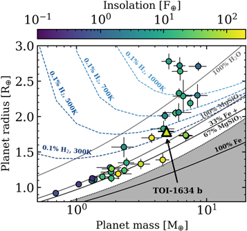
Figure 8. Mass–radius diagram for small planets transiting M dwarfs and with precisely measured masses of  . TOI-1634 b is depicted by the lone triangle marker. The solid curves are illustrative interior structure models of 100% water, 100% magnesium silicate rock, 33% iron plus 67% rock (i.e., Earth-like), and 100% iron (Zeng & Sasselov 2013). The dashed curves depict models of enveloped terrestrials consisting of an Earth-like core enveloped in H2 gas with a 1% envelope mass fraction over a range of equilibrium temperatures. The dashed curve bounds the forbidden shaded region according to models of maximum collisional mantle stripping by giant impacts (Marcus et al. 2010).
Download figure:
Standard image High-resolution imageAlternatively, the fact that TOI-1634 b appears to be underdense relative to an Earth-like composition may be explained by a rocky composition that is enhanced in Ca- and Al-rich minerals rather than the typical Earth-like rocky compounds of magnesium silicates and iron (Dorn et al. 2019). At temperatures exceeding 1200 K within the midplane of the protoplanetary disk, the condensation fraction of Ca and Al is greater than that of Mg, Si, and Fe, which would provide more solid Ca- and Al-rich material from which rocky planets could form. As such, if TOI-1634 b formed in situ, it could belong to an alternative class of super-Earths whose rocky interior compositions differ significantly from the Earth and the majority of super-Earths.
Among the M-dwarf planets depicted in Figure 8 that are underdense relative to an Earth-like composition (denoted sub-Neptunes for simplicity), all of which are larger than 1.7 R⊕, TOI-1634 b is fairly unique in that the insolation it receives is uncharacteristically high. With an insolation flux of  , TOI-1634 b is the second most highly irradiated sub-Neptune orbiting an M dwarf (TOI-1685 b receives an insolation flux of
  Bluhm et al. 2021). This fact makes TOI-1634 b a somewhat uniquely accessible sub-Neptune for atmospheric characterization. The physical implications of a high equilibrium temperature on a sub-Neptune will have to wait for such observations (see Section 5.3). Other examples of well-studied USP sub-Neptunes around FGK stars include 55 Cnc e (Bourrier et al. 2018) and WASP-47 e (Vanderburg et al. 2017). The exact cause of these peculiar underdense planets is unknown but it has been noted that 55 Cnc and WASP-47 are the most metal-rich stars among small USP planet hosts ([Fe/H]
 dex, [Fe/H]
 dex; Dai et al. 2019), and they are the only known systems to contain both a small USP planet and a close-in giant planet, the presence of which can influence icy pebble drift and thus the water inventory of the inner disk (Bitsch et al. 2021). For comparison, TOI-1634 also appears to be somewhat metal-rich (
![$[\mathrm{Fe}/{\rm{H}}]={0.23}_{-0.08}^{+0.07}$](https://content.cld.iop.org/journals/1538-3881/162/2/79/revision1/ajac0157ieqn228.gif) dex) but our RV analysis does not provide any evidence for an outer giant planet. Further investigations of these features, and the possibility that these USP planets are representative of a new class of Ca- and Al-rich super-Earths, may provide clues of possible evolutionary pathways that are able to produce sub-Neptune USP planets.
dex) but our RV analysis does not provide any evidence for an outer giant planet. Further investigations of these features, and the possibility that these USP planets are representative of a new class of Ca- and Al-rich super-Earths, may provide clues of possible evolutionary pathways that are able to produce sub-Neptune USP planets.
5.2. Implications for the Emergence of the Radius Valley around Early M Dwarfs
A variety of physical mechanisms have been proposed to explain the emergence of the radius valley. These include models of thermally driven atmospheric mass loss such as photoevaporation: hydrodynamic escape driven by stellar XUV heating (Owen & Wu 2013; Jin et al. 2014; Lopez & Fortney 2014; Chen & Rogers 2016; Owen & Wu 2017; Jin & Mordasini 2018; Lopez & Rice 2018), and core-powered mass loss: atmospheric heating and escape driven by the planet’s own cooling luminosity (Ginzburg et al. 2018; Gupta & Schlichting 2019, 2020). Conversely, the radius valley has also been proposed as a natural outcome of the formation of rocky Super-Earths and enveloped terrestrials from a gas-poor (but not gas-depleted) environment, without the need to invoke any subsequent atmospheric escape (Lee & Connors 2021). When parameterizing the slope of the radius valley via  , each of the photoevaporation, core-powered mass loss, and gas-poor formation models predict that
 ![$\beta \in [-0.15,-0.09]$](https://content.cld.iop.org/journals/1538-3881/162/2/79/revision1/ajac0157ieqn230.gif) (Lopez & Rice 2018; Gupta & Schlichting 2020; Lee & Connors 2021). Whereas if enveloped terrestrials form within the first few Myr when the gaseous disk was still present, and terrestrial planet formation proceeds at late times after the dissipation of the gaseous disk in a gas-depleted environment, then the period dependence of the radius valley is expected to exhibit the opposite sign (
(Lopez & Rice 2018; Gupta & Schlichting 2020; Lee & Connors 2021). Whereas if enveloped terrestrials form within the first few Myr when the gaseous disk was still present, and terrestrial planet formation proceeds at late times after the dissipation of the gaseous disk in a gas-depleted environment, then the period dependence of the radius valley is expected to exhibit the opposite sign ( Lopez & Rice 2018).
The radius valley around Sun-like stars with  K has been well characterized with both Kepler and K2 (e.g., Fulton et al. 2017; Fulton & Petigura 2018; Van Eylen et al. 2018; Martinez et al. 2019; Zink et al. 2020) and measurements of β take on values
 ![$\in [-0.11,-0.09]$](https://content.cld.iop.org/journals/1538-3881/162/2/79/revision1/ajac0157ieqn233.gif) (Van Eylen et al. 2018; Martinez et al. 2019). Thus, a thermally driven mass-loss or gas-poor formation model is favored in this stellar-mass regime. However, around lower-mass mid-K to mid-M dwarfs, there is tentative evidence that β flattens and becomes consistent with predictions from gas-depleted formation (
(Van Eylen et al. 2018; Martinez et al. 2019). Thus, a thermally driven mass-loss or gas-poor formation model is favored in this stellar-mass regime. However, around lower-mass mid-K to mid-M dwarfs, there is tentative evidence that β flattens and becomes consistent with predictions from gas-depleted formation ( Cloutier & Menou 2020). This suggests that gas-depleted formation, similar to the suspected formation of the inner solar system, might begin to dominate the close-in planet population around M dwarfs. The distinct slopes of the radius valley’s period dependence naturally carve out a region of the orbital period–planet radius parameter space within which the models make opposing predictions as to whether any planets located therein should have a rocky Earth-like composition or instead be enveloped in H/He gas (Figure 9). We refer to these radius valley planets around M dwarfs as keystone planets as they can be used to directly rule out certain models from precise mass and radius measurements. We note however that not all keystone planets are equally useful for constraining model applicability as, for example, keystone planets with orbital periods between 10 and 40 days can be consistent with both models given typical uncertainties on their planetary radii.
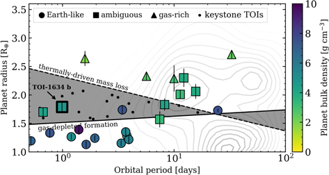
Figure 9. Period–radius diagram for small planets transiting M dwarfs and with precisely measured RV masses of  . The gray contours depict the planetary occurrence rates around low-mass stars from Kepler and K2 (Cloutier & Menou 2020). The dashed and solid lines depict model predictions of the location of the M-dwarf radius valley from thermally driven mass loss and from gas-depleted formation, respectively. The intermediate shaded regions host the so-called keystone planets like the newly discovered TOI-1634 b. The marker shapes depict planets whose bulk compositions have been determined to be Earth-like (circles), gas-rich (triangles), or ambiguous (see text for possible explanations; squares). The color bar highlights each planet’s bulk density. The dots depict keystone TOIs that have yet to be vetted as validated planets or false positives.
Download figure:
Standard image High-resolution imageWith its orbital period of 0.989 days and its size of  R⊕, TOI-1634 b sits inside of the M-dwarf radius valley between the model predicted slopes (Figure 9). Figure 9 also features the subset of M-dwarf planets from Figure 8 with precise RV masses. Planets are classified based on their bulk compositions inferred from their masses and radii. Earth-like planets are defined as those consistent with an Earth-like compositional curve, gas-rich planets cannot be explained by even 100% water composition and require an extended H/He envelope, and the intermediate planets we broadly classify as “ambiguous” given that they may be explained by a variety of compositions including a H/He envelope, a volatile-rich composition, or a rocky composition that is enhanced in Ca and Al. Our analysis revealed that TOI-1634 b is inconsistent with an Earth-like composition at
  50
and requires an alternative physical interpretation to explain its mass and radius. As such, we assign TOI-1634 b to the “ambiguous” category.
50
and requires an alternative physical interpretation to explain its mass and radius. As such, we assign TOI-1634 b to the “ambiguous” category.
Regardless of the true composition of TOI-1634 b, the inconsistency of TOI-1634 b’s mass and radius with an Earth-like composition indicates that it is not compatible with models of thermally driven mass loss of Earth-like cores and may support the gas-depleted formation model. However, this picture may not be so clear because models of thermally driven mass loss have focused on rocky planets that have Earth-like compositions (e.g., Owen & Wu 2017; Gupta & Schlichting 2019) and have not considered the possibility of other types of rocky planets that are Ca- and Al-enriched. But if the gas-depleted formation scenario was operating in the TOI-1634 system then TOI-1634 b would have formed early on within the gaseous disk’s lifetime and subsequently accreted a primordial H/He envelope that was not entirely lost to space. However, this presents a clear ambiguity in that if TOI-1634 b had accumulated a primordial H/He envelope at its current location, then such an envelope should have been rapidly lost to thermal escape. The curious case of TOI-1634 b may be reconciled if it migrated inward to its current location after the extended XUV active phase (0.5–1 Gyr; Shkolnik & Barman 2014; France et al. 2016) and due to its hosting of a high mean molecular weight atmosphere. Alternatively, TOI-1634 b may indeed be a rocky planet that is enhanced in Ca and Al and hence is underdense relative to an Earth-like rocky planet (Dorn et al. 2019). However, each of these scenarios is speculative as they are presently indistinguishable with the data available.
The compositions of the keystone planets classified as “ambiguous” make it difficult to robustly establish gas-depleted formation as the mechanism responsible. If we wish to establish the importance of the gas-depleted formation scenario around M dwarfs, we recommend that RV follow-up campaigns of transiting planets focus on small, potentially rocky planets with orbital periods ≳20 days (e.g., the super-Earth LHS 1140 b with P = 24.7 days; Dittmann et al. 2017). The thermally driven hydrodynamic escape timescales for such planets are typically longer than the age of the system such that if they turn out to be rocky, such compositions cannot be explained by atmospheric mass loss and those planets are likely to have formed rocky. TESS has already revealed five such planet candidates 51 that we recommend be targeted for detailed follow-up.
The fact still remains that the composition of TOI-1634 b does not resemble an Earth-like composition at  , a result that supports the notion that thermally driven mass loss may not dominate the sculpting of the close-in planet population around M dwarfs with masses less than or similar to TOI-1634 (≲0.5 M⊙). This proposition is further supported by the composition of the other keystone USP planet in Figure 9: the sub-Neptune TOI-1685 b whose host stellar mass is nearly identical to that of TOI-1634 (
 M⊙; Bluhm et al. 2021). However, because models of thermally driven mass loss have assumed that the underlying cores of the close-in planet population are Earth-like, if TOI-1634 b is rocky but not Earth-like (i.e., Ca- and Al-enriched), then its mass and radius may still be consistent with models of thermally driven mass loss.
5.3. Prospects for Atmospheric Characterization
The mass and radius of TOI-1634 b strongly suggest the presence of a gaseous envelope, which may be accessible with JWST. Given the unusual combination of TOI-1634 b’s location in mass–radius space and its close orbital separation, TOI-1634 b occupies a unique region of the parameter space wherein it would be particularly interesting to distinguish between different atmospheric compositions. For example, a H2O-rich atmosphere would likely be indicative of a substantial initial water reservoir (Schaefer et al. 2016; Kite & Barnett 2020) whereas a CO2-rich atmosphere may be produced by a runaway greenhouse if a significant portion of the planet’s water inventory was photolyzed and lost to space. Given its USP, TOI-1634 b is an attractive candidate to distinguish between these atmosphere models via thermal emission observations as atmospheric signatures are likely to be more easily accessible than in transmission (Morley et al. 2017b). Emission versus transmission spectroscopy is also less susceptible to signal attenuation by either clouds/hazes or high mean molecular atmospheres (Miller-Ricci et al. 2009), and it can also be used to probe the atmospheric temperature profile.
Assuming a day-side temperature of  K, the analytical emission spectroscopy metric (ESM; Kempton et al. 2018) for TOI-1634 is approximately 23. This value illustrates TOI-1634 b’s favorability for emission spectroscopy observations when compared to the ESM values of the flagship M-dwarf planets LHS 3844 b (Vanderspek et al. 2019), GJ 1132 b (Berta-Thompson et al. 2015), and TRAPPIST-1 b (Gillon et al. 2017), whose ESM values are 30, 10, and 4, respectively. However, we note that unlike TOI-1634 b, each of these planets is consistent with a rocky bulk composition. Malik et al. (2019) calculated the number of eclipse observations needed to distinguish between either of the aforementioned atmospheric scenarios and a clear solar-composition atmosphere for the flagship M-dwarf planets LHS 3844 b, GJ 1132 b, and TRAPPIST-1 b. By scaling the Malik et al. (2019) results for GJ 1132 b to the expected emission S/N of TOI-1634 b, we estimate that the H2O- and CO2-rich atmospheres could be distinguishable for one another with two to four JWST/MIRI eclipses in its slitless LRS mode. Similarly, we expect five eclipses are required in order to distinguish between the H2O and solar-composition models using NIRSpec/G395M.
For the sake of completeness, we also estimate the number of transit observations needed to detect transmission features. Assuming an isothermal temperature profile at the zero-albedo equilibrium temperature  K, the expected depths of transmission features at two scale heights (Stevenson 2016; Fu et al. 2017) in a solar-composition, H2O-dominated, or CO2-dominated atmosphere are 102, 13, and 5 ppm, respectively. We simulate NIRISS/SOSS (0.8–2.8 μm) and NIRSpec/G395M (2.8–5.2 μm) observations using PandExo (Batalha et al. 2017) and find that only features in a clear solar-composition atmosphere would be detectable at
  with fewer than 10 transits. However, a clear H/He-dominated atmosphere for TOI-1634 b is highly unlikely given that such an atmosphere is unstable at 121 times Earth’s insolation flux (Lopez 2017). High-altitude clouds would also be increasingly detrimental to feature detection in transmission, whereas the presence of clouds may be more easily inferred with secondary eclipse observations as a high day-side albedo would distinguish clouds from a bare rocky surface with fewer than 10 visits (Mansfield et al. 2019).
5.4. Constraints on Additional Planets
5.4.1. RV Sensitivity
M dwarfs hosting multiplanet systems are ubiquitous. Focusing on Kepler stars with  K and log g > 3, Dressing & Charbonneau (2015) found that late K- to early M-dwarf stars host 2.5 ± 0.2 planets smaller than 4 R⊕ and out to 200 days per star. Similarly, Gaidos et al. (2016) confirmed these results over a similar range of planetary radii (1–4 R⊕) and orbital periods (1.5–180 days): 2.2 ± 0.3 planets per early M dwarf. Complimentary studies of M-dwarf planet occurrence rates from RV studies have yielded similar results to those obtained from the Kepler transit survey (Bonfils et al. 2013; Tuomi et al. 2014). Although largely limited by poor counting statistics from the Kepler mission, preliminary occurrence rate calculations around mid-M dwarfs from Muirhead et al. (2015) and Hardegree-Ullman et al. (2019) have posited that compact systems (
 days) of multiple planets are common and perhaps increasingly so as the host stars become less massive. Indeed, there have been a number of apparently single transiting M-dwarf systems, which later revealed additional planets following one or both of photometric and RV follow-up (e.g., GJ 357 c, d; Luque et al. 2019, GJ 1132c; Bonfils et al. 2018, GJ 3473c; Kemmer et al. 2020, K2-18c; Cloutier et al. 2019b, LHS 1140c; Ment et al. 2019).
With the existence of one known planet orbiting TOI-1634, it is reasonable to think that a second planet may exist but as yet remains undetected because of its small size, long orbital period, or because its orbit is not in a transiting configuration. Here we place limits on hypothetical planets around TOI-1634 given our RV time series. Specifically, we compute the RV sensitivity to planets around TOI-1634 as a function of planet mass and orbital period via a set of injection-recovery tests. We run a Monte Carlo simulation of 104 realizations by injecting synthetic Keplerian signals into the residuals of the HARPS-N RV time series after the removal of the MAP solution for TOI-1634 b. In each realization, we simulate a single planet. Planet masses and orbital periods are sampled uniformly in log space with the following bounds: 0.1–20 M⊕ and 1–200 days. Orbital phases are sampled uniformly from  . We sample the orbital inclination from the Gaussian distribution
  , where
  and the dispersion in mutual inclinations of
  follows from studies of multiplanet M-dwarf systems (Ballard & Johnson 2016). The stellar mass is also sampled from its posterior and is used to calculate the corresponding RV semiamplitude assuming a circular orbit. We then inject the synthetic Keplerian signal into the RV residuals, thus preserving any residual noise from systematics or uncorrected stellar activity. The individual measurement uncertainties and timestamps are left unchanged.
We attempt to recover injected planets following a two-step process. The search for nontransiting planets in RV time series does not have the benefit of a priori knowledge of the planet’s period and phase. Instead, probable signals must show a prominent periodic signal in the GLS periodogram with a FAP  %.
52
Second, the six-parameter Keplerian model must be strongly favored over the null hypothesis (i.e., a flat line). For the purpose of model comparison, we adopt the Bayesian information criterion
%.
52
Second, the six-parameter Keplerian model must be strongly favored over the null hypothesis (i.e., a flat line). For the purpose of model comparison, we adopt the Bayesian information criterion  , where
  is the likelihood of the RV data given the assumed model, ν is the number of model parameters, and N = 32 is the number of RV measurements. Taken together, we claim the successful recovery of an injected planet if and only if the GLS periodogram power of the largest periodic signal within 10% of the injected period has FAP
  % and the BIC value of the Keplerian model is greater than 10 times the BIC of the null hypothesis. The sensitivity of our RV data set is defined as the ratio of a number of recovered planets over the number of injected planets and is depicted in Figure 10.
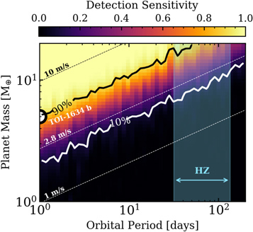
Figure 10. RV detection sensitivity to planets orbiting TOI-1634 as a function of planet mass and orbital period. The solid line contours highlight the 10% and 90% sensitivity levels. The thin dashed lines represent lines of constant semiamplitude with illustrative values equal to 1 m s−1, the median dispersion in our HARPS-N time series (2.8 m s−1), and 10 m s−1. The circle marker highlights TOI-1634 b. The vertical shaded region spans the habitable zone of TOI-1634 whose inner and outer edges are defined by the recent Venus and early Mars boundaries (Kopparapu et al. 2013).
Download figure:
Standard image High-resolution imageUnsurprisingly, we find that the mass and orbital period of TOI-1634 b lie within the region where our RV sensitivity is high (i.e., 90%). Figure 10 also reveals that at an orbital period of 1 day, we are sensitive to approximately 50% of planets at 3 M⊕ and to all planets ≳5 M⊕. Within 10 days, we are sensitive to all planets  M⊕. Our sensitivity to the majority of terrestrial planets (
 M⊕) at orbital periods >3 days is relatively poor due to the large RV dispersion and the modest number of measurements (N = 32). If we adopt the empirical recent Venus and early Mars habitable zone (HZ) limits from Kopparapu et al. (2013; i.e., 30–125 days), we find that we are only sensitive to very massive HZ planets (>15 M⊕). Unfortunately, any such planet would be an improbable candidate for habitable conditions given that the most massive M-dwarf planets with Earth-like bulk compositions are less massive than 7–8 M⊕ (
 M⊕; Ment et al. 2019,
  M⊕; Cloutier et al. 2020b) such that any planet whose mass exceeds 15 M⊕ would have to host a massive H/He envelope, thus rendering its surface uninhabitable.
5.4.2. Search for Transit Timing Variations
We also conduct a search for transit timing variations (TTVs) by fitting the individual TESS transits in the detrended PDCSAP light curve and the select high-S/N seeing-limited transits from Figure A2. We apply a transit model with all model parameters fixed other than the time of midtransit. We fit the 20 TESS and 11 seeing-limited transits separately and achieve typical photometric precisions on the individual transit times of 4.4 and 7.5 minutes, respectively. We find that the deviation of the individual transit times from a linear ephemeris is consistent with a flat line and shows a low rms of approximately 30 s in the TESS transits, which are of comparatively higher quality. We conclude that TOI-1634 b shows no evidence for TTVs.
5.5. An Independent Analysis of the TOI-1634 System
Through the international TFOP collaboration, multiple RV teams began independent follow-up campaigns to characterize the mass of the planet candidate TOI-1634.01. Our work based on HARPS-N data presented herein represents one such effort but we acknowledge a second RV analysis of this system, which was conducted independently of our own (Hirano et al. 2021). The submissions of these works were coordinated between the two groups but their respective data, analyses, and manuscripts were kept intentionally separate.
Hirano et al. (2021) presented the mass characterization of two USP planets, including TOI-1634 b, using infrared RV measurements taken with the IRD spectrograph at Subaru (Tamura et al. 2012). Their resulting RV semiamplitude is discrepant from ours at 5σ as they measure a larger RV semiamplitude of  m s−1 and show that TOI-1634 b is likely consistent with an Earth-like composition. Similarly, the second USP planet presented in Hirano et al. (2021; TOI-1685 b) was also found to be consistent with an Earth-like composition, whereas this planet was previously shown to be underdense relative to an Earth-like composition using CARMENES RV measurements (Bluhm et al. 2021). The similar analyses conducted in this work, in Hirano et al. (2021), and in Bluhm et al. (2021) suggest that the differences in the IRD results compared to HARPS-N for TOI-1634 b and compared to CARMENES for TOI-1685 b are derived from the IRD data and not from issues with any one group’s analysis. The exact cause of these discrepancies is currently unknown, and their resolution is left as a future exercise.
6. Summary and Conclusions
We presented the discovery of TOI-1634 b, a USP keystone planet orbiting an M2 dwarf, which sits within a radius valley. Keystone planets are useful because knowledge of their bulk composition may be used to distinguish between radius valley emergence models of thermally driven mass loss and gas-depleted formation. Our work has produced the following main findings:
- 1.TOI-1634 b is a sub-Neptune USP planet with
 days,
R⊕, and
M⊕. The mass and radius of TOI-1634 b are inconsistent with an Earth-like composition at .
days,
R⊕, and
M⊕. The mass and radius of TOI-1634 b are inconsistent with an Earth-like composition at . - 2.The composition of TOI-1634 b deviates from expectations from the close-in planet population and may be explained by either a volatile-rich layer with a high mean molecular weight atmosphere that is resistant to atmospheric loss or by a rocky composition that is Ca- and Al-enriched and consequently underdense relative to Earth.
- 3.The bulk composition of TOI-1634 b is inconsistent with models of thermally driven mass loss (i.e., photoevaporation and core-powered mass loss) and with gas-poor formation. Instead, TOI-1634 b appears to support the gas-depleted formation model and would suggest that this formation mechanism may start to dominate the close-in planet population around M dwarfs with masses
M⊙ if indeed TOI-1634 b is not rocky.
- 4.Emission spectroscopy observations will help to establish the chemical and physical properties that make the atmosphere of TOI-1634 b resistant to hydrodynamic escape. Atmospheric models of solar-composition, H2O-dominated, and CO2-dominated may be distinguished with two to five eclipse observations with JWST/MIRI or JWST/NIRSpec.
- 5.Upon evaluating our RV sensitivity to additional planets, we are able to rule out terrestrial-mass planets more massive than 5 M⊕ within 2–3 days and planets >15 M⊕ within the star’s habitable zone between 30 and 125 days.


The inconsistency of the mass and radius of TOI-1634 b with an Earth-like composition suggests that the gas-depleted formation scenario is favored over thermally driven mass loss to explain its mass and radius. However, the unknown underlying composition of TOI-1634 b makes this statement nonrobust. To determine the applicability of gas-depleted formation around M dwarfs, we advocate for the mass characterization of small planets with periods ≳20 days. If these planets are determined to be predominantly rocky, that would support the gas-depleted formation interpretation because the mass-loss timescales for these planets are too long for thermally driven mass loss to explain their rocky compositions.
R.C. is supported by a grant from the National Aeronautics and Space Administration in support of the TESS science mission.
C.D.D. acknowledges support from the Hellman Fellows Fund, the Alfred P. Sloan Foundation, the David & Lucile Packard Foundation, and the NASA Exoplanets Research Program (XRP) through grant 80NSSC20K0250.
This work is made possible by a grant from the John Templeton Foundation. The opinions expressed in this publication are those of the authors and do not necessarily reflect the views of the John Templeton Foundation. This material is based on work supported by the National Aeronautics and Space Administration under grant No. 80NSSC18K0476 issued through the XRP Program.
The financial support from the agreement ASI-INAF n.2018-16-HH.0 is gratefully acknowledged.
Based on observations made with the Italian Telescopio Nazionale Galileo (TNG) operated by the Fundación Galileo Galilei (FGG) of the Istituto Nazionale di Astrofisica (INAF) at the Observatorio del Roque de los Muchachos (La Palma, Canary Islands, Spain).
The HARPS-N project has been funded by the Prodex Program of the Swiss Space Office (SSO), the Harvard University Origins of Life Initiative (HUOLI), the Scottish Universities Physics Alliance (SUPA), the University of Geneva, the Smithsonian Astrophysical Observatory (SAO), the Italian National Astrophysical Institute (INAF), the University of St Andrews, Queens University Belfast, and the University of Edinburgh.
This work has made use of data from the European Space Agency (ESA) mission Gaia (https://www.cosmos.esa.int/gaia), processed by the Gaia Data Processing and Analysis Consortium (DPAC, https://www.cosmos.esa.int/web/gaia/dpac/consortium). Funding for the DPAC has been provided by national institutions, in particular the institutions participating in the Gaia Multilateral Agreement.
This work makes use of observations from the LCOGT network. Part of the LCOGT telescope time was granted by NOIRLab through the Mid-Scale Innovations Program (MSIP). MSIP is funded by NSF.
This article is based on observations made with the MuSCAT2 instrument, developed by ABC, at Telescopio Carlos Sánchez operated on the island of Tenerife by the IAC in the Spanish Observatorio del Teide.
This work is partly supported by JSPS KAKENHI grant numbers JP18H01265 and JP18H05439, and JST PRESTO grant No. JPMJPR1775, and a University Research Support Grant from the National Astronomical Observatory of Japan (NAOJ).
Resources supporting this work were provided by the NASA High-End Computing (HEC) Program through the NASA Advanced Supercomputing (NAS) Division at Ames Research Center for the production of the SPOC data products.
Some of the Observations in the paper made use of the High-Resolution Imaging instrument ’Alopeke. ’Alopeke was funded by the NASA Exoplanet Exploration Program and built at the NASA Ames Research Center by Steve B. Howell, Nic Scott, Elliott P. Horch, and Emmett Quigley. ’Alopeke was mounted on the Gemini North telescope of the international Gemini Observatory, a program of NSF’s OIR Lab, which is managed by the Association of Universities for Research in Astronomy (AURA) under a cooperative agreement with the National Science Foundation on behalf of the Gemini partnership: the National Science Foundation (United States), National Research Council (Canada), Agencia Nacional de Investigación y Desarrollo (Chile), Ministerio de Ciencia, Tecnología e Innovación (Argentina), Ministério da Ciência, Tecnologia, Inovações e Comunicações (Brazil), and Korea Astronomy and Space Science Institute (Republic of Korea).
Facilities: TESS - , ASAS-SN - , TRES - , LCOGT - , MuSCAT2 - , OAA - , RCO - , Gemini/’Alopeke - , Lick/ShARCS - , TNG/HARPS-N. -
Software: AstroImageJ (Collins et al. 2017), astropy (Astropy Collaboration et al. 2013, 2018), BANZAI (McCully et al. 2018), batman (Kreidberg 2015), BGLS (Mortier et al. 2015), celerite (Foreman-Mackey et al. 2017), emcee (Foreman-Mackey et al. 2013), exoplanet (Foreman-Mackey et al. 2019), PandExo (Batalha et al. 2017), PyMC3 (Salvatier et al. 2016), scipy (Virtanen et al. 2020), STARRY (Luger et al. 2019), Tapir (Jensen 2013), TERRA (Anglada-Escudé & Butler 2012).
Appendix: Additional Planet Validation Figures
Here we display our follow-up observations of TOI-1634. Figure A1 depicts our reconnaissance spectroscopy, Figure A2 depicts our seeing-limited transit observations, and Figure A3 depicts our high-resolution imaging observations.
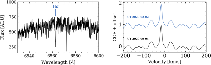
Figure A1. Key takeaways from TRES reconnaissance spectroscopy of TOI-1634. Left panel:  in absorption indicating a chromospherically inactive star. Right panel: the CCF of each TRES epoch reveals a single-lined spectrum with no resolved rotational broadening (i.e.,
  < 3.4 m s−1).
Download figure:
Standard image High-resolution image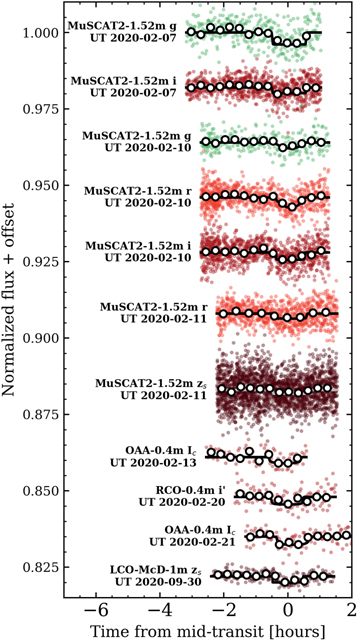
Figure A2. Select seeing-limited photometric light curves of TOI-1634 b transit events with particularly low-S/N light curves omitted. The light curves are vertically offset for clarity. Annotated next to each light curve are the observing facility, the passband, and the UT observation date.
Download figure:
Standard image High-resolution image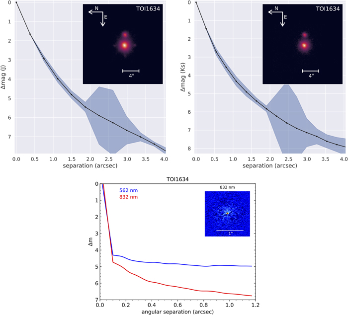
Figure A3. High-resolution imaging observations of TOI-1634. First and second panels: the J- (left) and KS
-band (right) contrast curves and rms errors from ShARCS AO-imaging. The inset in each panel shows the band’s stacked image. Third panel: 5σ contrast curves from ’Alopeke speckle imaging at 562 nm and 832 nm along with the reconstructed 832 nm image in the inset. Other than the known companion located  west of TOI-1634, no additional companions or background sources are revealed by our high-resolution imaging.
Download figure:
Standard image High-resolution imageFootnotes
- 44
RUWE = 1.23, where RUWE = 1 is assigned to well-behaved single star solutions and RUWE > 1.4 likely indicates a nonsingle star.
- 45
Based on the TESS Web Viewing Tool (https://heasarc.gsfc.nasa.gov/cgi-bin/tess/webtess/wtv.py).
- 46
“Probing the Landscape of Cool Dwarf Planet Occurrence.” PI: Dressing.
- 47
https://archive.stsci.edu/missions/tess/doc/tess_drn/tess_sector_27_drn38_v02.pdf. The sky background algorithm was updated to mitigate the background bias starting with Sector 27.
- 48
- 49
Due to the high probability of TOI-1634 b being tidally circularized, we also tested a model with a fixed circular orbit and found that the resulting RV semiamplitude and its measurement precision are effectively insensitive to the assumption of a circular orbit.
- 50
Similarly, the mass of TOI-1634 b is inconsistent with a 100% MgSiO3 composition at
. - 51
TOIs 198.01, 203.01, 256.01, 1266.02, 2094.01, and 2095.02.
- 52
However, we note that this need not be the case for massive outer companions, which can induce detectable long-term trends without a prominent signal in the GLS at its orbital frequency.
