Abstract
Stellar kinematics is a powerful tool for understanding the formation process of stellar associations. Here, we present a kinematic study of the young stellar population in the Rosette nebula using recent Gaia data and high-resolution spectra. We first isolate member candidates using the published mid-infrared photometric data and the list of X-ray sources. A total of 403 stars with similar parallaxes and proper motions are finally selected as members. The spatial distribution of the members shows that this star-forming region is highly substructured. The young open cluster NGC 2244 in the center of the nebula has a pattern of radial expansion and rotation. We discuss its implication on the cluster formation, e.g., monolithic cold collapse or hierarchical assembly. On the other hand, we also investigate three groups located around the border of the H ii bubble. The western group seems to be spatially correlated with the adjacent gas structure, but their kinematics is not associated with that of the gas. The southern group does not show any systematic motion relative to NGC 2244. These two groups might be spontaneously formed in filaments of a turbulent cloud. The eastern group is spatially and kinematically associated with the gas pillar receding away from NGC 2244. This group might be formed by feedback from massive stars in NGC 2244. Our results suggest that the stellar population in the Rosette Nebula may form through three different processes: the expansion of stellar clusters, hierarchical star formation in turbulent clouds, and feedback-driven star formation.
1. Introduction
Star formation hierarchically takes place on various spatial scales (Elmegreen et al. 2000; Gouliermis 2018). Stellar complexes are the largest components of galactic superstructures spanning hundreds of parsecs. These complexes are composed of several stellar associations that extend up to several tens of parsecs. Single or multiple stellar clusters (a few parsecs) and a distributed stellar population constitute these stellar associations (Blaauw 1964; Koenig et al. 2012). The formation of these components is thought to be physically interconnected in space and time. In this context, stellar associations would be basic units of star formation in galaxies. Indeed, the majority of stars tend to form in such stellar systems (Lada & Lada 2003; Porras et al. 2003), and their initial mass functions are very similar to that derived from field stars in the Galaxy (Miller & Scalo 1978; Briceño et al. 2007).
Stellar associations are gravitationally unbound and substructured (Mel’nik & Dambis 2017; Kuhn et al. 2019; Lim et al. 2019, 2020). The internal structure and kinematics are the keys to understanding their formation process. A classical model attempted to explain the observed structures and unboundedness of OB associations in the context of dynamical evolution of embedded clusters. Once embedded clusters have formed in giant molecular clouds, they begin to expand after rapid gas expulsion by winds and outflows of embedded OB stars (Tutukov 1978; Hills 1980; Lada et al. 1984; Kroupa et al. 2001; Banerjee & Kroupa 2013, 2015). Kroupa et al. (2001) performed N-body simulations for model clusters with the properties similar to those of the Orion Nebula Cluster that were observationally constrained. As a result, they found that only about 30% of the initial cluster members remain in the model clusters. Their results imply that open clusters can be the cores of unbound OB associations.
The structural features observed in star-forming complexes are similar to those found in molecular clouds (Dickman et al. 1990; Elmegreen et al. 2000; André 2015). It has been suggested that turbulence is responsible for the origin of these substructures in molecular clouds (Larson 1981; Padoan et al. 2001). Density fluctuation caused by turbulence results in locally different star formation efficiency, and therefore groups of stars with different stellar densities form along the substructures on short timescales (Bonnell et al. 2011; Kruijssen 2012).
On the other hand, massive stars can play crucial roles in regulating star formation in either constructive or destructive way. Far-ultraviolet radiation and stellar wind from massive stars disperse the remaining gas in their close neighborhood, lowering star formation efficiency and eventually terminating star formation (Dale et al. 2012, 2013). In contrast, expanding H ii bubbles driven by massive stars can compress the surrounding material, triggering the formation of new generations of stars further away from the massive stars (Elmegreen & Lada 1977). OB associations could also form through this self-propagating star formation.
Explaining the formation of stellar associations from observed features via one specific model seems complicated and impossible. The signature of dynamical evolution of central stellar clusters has been reported. For example, a pattern of expansion has been detected in young stellar clusters within many associations (Kounkel et al. 2018; Cantat-Gaudin et al. 2019; Kuhn et al. 2019; Lim et al. 2019). Recently, a kinematic study showed that a distributed stellar population spread over 20 pc in W4 can be formed by cluster members radially escaping from the central cluster IC 1805 (Lim et al. 2020). In addition, even larger-scale expansion of associations spanning several hundreds of parsecs toward the Perseus arm was also reported (Román-Zúñiga et al. 2019; Dalessandro et al. 2021).
Several stellar groups were found at the border of the W4 H ii region (Panwar et al. 2019), and their projected distance from IC 1805 cannot be explained by crossing time of the escaping stars (Lim et al. 2020). Instead, feedback-driven star formation may be a possible explanation for the formation of these groups. Many signposts of feedback-driven star formation have been steadily reported in various star-forming regions (SFRs; Fukuda et al. 2002; Sicilia-Aguilar et al. 2004; Koenig et al. 2008, etc.). For instance, a stellar group in NGC 1893 is located in the vicinity of the gas pillar Sim 130 (Marco & Negueruela 2002; Sharma et al. 2007). This group is younger than the central cluster containing massive O-type stars (Lim et al. 2014) and receding away from the cluster at a velocity similar to that of the gas pillar (Lim et al. 2018).
The signatures of hierarchical star formation in turbulent clouds have been investigated using stellar proper motions (PMs) under the assumption that the age of OB associations is young enough to preserve the kinematic properties of their natal clouds just before onset of star formation. For example, the Cygnus OB2 and Carina OB1 associations are composed of spatially and kinematically distinct subgroups (Lim et al. 2019). In addition, a correlation between the size and two-dimensional velocity dispersion of these subgroups was found, which has a power-law index similar to that found in molecular clouds (Larson 1981). These first observational results were supported by an extensive kinematic study on larger samples of the Galactic OB associations (Ward et al. 2020).
Hence, we hypothesize that stellar associations may form through three different processes, i.e., dynamical evolution of stellar clusters, feedback from massive stars, and star formation in turbulent clouds. In this context, the Rosette Nebula, the most active SFR in the Monoceros OB2 association, is an ideal site to examine the hypothesis because this region is composed of several stellar groups in a range of 30 pc. The open cluster NGC 2244 is centered at the cavity of the Rosette Nebula and contains several tens of OB stars (Román-Zúñiga & Lada 2008; Mahy et al. 2009) as well as a large number of low-mass young stellar objects (YSOs; Balog et al. 2007; Wang et al. 2008; Mužić et al. 2019). These massive stars may be the main ionizing sources of the H ii region. Additional, smaller, stellar groups are found at the border of the nebula (Li 2005; Wang et al. 2009, 2010).
The Rosette Molecular Cloud is located to the east of the H ii region, and star-forming activity is still ongoing there. Phelps & Lada (1997) reported the presence of seven embedded clusters. Later, Román-Zúñiga et al. (2008) identified four more clusters (see also the historical review on this SFR by Román-Zúñiga & Lada 2008). Extensive Spitzer and Chandra surveys continuously discovered deeply embedded clusters composed of active YSOs (Poulton et al. 2008; Wang et al. 2009; Cambrésy et al. 2013). Ybarra et al. (2013) investigated the star formation history on different scales from clusters to the molecular cloud and claimed that star formation occurred almost simultaneously across the cloud. The relation between the YSO ratio and extinction that they found suggests that the densest regions in the cloud are the favorable sites of star formation and that gas is rapidly evacuating out, lowering star formation efficiencies in the cloud.
In this study, we aim to understand the formation process of the stellar groups in the Rosette Nebula using gas and stellar kinematics. The splendid performance of the Gaia mission (Gaia Collaboration et al. 2016) opened a new window to study such young stellar systems. The Gaia astrometric data (Gaia Collaboration et al. 2021) provide a better understanding of the kinematic properties of stellar groups in this SFR when combined with spectroscopic data of stars and gas. Observations and data that we used are described in Section 2. In Section 3, the method of member selection is addressed. We investigate the motions of stars using PMs (Gaia Collaboration et al. 2021) and radial velocities (RVs) in Section 4. The physical associations between stars and gas are also probed. The formation process of NGC 2244 and stellar groups around the cluster is discussed in Section 5. Finally, we summarize our results in Section 6.
2. Data
2.1. Selection of Member Candidates
Our targets are young stars within a 1° × 1° region centered at R.A. = 06h 31m 5500, decl. = + 04°
 30
300 (J2000). This SFR (b ∼ − 2
072) is located in the Galactic plane, and therefore a large number of field interlopers are also observed in the same field of view. We intend to isolate member candidates first using multiple sets of archival data in this section, and then the final decision on membership will be made by using the recent astrometric data from the Gaia Early Data Release 3 (EDR3; Gaia Collaboration et al. 2021) in Section 3.
To identify probable member candidates in the survey region, we considered the intrinsic properties of young stars. O- and B-types stars spread over this SFR are probable member candidates because the positions of these stars are close to birthplaces within their short lifetime, particularly for O-type stars. We took a list of OB stars from the data bases of MK classifications (Mermilliod & Paunzen 2003; Reed 2003; Skiff 2009; Maíz Apellániz et al. 2013, SIMBAD) and combined them into a list after checking for duplicates. A total of 112 OB stars were selected as member candidates.
A large number of low-mass YSOs have a warm circumstellar disk. These disk-bearing YSOs appear bright in infrared passbands (Lada 1987; Gutermuth et al. 2008; Koenig et al. 2012). YSO candidates were identified using the published Spitzer and AllWISE data (Balog et al. 2007; Cutri et al. 2013); see Appendix appendix for details. We found 291 YSO candidates (10 Class I, 262 Class II, and 19 YSOs with a transitional disk) from the Spitzer data in total, while a total of 84 candidates (six Class I, 76 Class II, and two objects with a transitional disk) were identified from the AllWISE data. There are 37 YSO candidates in common between these data sets. Note that the survey region ( ) of Spitzer (Balog et al. 2007) is smaller than ours. Our list contains 338 YSO candidates in total.
We used photometric data from the Gaia Data Release 2 (DR2; Gaia Collaboration et al. 2018) instead of the recent EDR3 (Gaia Collaboration et al. 2021) because the reddening law is empirically well-established (Wang & Chen 2019) for the former. We found counterparts for all the OB stars and for 320 YSO candidates in the Gaia DR2 (Gaia Collaboration et al. 2018). In addition, we searched for counterparts of X-ray sources detected in this SFR (Wang et al. 2008, 2009, 2010). Stars found within searching radii of 10 and 1
5 were classified as X-ray sources and X-ray source candidates, respectively. A total of 720 X-ray sources and 134 candidates were found in the Gaia data. Note that the lists of X-ray sources are complete down to 0.5–1 M☉ (Wang et al. 2008, 2009, 2010).
Figure 1 displays the color–magnitude diagram (CMD) of stars in the Rosette Nebula. Most member candidates seem to occupy a specific locus in the diagram. The main-sequence turn-on is found at about 13 mag in GRP. There are several B-type stars fainter than YSOs near the main-sequence turn-on. These stars may be background early-type stars. A large fraction of the X-ray sources may be YSO candidates, while some X-ray sources appear to fall on the main-sequence band. These X-ray emitting stars may be late-type field stars. All the YSO candidates with infrared excess emission were considered as member candidates because their colors and magnitudes could vary with different levels of internal extinction by material in disks or envelopes and accretion activities (Lee et al. 2020). Photometric errors increase with brightness, and therefore we limited our sample to 840 candidates brighter than 18 mag. The selection criteria of member candidates can be summarized as below:
- 1.GRP < 18 mag.
- 2.O- or B-type stars brighter than 13.5 mag in GRP.
- 3.Class I YSOs.
- 4.Class II YSOs.
- 5.YSOs with a transitional disk.
- 6.X-ray sources within the locus (see Figure 1).
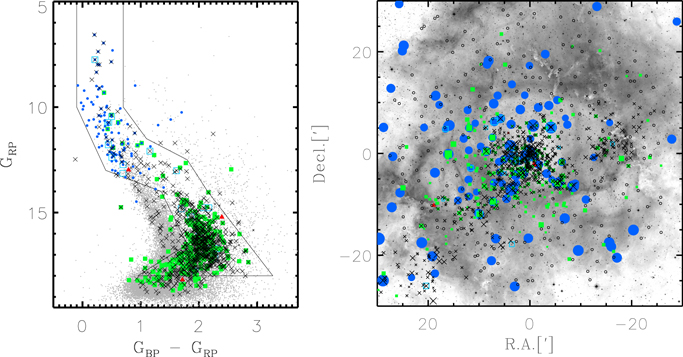
Figure 1. CMD (left) and spatial distribution (right) of member candidates in the Rosette Nebula. The photometric data were taken from Gaia Data Release 2 (Gaia Collaboration et al. 2018). Blue dots, red triangles, green filled square, cyan open square, large black crosses, small crosses, and small gray dots represent early-type star (O- or B-type), Class I, Class II, object with a transitional disk, X-ray source, X-ray source candidates, and all stars in the survey region, respectively. We set a locus (black solid line) that contains the majority of member candidates. In the right panel, the fiber positions (black open circles) are superimposed on the optical image taken from the Digitized Sky Survey. The positions of stars are relative to the coordinate R.A. = 06h 31m 5500, decl. = + 04°
 30
300 (J2000). The sizes of the symbols are proportional to the brightnesses of individual stars.
Download figure:
Standard image High-resolution image2.2. Radial Velocities
We performed spectroscopic observations of 316 YSO candidates with or without an X-ray emission and ionized gas on 2019 October 13, November 9, 13, and 18 using the high-resolution (R ∼ 34,000) multi-object spectrograph Hectochelle (Szentgyorgyi et al. 2011) on the 6.5 m telescope of the MMT observatory. The spectra of the YSO candidates were taken with the RV31 filter (5150–5300 Å) in 2 × 2 binning mode to achieve good signal-to-noise ratios. In addition, several tens of fibers were simultaneously assigned to blank sky to obtain sky spectra. The spectra of ionized gas were obtained from the fibers assigned to 238 positions on the Rosette Nebula (see Figure 1). The order separating filter OB25 (6475–6630 Å) was used to observe the forbidden line [N ii] λ6584. For calibration, dome flat and ThAr lamp spectra were also obtained just before and after the target observation. We present a summary of our observations in Table 1.
Table 1. Summary of Observations
| Date | Setup | Filter | Na | Exposure time | Binning | Seeing | |
|---|---|---|---|---|---|---|---|
| 2019 Oct 13 | 1 | RV31 | 111 | 35 minutes × 3 | 2 × 2 | 0 | |
| 2019 Nov 13 | 2 | RV31 | 110 | 40 minutes × 3 | 2 × 2 | 1 | |
| YSOs | 38 minutes × 1 | ||||||
| 3 | RV31 | 95 | 37 minutes × 1 | 2 × 2 | 1 | ||
| 35 minutes × 1 | |||||||
| 2019 Nov 18 | 3 | RV31 | 95 | 35 minutes × 2 | 2 × 2 | 1 | |
| Ionized gas | 2019 Nov 9 | 4 | OB25 | 238 | 15 minutes × 5 | 1 × 1 | 0 |
Note.
a N represents the number of observed targets.Download table as: ASCIITypeset image
We preprocessed the raw mosaic frames using the IRAF 6 /MSCRED packages in a standard way. One-dimensional spectra were then extracted from the reduced frames using the dofiber task in the IRAF/SPECRED package. Target spectra were flattened using dome flat spectra. The solutions for the wavelength calibration obtained from ThAr spectra were applied to the target and sky spectra.
Our observations were performed under bright sky condition, and therefore the scattered light was unevenly illuminated over the field of view (1° in diameter), resulting in a spatial variation of sky levels. For a given observing setup, we constructed a map of the sky levels and combined sky spectra into a master sky spectrum with an improved signal-to-noise ratio. The sky level at a target position was inferred by interpolating the position of the target to the map, and its sky spectrum was obtained from the master sky spectrum scaled to the inferred sky level. For each target spectrum, we subtracted the corresponding scaled master sky spectra and then combined sky-subtracted spectra into a single spectrum for the same target observed on the same night. Finally, the target spectra were normalized by using continuum levels traced from a cubic spline interpolation.
Since the spectra of low-mass stars contain a large number of metallic lines, their RVs can be measured more precisely than those of high-mass stars. The RVs of the YSO candidates were measured by applying a cross-correlation technique to the observed spectra. Assuming the solar chemical abundance, a total of 31 synthetic spectra in a wide temperature range of 3800–9880 K were generated from the MOOG code and Kurucz ODFNEW model stellar atmosphere (Sneden 1973; Castelli & Kurucz 2004). We derived the cross-correlation function (CCF) between the observed spectra and synthetic ones using the xcsao task in the RVSAO package (Kurtz & Mink 1998) and adopted the central velocities at the strongest CCF peaks as RVs. The errors on RVs were estimated from the equation  , where w, h, and σa
represent the full widths at half maximum of CCFs, their amplitudes, and the rms from antisymmetric components, respectively (Tonry & Davis 1979; Kurtz & Mink 1998). The measured RVs were converted to velocities in the local standard of rest frame using the IRAF/RVCORRECT task.
, where w, h, and σa
represent the full widths at half maximum of CCFs, their amplitudes, and the rms from antisymmetric components, respectively (Tonry & Davis 1979; Kurtz & Mink 1998). The measured RVs were converted to velocities in the local standard of rest frame using the IRAF/RVCORRECT task.
The spectra of 95 YSO candidates (Setup 3 in Table 1) were obtained on two different nights. The RVs of these stars were measured for each night. The median difference between two RV measurements for 52 common stars is about 0.3 km s−1, which is smaller than the mean of measurement errors (∼1.5 km s−1). The weighted means of two measurements were adopted as the RVs of given stars, where the inverse of the squared error was used as the weight value. We measured the RVs of 224 out of 316 YSO candidates in total. The spectra of the other 92 stars have insufficient signals to derive CCFs, or some of them show only emission lines.
We used the forbidden line [N ii] λ6584 to probe the kinematics of ionized gas. In general, the critical density of this line is higher than the typical electron densities of the Galactic H ii regions (Copetti et al. 2000), and photons emitted from the singly ionized nitrogen atoms are not absorbed along the line of sight. Therefore, this emission line can be used to trace the structure and kinematics of ionized gas distributed across an H ii region. The RVs of the ionized gas were measured from the line center of the best-fit Gaussian profile. We fit multiple Gaussian profiles to some complex line profiles and measured the RVs of the multiple components along the line of sight.
2.3. 12CO (J = 1−0) and 13CO (J = 1−0) Data
We used radio data to investigate the physical association between stellar groups and remaining molecular gas. The 12CO and 13CO (J = 1 − 0) line maps were obtained from Heyer et al. (2006). These radio maps covering both the Rosette Nebula and the eastern molecular cloud are useful for investigating the velocity fields of remaining molecular gas at the boundary of the H ii region. In addition, the excitation temperature Tex and column densities can be estimated by assuming of local thermodynamic equilibrium.
Since the 12CO line is, in general, optically thick, Tex can be derived from the following equation by Pineda et al. (2008):

where  is the brightness temperature at the peak intensity of 12CO. The column density of 13CO was estimated from the integrated intensity along the line of sight (in units of K km s−1) assuming an optically thin case (Pineda et al. 2008). On the other hand, the column density of 12CO was estimated using the relation of Scoville et al. (1986). However, this relation considers an optically thin case. The effects of optical depth were corrected by adopting the correction factor addressed in Schnee et al. (2007).
The integrated intensity maps of molecular gas were also constructed from the 12CO (J = 1 − 0) cube data. Note that the 12CO lines between velocities of −5 to 25 km s−1 were integrated. In addition, position–velocity diagrams were obtained by integrating the data cube along R.A. and decl.
3. Member Selection
We selected member candidates based on the intrinsic properties of young stars, but some nonmembers with similar properties may be included in our candidate list. The astrometric data from the Gaia EDR3 (Gaia Collaboration et al. 2021) allow us to better isolate genuine members. Lindegren et al. (2021) found the zero-point offset in parallax that depends on magnitude, color, and position. For reliable member selection, we corrected the zero-point offsets for the parallaxes of individual member candidates using the public Python code (Lindegren et al. 2021; https://gitlab.com/icc-ub/public/gaiadr3_zeropoint). 7
Figure 2 displays the parallax and PM distributions of the member candidates. Stars with negative parallaxes or close companion (duplication flag = 1 or RUWE > 1.4), or without astrometric parameters were not used in analysis. We first limited members to stars between 0.5 and 1.0 mas in parallax, given the distance to NGC 2244 determined by previous studies (1.4–1.7 kpc; Ogura & Ishida 1981; Pérez et al. 1987; Hensberge et al. 2000; Park & Sung 2002; Mužić et al. 2019). Stars with parallax smaller than three times the associated error and PMs larger than 3.5 times the standard deviation from the weighted-mean PMs were excluded. Note that the inverse of the squared PM errors was used as the weight value. We repeated the same procedure until the mean PMs and standard deviations converged to constant values.
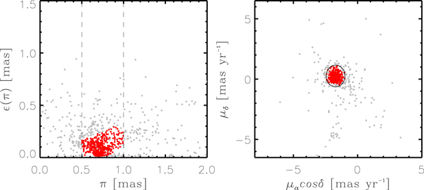
Figure 2. Parallax (left) and PM (right) distributions of member candidates (gray dots). Dashed lines in the left panel represent the lower and upper limits in parallax for selecting genuine members. The parallaxes from the Gaia EDR3 (Gaia Collaboration et al. 2021) are corrected for zero-point offsets (Lindegren et al. 2021). The ellipse in the right panel shows the region confined to 3.5 times the standard deviation from the weighted mean PMs, where the inverse of the squared PM error was used as the weight value. The selected members were plotted by red dots.
Download figure:
Standard image High-resolution imageFigure 3 shows the CMD of the selected members. A number of faint stars with large errors on parallax and PMs are naturally excluded through our member selection processes. The membership of these stars could be improved by the later release of the Gaia data. There is an X-ray source that was classified as a Class II YSO (the open circle in the upper panel of Figure 3). This object has a lower luminosity than those of the other members at a given color. An intermediate-mass YSO with a nearly edge-on disk could be a possible explanation for the low luminosity. However, such an object rarely shows X-ray emission and has low stellar mass (Sung et al. 2008, 2009). We therefore cautiously excluded this object from our member list. A total of 403 members were finally selected. We present the list of the members in Table 2.
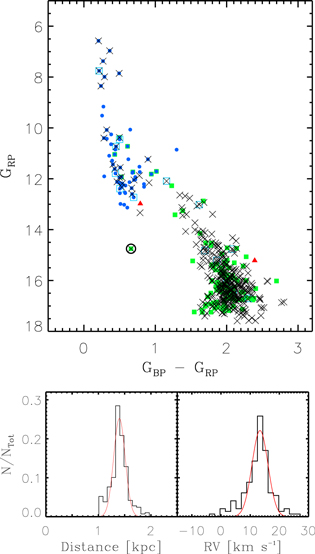
Figure 3. Selected members. The upper panel displays the CMD of the members taken from the photometric data of the Gaia DR2 (Gaia Collaboration et al. 2018). An open circle denotes a nonmember with an X-ray emission (see the main text for detail). The other symbols are the same as Figure 1. The lower left and lower right panels show the distance and RV distributions of the members, respectively. The distances were computed from the inversion of the recent Gaia parallaxes after correction for zero-point offsets (Gaia Collaboration et al. 2021; Lindegren et al. 2021). Red curves represent the best-fit Gaussian distributions.
Download figure:
Standard image High-resolution imageTable 2. List of Members
| Sq. | R.A. (2000) | Decl. (2000) | π |
|

|

| μδ |
| G |
| GBP |
| GRP |
| GBP − GRP | Early-type | YSO | X-ray | RV |
| Binarity flag |
|---|---|---|---|---|---|---|---|---|---|---|---|---|---|---|---|---|---|---|---|---|---|
| (h:m:s) | ( ) ) | (mas) | (mas) | (mas yr−1) | (mas yr−1) | (mas yr−1) | (mas yr−1) | (mag) | (mag) | (mag) | (mag) | (mag) | (mag) | (mag) | (km s−1) | (km s−1) | |||||
| 1 | 06:30:16.81 | +05:04:51.9 | 0.6459 | 0.0975 | −1.975 | 0.101 | 0.159 | 0.086 | 17.5846 | 0.0102 | 18.4017 | 0.0792 | 16.3339 | 0.0241 | 2.0677 | X | ⋯ | ⋯ | |||
| 2 | 06:30:26.49 | +05:02:41.1 | 0.9872 | 0.1871 | −2.220 | 0.216 | 0.014 | 0.173 | 18.6931 | 0.0044 | 19.2147 | 0.0372 | 17.2773 | 0.0173 | 1.9374 | X | ⋯ | ⋯ | |||
| 3 | 06:30:28.15 | +05:05:30.3 | 0.6576 | 0.1224 | −2.267 | 0.130 | 0.110 | 0.127 | 17.4778 | 0.0033 | 18.3454 | 0.0266 | 16.2546 | 0.0112 | 2.0908 | X | ⋯ | ⋯ | |||
| 4 | 06:30:30.87 | +05:00:49.3 | 0.5226 | 0.1168 | −1.855 | 0.129 | −0.044 | 0.104 | 17.6367 | 0.0019 | 18.7096 | 0.0176 | 16.3491 | 0.0070 | 2.3604 | X | 16.446 | 4.037 | |||
| 5 | 06:30:32.61 | +05:06:16.6 | 0.9460 | 0.1443 | −1.765 | 0.167 | −0.228 | 0.152 | 17.9478 | 0.0081 | 18.7829 | 0.0303 | 16.5876 | 0.0066 | 2.1953 | X | ⋯ | ⋯ | |||
| 6 | 06:30:41.00 | +04:57:30.9 | 0.7264 | 0.0720 | −1.737 | 0.083 | −0.214 | 0.067 | 16.9469 | 0.0081 | 17.8253 | 0.0296 | 15.7647 | 0.0251 | 2.0606 | X | 6.683 | 0.605 | |||
| 7 | 06:30:42.01 | +05:00:59.7 | 0.7461 | 0.0296 | −1.713 | 0.034 | −0.168 | 0.027 | 15.0324 | 0.0009 | 15.8159 | 0.0053 | 14.1195 | 0.0032 | 1.6965 | X | 18.709 | 0.468 | |||
| 8 | 06:30:44.15 | +05:02:21.0 | 0.6525 | 0.0871 | −1.957 | 0.092 | 0.223 | 0.075 | 17.0066 | 0.0043 | 17.9700 | 0.0145 | 15.8613 | 0.0107 | 2.1088 | X | 17.468 | 0.999 | |||
| 9 | 06:30:46.18 | +05:01:51.3 | 0.7509 | 0.0720 | −1.849 | 0.082 | 0.222 | 0.064 | 16.5845 | 0.0022 | 17.7197 | 0.0176 | 15.4415 | 0.0079 | 2.2782 | X | 21.966 | 4.375 | |||
| 10 | 06:30:46.77 | +04:59:04.2 | 0.5454 | 0.0441 | −1.810 | 0.050 | −0.108 | 0.040 | 15.8938 | 0.0028 | 16.7182 | 0.0105 | 14.9212 | 0.0069 | 1.7970 | X | 16.465 | 0.579 |
Note. Column (1): Sequential number. Columns (2) and (3): The equatorial coordinates of members. Columns (4) and (5): Absolute parallax and its standard error. Columns (6) and (7): PM in the direction of R.A. and its standard error. Columns (8) and (9): PM in the direction of decl. and its standard error. Columns (10) and (11): G magnitude and its standard error. Columns (12) and (13): GBP magnitude and its standard error. Columns (14) and (15): GRP magnitude and its standard error. Column (16): GBP − GRP color index. Column (17): Early-type members. “E” represents O- or B-type stars obtained from the data bases of MK classification (Mermilliod & Paunzen 2003; Reed 2003; Skiff 2009; Maíz Apellániz et al. 2013, SIMBAD). Column (18): YSO classification. “1,” “2,” and “T” denote Class I, Class II, and YSOs with a transitional disk, respectively. Column (19): X-ray source. “X” and “x” indicate X-ray source and X-ray source candidates, respectively. Columns (20) and (21): RV and its error. Columns (22): Binarity flag. “SB2” represents a double-line spectroscopic binary candidate. The parallax and PM were taken from the Gaia Early Data Release 3 (Gaia Collaboration et al. 2021), while the photometric data were obtained from the Gaia Data Release 2 (Gaia Collaboration et al. 2018). We corrected the zero-point offsets for the Gaia parallaxes according to the recipe of Lindegren et al. (2021). The full table is available electronically.
Only a portion of this table is shown here, to demonstrate its form and content. A machine-readable version of the full table is available.
Download table as: DataTypeset image
We compared our member list with that of Cantat-Gaudin et al. (2018). There are 238 stars in common with membership probabilities higher than 0.5. However, we suspect that their list contains a number of field interlopers below the locus of YSOs in CMD. They may be too old to be the members of this young SFR. Some giant stars were also selected as members. In addition, the member list is missing several O- and B-type stars that are the most likely members. For these reasons, we decided to use our own list of members.
We present the distance and RV distributions of the selected members in the lower panel of Figure 3. The distances of individual stars were computed via the inversion of the zero-point-corrected Gaia parallaxes (Gaia Collaboration et al. 2021; Lindegren et al. 2021). Since these two distributions appear as Gaussian distributions, the distance and systemic velocity of this SFR are obtained from the center of the best-fit Gaussian distributions. The distance is determined to be 1.4 ± 0.1 (s.d.) kpc. This is in good agreement with those derived by previous studies within errors (Ogura & Ishida 1981; Hensberge et al. 2000; Cantat-Gaudin et al. 2018; Kuhn et al. 2019). The systemic RV of this SFR is 13.4 ± 2.7 (s.d.) km s−1. To minimize the contribution of binaries, we limited the RV sample to stars with RVs within three times the standard deviation from the peak value.
4. Structures and Kinematics
Figure 4 displays the spatial distribution and surface density map of the members. The surface density map was obtained by counting stars with an interval of  along the R.A. and decl., where grids dithered by half the bin size were used to improve the spatial resolution. The central cluster NGC 2244 seems to have a substructure, as its surface density does not sharply drop toward the southeast. In addition to the cluster, there are at least three stellar groups with slightly enhanced peak surface densities (8% of the maximum density of NGC 2244) compared to nearby regions. The presence of the group (NGC 2237) at the western patch of the Rosette Nebula was reported by previous studies (Li 2005; Bonatto & Bica 2009; Wang et al. 2010). The small eastern group is found at the tip of the gas pillar on the east side of the nebula, and the other group corresponding to the known PL02 (Phelps & Lada 1997) is located at the southeastern molecular ridge.
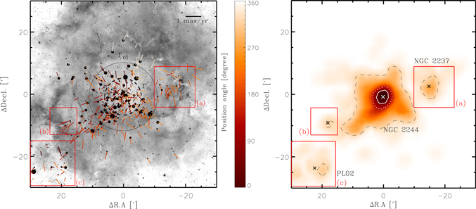
Figure 4. Spatial distribution (left) and surface density map (right) of members. The background image in the left panel was taken from the Digital Sky Survey image. The sizes of the dots are proportional to the brightnesses of individual stars in the GRP band. The PM vectors relative to the systemic motion are also plotted by solid line, and the different colors represent the position angle of the PM vectors as shown in the scale bar. The two circles (solid and dashed lines) indicate the apparent radius (rcl) and half-mass radius (rh), respectively. Red squares denote the locations of three subregions. In the right panel, white solid, white dotted, and black dashed lines represent contours corresponding to the 70%, 50%, and 8% levels of the maximum density, respectively. The squares correspond to the three subregions in the left panel. The crosses represent the centers of the four groups determined from median coordinates. The reference coordinate is the same as Figure 1.
Download figure:
Standard image High-resolution imageWe determined the central position and systemic motion of NGC 2244 in order to probe stellar motions relative to this cluster. The reference coordinate (R.A. = 06h 31m 5500, decl. = + 04°
 30
300, J2000) used in Figure 1 was adopted as the initial position of the cluster center. A new central position and systemic PM of NGC 2244 were obtained from the median coordinates and PMs of stars within a radius of
 . This procedure was repeated until these parameters converged to constant values. We found the cluster center at R.A. = 06h31m55
60, decl. =
 (J2000) and the systemic PM of
  = −1.731 mas yr−1, μδ
= 0.312 mas yr−1.
= −1.731 mas yr−1, μδ
= 0.312 mas yr−1.
4.1. NGC 2244
Figure 5 displays the radial surface density profile fit to the model profiles of Elson et al. (1987) in a logarithmic scale. The surface density of NGC 2244 decreases with the radial distance, but is influenced by NGC 2237 beyond the radius of  (see also the left panel of Figure 4). Therefore, we adopted this boundary as the apparent radius of NGC 2244 (rcl). This radius encompasses the majority of cluster members. The fundamental parameters and kinematics of this cluster were investigated within this radius.
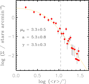
Figure 5. Radial surface density profile in logarithmic scale. The orange curve represents the best-fit model from Elson et al. (1987). The radius at which the western group begins to affect the surface density profile is indicated by a dashed line ( ).
).
Download figure:
Standard image High-resolution image4.1.1. Age
In order to derive the fundamental parameters (reddening, age, mass, and half-mass–radius) of this cluster, we fit the isochrones from MESA models considering the effects of stellar rotation (Choi et al. 2016; Dotter 2016) to the CMD. The distance modulus of 10.73 mag (equivalent to 1.4 kpc) was applied to the unreddened isochrones (AV = 0 mag). For the early-type members with colors bluer than GBP − GRP = 0.6, the reddening of the individual stars was obtained by fitting them to the distance-corrected isochrones along the reddening vector of Wang & Chen (2019) [AGRP/E(GBP − GRP) = 1.429]. The mean reddening is then estimated to be 〈E(GBP − GRP)〉 = 0.733 ± 0.078.
Figure 6 shows the CMD of the members in NGC 2244. The isochrones for four different ages (2, 3, 5, and 10 Myr) were superimposed on the CMD after correction for the mean reddening. Some B-type stars may be already evolving into the main sequence. The magnitude of the main-sequence turn-on is sensitive to the age of the cluster. The isochrone for 2 Myr well-matches the main-sequence turn-on. We adopt 2 Myr as the age of NGC 2244, and this is in good agreement with the previous estimates (Hensberge et al. 2000; Park & Sung 2002). However, the entire shape of the CMD seems to be fit by isochrones in a wide range of ages (ΔAge > 7 Myr). There could be systematic uncertainties in the calibration adopted in the theoretical models (Choi et al. 2016; Dotter 2016). Observationally, photometric errors, imperfect reddening correction, binaries, and variabilities of YSOs are possible sources of the observed scatter in the CMD (Lim et al. 2015). In addition, the luminosity spread can be caused by multiple star formation events.
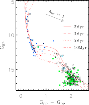
Figure 6. CMD of NGC 2244. Red curves are the isochrones from the MESA models (Choi et al. 2016; Dotter 2016) for 2, 3, 5, and 10 Myr. The arrow represents the reddening vector. The other symbols are the same as in Figure 1.
Download figure:
Standard image High-resolution image4.1.2. The Initial Mass Function and Total Stellar Mass
The mass function is important to estimate the total cluster mass, which allows us to infer the virial state of NGC 2244 at a current epoch. To derive the mass function of this cluster, we first obtained the masses of individual stars from the CMD by means of the isochrones from the MESA evolutionary models (Choi et al. 2016; Dotter 2016). The masses of early-type main-sequence members (GBP − GRP < 0.6) were obtained by interpolating their magnitude to the mass–luminosity relation constructed from the isochrones for 2, 5, and 10 Myr, where the individual reddening values were applied to the isochrones. For the other members, we adopted a mean reddening because the individual reddening values of these stars cannot be obtained from the current data. The colors of stars were interpolated to the grid of the isochrones with different ages (0.1–40 Myr) in order to construct the mass–luminosity relations at the given colors. The masses of individual members were then obtained from the interpolation of their magnitude to the mass–luminosity relations.
To compute the uncertainty in mass estimation, the photometric errors were added to or taken out from the observed magnitudes and colors. We then found the masses associated to these increased or decreased magnitudes and colors in the same way as done before. The mass uncertainties were adopted from half the difference between the upper and lower values. A typical uncertainty due to photometric errors is about 0.1M⊙. Differential reddening can also affect the mass estimation. The uncertainty in mass is then about 0.3 M⊙, on average, if we considered the differential reddening of 0.078.
We derived the present-day mass function of this cluster by counting the number of stars in given logarithmic mass bins ( ). A bin size of 0.2 was used to count the number of stars with mass smaller than 10 M⊙, while a larger bin of 1.08 was used for higher-mass stars because of their paucity. Then, the mass function was normalized by the associated bin sizes. To avoid the binning effects, we repeated the same procedure by shifting the bin size by half. The Poisson noise was adopted as the errors on the mass function.
Figure 7 displays the present-day mass function. The difference between the initial and present stellar masses is negligible in the first few Myr. According to the MESA model (Choi et al. 2016; Dotter 2016), the most massive star in NGC 2244 has lost 4M⊙ for 2 Myr. Hence, the present-day mass function can be considered as the initial mass function. We constrained the slope (Γ) of the mass function down to the turnover mass (∼1 M). The slope is estimated to be Γ = −1.4 ± 0.1 from a least-squares fitting method for stars with masses larger than 1 M⊙. This is in good agreement with those obtained from other SFRs in the solar neighborhood (Salpeter 1955; Kroupa 2001).
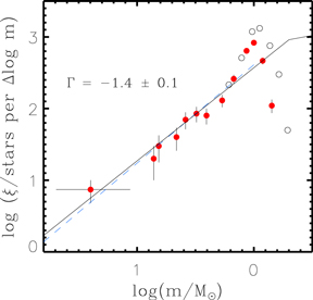
Figure 7. Present-day mass function of NGC 2244 (red dots). The result of a least-squares fitting to the mass function is shown by a blue dashed line. Black solid lines represent the Kroupa initial mass function (Kroupa 2001) for comparison. The open circles denote the upper limits of the mass function derived from members and member candidates fainter than 14 mag in GRP band.
Download figure:
Standard image High-resolution imageHowever, it does not guarantee that our member selection is complete down to the turnover mass. Since we selected the most likely members using strict selection criteria, many lower-mass members with large errors in parallax and PM may have been excluded. We estimated the upper limits of the mass function including member candidates fainter than 14 mag in GRP band in the same way as above (open circles in Figure 7). The upper limits follow a trend similar to the original one for masses larger than 1 M⊙ and become larger for the lower-mass regime. The number of stars obtained from the original mass function is about 30% lower than that from the upper limits at around the turnover mass. However, this may not be the actual completeness limit of our sample, because some field interlopers may be included in the sample of member candidates. If we adopt the upper limits of the mass function, then the slope of the mass function is estimated to be Γ = −1.6 ± 0.2, which is consistent with the value found above within errors.
The sum of the stellar masses yields a total mass of 533 M⊙. However, this result does not consider a number of stars with very low mass (<1 M⊙). In order to infer their population, we scaled the Kroupa initial mass function to ours (the original mass function) using the mean difference between these mass functions. This scaled Kroupa initial mass function was then integrated in the mass range of 0.08 M⊙ to 1 M⊙. The number of cluster members down to the hydrogen-burning limit is expected to be about  , where the upper and lower limits were inferred from the integration of the scaled Kroupa initial mass functions adjusted by the uncertainty of the scaling factors (i.e., the standard deviation) in the low-mass regime (<1 M⊙). The total stellar mass of NGC 2244 is estimated to be about 879
 M⊙, which is slightly larger than those previously obtained by other studies (770M⊙—Pérez 1991; 625M⊙—Bonatto & Bica 2009).
We also estimated a projected half-mass radius (rh) of  (equivalent to 2.4 pc) from our limited sample. A recent study derived the initial mass function of stars in a very small central region, down to the subsolar mass regime (Mužić et al. 2019). The mass function appeared similar to the Kroupa initial mass function, which implies that there is no sign of dynamical mass segregation. Hence, rh obtained in this study may not be significantly altered even if the radial mass distribution of stars in the full mass range is considered.
4.1.3. Internal Kinematics
The PM vectors of the members relative to the systemic motion of NGC 2244 are shown in Figure 4. Stars in the central cluster show outward motions, which were also detected in Kuhn et al. (2019). To probe the direction of their motion in detail, we calculated the vectorial angle (Φ) between the position vectors from the cluster center and the relative PM vectors of stars (see also Lim et al. 2019, 2020). A Φ close to 0° means that a given star is radially moving away from the center of the cluster, while a Φ of 180° indicates that the star is moving toward the cluster center.
Figure 8 displays the Φ distribution of stars in NGC 2244. The cluster members have Φ values in a wide range. We present the histograms of Φ values in the right panel of the figure. There is a peak at 0°, which indicates that some stars are radially escaping from NGC 2244. Given that this feature seems weaker within rh (blue open squares in the figure), the majority of these escaping stars may be distributed beyond rh.
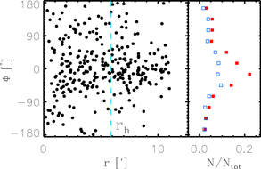
Figure 8. The Φ distribution of stars in NGC 2244. The dashed line in the left panel represents rh of this cluster. Red filled squares and blue open squares exhibit the histograms of Φ values for all stars and only stars within rh, respectively.
Download figure:
Standard image High-resolution imageIn order to search for the signature of cluster rotation, the RV distribution of stars was investigated as addressed in many previous studies (Lane et al. 2009; Mackey et al. 2013). We first considered a projected rotational axis across the cluster center from north (0°) to south (180°). The difference between the mean RVs of stars in the two regions separated by the projected rotational axis was computed. The same procedure was repeated for various position angles of the projected rotational axis with an interval of 20°.
We found a variation of the mean differences of RVs with the position angles of the projected rotational axis, as shown in the left panel of Figure 9. This variation was fit to the sinusoidal curve as below:

where Vrot, i, and ϕ0 represent the rotational velocity, inclination of a rotational axis, and phase, respectively. The amplitude of the sinusoidal curve corresponds to twice the projected rotational velocity ( ). The position angle of the projected rotational axis can be inferred from 270° − ϕ0. The projected rotational axis is tilted by ∼20° (±14°) from north to east. We investigated a variation of
  using stars within various radii from
  to
to  . The middle panel of Figure 9 displays the variation of
  with the projected radial distances. In the inner region (<6
5),
 of stars increases up to 0.67 km s−1 with the radial distance, and drops to ∼0.20 km s−1 beyond this radius. It is interesting that this cluster rotation is evident around rh. A clear pattern of cluster rotation is also seen in the position–velocity diagram (the right panel of Figure 9).
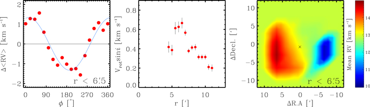
Figure 9. Signature of cluster rotation. Left panel: differences of mean RVs with respect to the position angles of the projected rotational axis within  (2.6 pc). The blue solid line represents the best-fit sinusoidal curve. The projected rotational velocity can be estimated from the amplitude of the sinusoidal curve divided by 2. Middle panel: variation of projected rotational velocities with respect to the radial distances. The dots and error bars were obtained from the best-fit sinusoidal curves for different samples. Right panel: spatial distribution of mean RVs within
  . The color bar shows the different levels of mean RVs. The mean RVs were computed within spatial bins of
  . A grid dithered by half the bin size was used to sample the stars. The cross indicates the center of NGC 2244. The reference coordinate is the same as Figure 1.
Download figure:
Standard image High-resolution imageThe signature of cluster rotation was also searched for using PMs. The one-dimensional tangential velocities (Vt) of stars along R.A. and decl. were calculated by adopting a distance of 1.4 kpc. Since the diameter of the cluster is very small compared to the distance, the error on Vt by the extent of the cluster is less than 1% under the assumption that this cluster has a spherical shape. The rotational velocity on the celestial sphere is given by the equation below:

where r, dR.A., VR.A, ddecl., and Vdecl. represent the radial distance, the position and Vt in R.A., and the position and Vt in decl., respectively. The nonzero mean velocity would yield the rotational velocity of this cluster. However, the mean velocity was calculated to be 0.03 ± 1.32 km s−1, meaning that this cluster does not have significant azimuthal motion. This result is consistent with that found by Kuhn et al. (2019). Since the cluster rotation was only detected in RV, the rotational axis of NGC 2244 may be tilted by almost 90° from the line of sight.
4.1.4. Dynamical State
We computed the virial velocity dispersion of NGC 2244 by using the equation (Parker & Wright 2016) below:

where G, Mtotal, R, and η represent the gravitational constant, enclosed total mass, radius, and the structure parameter, respectively. Note that we can consider the total cluster mass of 879 M⊙ as the enclosed mass, given that gas has already been removed around NGC 2244 according to 12CO (J = 1 − 0) and 13CO (J = 1 − 0) observations (Heyer et al. 2006). The rh of 2.4 pc was used in Equation (4). The structure parameter η has a value between 1 and 12 depending on the geometry of the cluster. Here, η of 10 was adopted because the observed surface density profile (γ = 3.5 ± 0.3; Figure 5) is close to that (γ = 4) of Plummer (1911; see also Figure 4 of Portegies Zwart et al. 2010). The expected velocity dispersion at a virial state is about 0.6 km s−1 (for reference, the virial velocity dispersion for other clusters is in the range of 0.4–1.6 km s−1; see Kuhn et al. 2019). The virial velocity dispersion is not very sensitively varied with the total mass, because it is proportional to  . The virial velocity dispersion is almost constant even if we adopted the upper limit of the total cluster mass.
Figure 10 displays the distributions of VR.A, Vdecl., and RV (the upper panels) with their error distributions (the lower panels). We derived the systemic velocities and velocity dispersions from the best-fit Gaussian distributions (Table 3). The typical errors on the measurements are estimated from the weighted-mean errors, where the associated error distributions were used as the weight values for given errors. We obtained the intrinsic velocity dispersions of 0.8 and 0.8 km s−1 along R.A. and decl., respectively, from quadratic subtraction between the observed velocity dispersions and their typical errors. The effect of system rotation on the observed RV dispersion can be simulated by using the ideal Gaussian velocity distribution based on the underlying rotation with position angles. As a result, the observed velocity dispersion can be inflated by about 14% compared to the intrinsic velocity dispersion. Since our measurement of the velocity dispersion along the line of sight, after quadratic subtraction by the typical error of 1.6 km s−1, is about 0.8 km s−1, the intrinsic RV dispersion would be 0.7 km s−1. The mean value from the intrinsic velocity dispersions along R.A., decl., and the line of sight is 0.8 ± 0.1 km s−1.
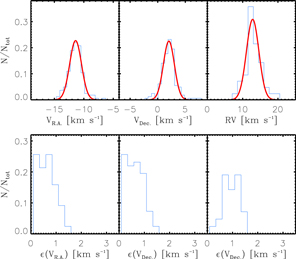
Figure 10. Velocity (upper) and error (lower) distributions along R.A., decl., and the line of sight. The histograms were obtained from stars within rh using bin sizes of 0.6, 0.6, and 1.5 km s−1 for VR.A, Vdecl., and RV, respectively. The red curves represent the best-fit Gaussian distributions. The systemic velocities and velocity dispersions are presented in Table 3. In the lower panels, the associated errors were sampled with a bin size of 0.25 km s−1.
Download figure:
Standard image High-resolution imageTable 3. Velocity Dispersions
| Vsys | σobs | σerr | σint | |
|---|---|---|---|---|
| (km s−1) | (km s−1) | (km s−1) | (km s−1) | |
| VR.A | −11.4 | 1.0 | 0.6 | 0.8 |
| Vdecl. | 2.0 | 1.0 | 0.6 | 0.8 |
| RV | 12.8 | 1.8 | 1.6 | 0.7 a |
Notes. Velocity dispersions were obtained for members within rh . Columns (2)–(4) represent the systemic velocities, the observed velocity dispersions, typical errors, and the intrinsic velocity dispersions along R.A, decl., and the line of sight, respectively.
a The contribution of the cluster rotation (14%) has been corrected for the RV dispersion.Download table as: ASCIITypeset image
The initial size of this cluster might have been smaller than the current one. In addition, a large amount of the natal cloud mass probably remained around the cluster. The virial velocity dispersion might have thus been larger than what we derived. While the velocities of cluster members at a supervirial state are not significantly altered in the first several Myr (Schoettler et al. 2019), the virial velocity dispersion could decrease with the evolution of the cluster because of the cluster expansion and gas expulsion. At the current epoch, the observed velocity dispersion is comparable to  times the virial velocity dispersion, which implies that the total kinetic energy is almost in balance with the total potential energy. This cluster may be gravitationally unbound. The weak pattern of expansion within rh supports this argument.
The relaxation time of this cluster was estimated from the equation of Binney & Tremaine (1987). The crossing time of stars for rh is about 2.9 Myr, adopting the mean velocity dispersion of 0.8 km s−1. Given the total number of stars (1510), the dynamical relaxation time was estimated to be about 76 Myr. The age of NGC 2244 is much younger than this timescale, and therefore dynamical mass segregation may not be found in this cluster. Figure 11 displays the two-dimensional Vt ( ) distribution with respect to the radial distance and stellar mass. Since dynamical mass segregation is the result of energy equipartition (Binney & Tremaine 1987), the signature of this dynamical process can be probed from a correlation between stellar mass and velocities, i.e., the low-mass stars have velocities higher than those of high-mass stars. However, there is no evidence for the energy equipartition among cluster members, confirming the result of Chen et al. (2007). Furthermore, the most massive O-type stars are widely distributed across the cluster region.
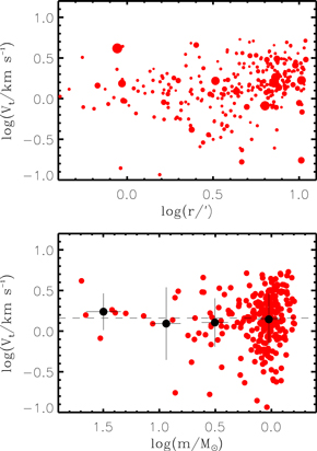
Figure 11. Two-dimensional Vt distribution of cluster members with respect to the radial distance (upper) and stellar mass (lower). In the upper panel, the sizes of the dots are proportional to the masses of individual stars. The dashed line in the lower panel represents the median Vt. Dots and error bars denote the mean and standard deviations of masses and Vt within a given logarithmic mass bin of 0.5, respectively.
Download figure:
Standard image High-resolution image4.2. Stellar Groups around NGC 2244
The physical association between stellar groups and remaining gas can be a key clue to understanding the formation of substructures. Toward this aim, the distributions of stars and gas were investigated in position–velocity space. We constructed a three-dimensional position–position–velocity diagram of ionized gas as made in our previous studies (Lim et al. 2018, 2019). A data cube composed of 90 × 90 × 90 regular volume cells was created, and then a Delauney triangulation technique was used to interpolate the intensities and velocities of the forbidden line [N ii] λ6584 into the individual cells. From this data cube, we also obtained position–velocity diagrams by the sum of the counts along R.A. and decl., respectively. The positions and RVs of stars are overplotted in these diagrams.
Figure 12 shows the distribution of stars and ionized gas in position–velocity space. A cavity of the H ii region is clearly seen in the central region occupied by NGC 2244 (red). In the position–velocity diagrams, the other stellar groups (blue) are found along the H ii bubble, and they have velocities roughly similar to those of the ionized gas. This indicates that these groups and remaining gas belong to the same physical system. The RVs of ionized gas range from 0 to 30 km s−1, and therefore the Rosette Nebula is expanding at velocities up to 17.2 km s−1 from NGC 2244 (12.8 km s−1; Table 3).
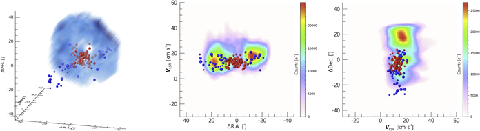
Figure 12. Distribution of stars and ionized gas in position–velocity diagrams. Stars in the NGC 2244 region are plotted by red spheres, and the other stars are shown by blue spheres. The sizes of the spheres are proportional to the brightnesses of individual stars in the GRP band. Left panel: position–position–velocity diagram. The bluish nebula represents the distribution of ionized gas traced by the forbidden line [N ii] λ6584. Middle and right panels: position–velocity diagrams along R.A. and decl., respectively. Contour shows the integrated intensity distribution of [N ii] λ6584 line in unit of electrons (e−). The reference coordinate is the same as Figure 1.
Download figure:
Standard image High-resolution imageIn order to find the physical association between stellar groups and gas, it is necessary to probe them in detail in smaller position–velocity space. We investigated the three stellar groups that are likely associated with adjacent gas structures (the left panel of Figure 4). An amount of molecular gas still remains in the vicinity of these groups. Figure 13 exhibits the distribution of stars on the integrated intensity maps and position–velocity diagrams of molecular gas. The RVs of ionized gas measured from the [N ii] λ6584 were also superimposed on the figure. The ionized and molecular gas appear to have similar RVs.
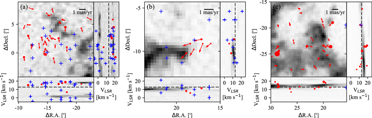
Figure 13. Integrated intensity maps and position–velocity diagrams obtained from the 12CO (J = 1 − 0) line. Panels (a) to (c) correspond to the regions indicated by boxes in the left panel of Figure 4. The distribution of molecular gas is plotted in gray scale. Red dots represent the positions and RVs of stars, and their sizes are proportional to their brightnesses. Arrows denote the PM vectors relative to the systemic motion of NGC 2244. Fiber positions used to obtain optical spectra as well as RVs of ionized gas are shown by pluses. The sizes of the errors on RV are smaller than the symbol size. The dashed lines in the position–velocity diagrams represent the systemic velocity of this SFR. The reference coordinate is the same as Figure 1.
Download figure:
Standard image High-resolution imageMost stars in subregion (a) may be members of the neighboring cluster NGC 2237 (Li 2005; Wang et al. 2010). There are two gas components in the position–velocity diagrams, which is indicative of expanding shell components. The ionized gas also traces both components in RV. The heads of the gas pillars seen in the left panel of Figure 4 correspond to the molecular gas clumps at (ΔR.A., Δdecl.) ∼( ,5
,5 ). The RVs of these clumps range 0–5 km s−1. Given the systemic velocity of NGC 2244 (12.8 km s−1), they may be part of the near side of the H ii bubble. Some gas structures associated with this bubble extend southwest. This component may be expanding at velocities up to −12.8 km s−1, although this is a projected expanding velocity. The other gas component is found at (ΔR.A., Δdecl.) ∼(
 ,1
,1 ) and has RVs in a range of 15–20 km s−1. This component may be part of the bubble receding away from NGC 2244 at projected velocities up to 7.2 km s−1. NGC 2237 is located in the vicinity of the heads of the gas pillars. Most stars in this group tend to systematically move toward the south. Stars with RV measurements have RVs in range 15–21 km, except for one star. Therefore, this group seems kinematically associated with the latter gas component, rather than the gas pillars.
There is a gas pillar in subregion (b). This gas structure is moving at velocities of about 10 km s−1 along the line of sight, which is smaller than the systemic velocity of NGC 2244 (12.8 km s−1). It implies that this is part of the near side H ii bubble approaching observers. There is a small group of stars in the vicinity of the gas pillar. These stars have RVs similar to that of the gas pillar, although the number of stars with RV measurements is only three out of six. In addition, their PM vectors are systematically oriented toward the southeast (i.e., away from the central cluster).
The remaining gas in subregion (c) is part of the northwestern ridge of the Rosette Molecular Cloud. This molecular gas has RVs slightly larger than the systemic velocity of the central cluster, and therefore it is receding away from the cluster in the line of sight. There are more than 20 members of PL02 in the subregion. Their RVs range from 7 to 19 km s−1. It is unclear whether or not PL02 is physically associated with this gas, due to the spread of the RVs. Given that the PM vectors of the PL02 members are small and random, the velocity field of this group may be closer to that of NGC 2244 than that of the molecular gas.
5. Discussion
5.1. The Formation of NGC 2244
The formation of stellar clusters has been explained by two scenarios: monolithic formation (Kroupa et al. 2001; Banerjee & Kroupa 2013, 2015) and hierarchical mergers of subclusters (Bonnell et al. 2003; Bate 2009). Cluster rotation can also provide additional implications with regard to the cluster formation (Corsaro et al. 2017; Mapelli 2017). Here, we discuss the formation of the central cluster NGC 2244 in the two-theories framework.
Stellar clusters may form along the dense regions in a turbulent molecular cloud because star formation efficiencies can be high in this environment (Kruijssen 2012). Recent simulations of monolithic cluster formation have been capable of reproducing the internal structures and kinematics of clusters (Kroupa et al. 2001; Banerjee & Kroupa 2013, 2015; Gavagnin et al. 2017). Rapid gas expulsion and stellar feedback can significantly change the structure and kinematics of clusters (Tutukov 1978; Hills 1980; Lada et al. 1984; Kroupa et al. 2001; Banerjee & Kroupa 2013, 2015; Gavagnin et al. 2017). However, it is also possible to explain the formation of stellar clusters even without consideration of these effects. Our previous study (Lim et al. 2020) simulated the dynamical evolution of a model cluster formed in an extremely subvirial state. This model cluster collapses in the first several million years and expands. Subsequently, its structural features and kinematics were compared with those of the young open cluster IC 1805 (3.5 Myr—Sung et al. 2017) composed of a virialized core and an expanding halo. The model cluster had properties that compared well with the observed structure and kinematic properties of IC 1805.
Many other clusters in OB associations also tend to show expansion (Cantat-Gaudin et al. 2019; Kuhn et al. 2019), but it seems difficult to detect cluster rotation by using only PMs, as rotating clusters are rare in the sample of Kuhn et al. (2019). However, the rotation of NGC 2244 was found via RVs in this study. Therefore, the spectroscopic observations are crucial to perform a more complete search of cluster rotation. Indeed, the significant rotation of the young massive cluster R136 in the Large Magellanic Cloud was detected from spectroscopic observations (Hénault-Brunet et al. 2012). The rotational energy accounts for more than 20% of total kinetic energy of this cluster. The detection of cluster rotation implies that clusters can form in rotating molecular clouds or from hierarchical mergers of small stellar groups with different motions.
Systematic survey of molecular clouds in external galaxies found that molecular clouds are rotating (Rosolowsky et al. 2003; Tasker 2011; Braine et al. 2020). More than 50% of the observed molecular clouds have prograde rotation with respect to the galactic rotation. The angular momenta of these clouds may be acquired from the differential rotation of disk and self-gravity. The clouds with retrograde rotation can form via cloud–cloud collisions (Dobbs et al. 2011). The rotation of stellar clusters can thus be inherited from their natal clouds. However, it is not yet understood how efficiently the angular momenta of their natal clouds are redistributed to individual stars and clusters.
The hierarchical merging of gaseous and stellar clumps in a turbulent cloud can also lead to the formation of rotating clusters (Mapelli 2017). There are some possible candidates. The core of 30 Doradus in the Large Magellanic Cloud has an elongated shape, and it is composed of two stellar populations with different ages (Sabbi et al. 2012). The dense group is known to be the young massive cluster R136, which presents rotation (Hénault-Brunet et al. 2012), while a diffuse stellar group is located at the northeast of this cluster. It is believed that the elongated structure and age difference indicate a recent or an ongoing merger of these two groups (Sabbi et al. 2012). Similarly, the young massive cluster Westerlund 1 has an elliptical shape (Gennaro et al. 2011) and hosts two different age groups (Lim et al. 2013). However, the rotation of this cluster has not been reported yet.
NGC 2244 could monolithically form in a rotating cloud or filament hub, after which it might undergo cold collapse depending on its initial virial state. Some stars are now escaping from the cluster, as seen in Figure 8. Gas expulsion may also play a role in dispersing the cluster members. In addition, there are several stars in the north and south beyond rcl, and these stars are also moving away from the cluster (see Figure 4). We traced their positions back using PMs. As a result, about 85% (11/13) of these stars were in the cluster (<rcl) 2 Myr ago. Therefore, the spatial distribution of these stars can also be explained by the dynamical evolution of this cluster after the monolithic formation.
The observed features in IC 1805 could be explained by the monolithic collapse and rebound (Lim et al. 2020). In the same context, we compare the pattern of expansion in NGC 2244 with those in IC 1805. While IC 1805 shows a strong expansion pattern in its outer region (Lim et al. 2020), NGC 2244 has, in comparison, a rather weak tendency toward expansion (Figure 8). One possible explanation would be that the initial rotation supported the system against the subvirial collapse. Dynamical mass segregation is a natural consequence of the violent relaxation during the cold collapse (Allison et al. 2009). However, the absence of notable mass segregation in NGC 2244 also implies that the cluster did not have a strong cold collapse in the past.
The western half of the cluster has a negative net RV relative to the systemic velocity as it rotates (Figure 9), while NGC 2237 has a positive net RV (Figures 12 and 13). The discrepancy between the directions of the cluster rotation and stellar motions in the subregion cannot be simply explained by the monolithic cluster formation in a rotating cloud. On the other hand, star formation is still taking place along the filaments in the Rosette Molecular Cloud, forming several groups of stars (Poulton et al. 2008; Schneider et al. 2010; Cambrésy et al. 2013). In particular, a clustering of the stellar groups PL04, PL05, PL06, and REFL08 is noteworthy (Cambrésy et al. 2013; see also Cluster E in Poulton et al. 2008). This circumstance is a favorable condition for merging of stellar groups. Similarly, NGC 2244 has a substructure toward the southeast (Figure 4). The structural feature and rotation of this cluster may be the result of hierarchical mergers of stellar groups.
5.2. The Origin of the Stellar Population around NGC 2244
The Herschel observation reveals that the Rosette Molecular Cloud is being affected by the ultraviolet irradiation from the massive stars in NGC 2244 (Schneider et al. 2010). A gradient of dust temperature was found toward the southeast. The age differences among individual stellar groups indicate the presence of an age sequence among YSOs from the H ii bubble toward the Rosette Molecular Cloud. Schneider et al. (2010) argued that the formation of the stellar groups may be triggered by the radiative feedback from massive stars in NGC 2244.
However, this argument was later refuted by Cambrésy et al. (2013). They measured the slope of spectral energy distributions of individual YSOs and better estimated the ages of the stellar groups. The stellar groups close to the Rosette Nebula are systematically younger than NGC 2244. On the other hand, the stellar groups PL06 and PL07 are far from the Rosette Nebula, but their ages are comparable to that of NGC 2244. As a conclusion, their age distribution could not be fully understood in the context of the feedback-driven star formation (Elmegreen & Lada 1977). Star formation in the Rosette Molecular Cloud seems to take place in two different ways (Phelps & Lada 1997). Several previous studies have also reached similar conclusions regarding the formation of these stellar groups (Poulton et al. 2008; Román-Zúñiga. et al. 2008; Ybarra et al. 2013).
To understand the formation of the three groups that we defined at the border of the Rosette Nebula (the left panel of Figure 4), it is necessary to consider both models of hierarchical star formation along filaments (Bonnell et al. 2011) and feedback-driven star formation (Elmegreen & Lada 1977) as suggested by Phelps & Lada (1997). Figure 14 displays the distributions of Tex and column density along the remaining molecular gas in these subregions. The heads of gas pillars in subregion (a) have Tex and column densities lower than those in the other subregions. The column density traced by the optically thin 13CO line compared to 12CO line shows no agglomeration deeper inside the pillar heads.
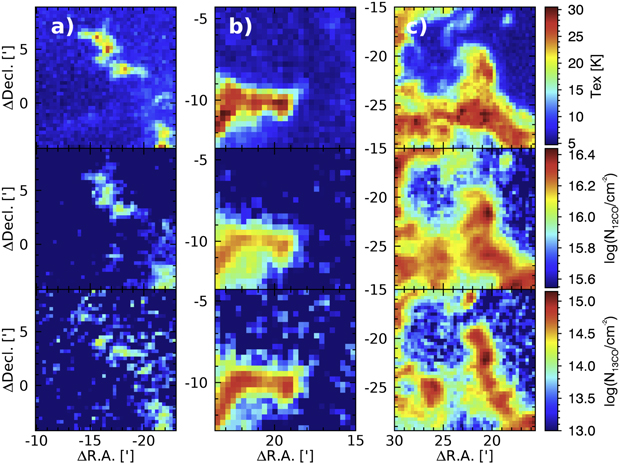
Figure 14. Distributions of Tex and column density in subregions (a) (left), (b) (middle), and (c) (right). The levels of Tex and column density are shown by the color bars. To minimize the contribution of diffuse gas toward this SFR (Heyer et al. 2006), the velocity ranges were limited to −3.0–10.0 km s−1 for subregion (a), 4.0–15.0 km s−1 for (b), and 6.0–18.5 km s−1 for (c). The reference coordinate is the same as Figure 1.
Download figure:
Standard image High-resolution imageA large amount of molecular gas still remains in subregions (b) and (c). Tex in subregions (b) and (c) appears higher than 25 K, which is consistent with dust temperature (Schneider et al. 2010). The molecular gas in subregion (b) condenses along the midplane, and a local condensation is found at the ridge of the molecular gas in subregion (c). These results indicate that molecular gas is compressed along the ridge of the Rosette Molecular Cloud because the clouds are exposed to the ultraviolet irradiation from the O-type stars in NGC 2244. Hence, subregions (b) and (c) might be the possible sites of feedback-driven star formation, compared to subregion (a). If PL02 is physically associated with the adjacent molecular gas, its age being younger than NGC 2244 (Cambrésy et al. 2013) may support this argument.
Here, we discuss the formation of the three groups based on their kinematics as shown in Section 4.2. If stars form in the remaining gas compressed by the expanding H ii bubble, it is expected that they are receding away from ionizing sources in NGC 2244 and have similar velocities to that of the gas. The stars in subregion (b) seem to follow this expectation. These stars are moving away from the cluster (toward the southeast) and have RVs similar to that of the adjacent gas pillar. In addition, this group contains a low-mass Class I YSO at an early evolutionary stage of protostars. This group may be slightly younger than the other groups, and hence its formation might be triggered by the feedback from massive stars in NGC 2244. We note that there is another Class I object in NGC 2244, but this may be a slightly old Herbig Ae/Be star candidate with a thick disk (Figure 6).
NGC 2237 in subregion (a) does not show any physical association between stars and the gas pillars (Figure 13). Also, this group is moving toward the south instead of the west (the direction of radial expansion of the H ii bubble). This confirms that region (a) is probably not a site of feedback-driven star formation. Although subregion (c) was considered as a possible site of feedback-driven star formation in Phelps & Lada (1997), the kinematic properties of PL02 and adjacent clouds do not support the claim. If PL02 was formed by the compression of the clouds, the members of PL02 should show PMs systematically receding away from NGC 2244. However, they have almost random motions, rather than any systematic motion toward the southeast as seen in subgroup (b). In addition, the physical association between PL02 and the remaining clouds is unclear. Hence, the formation of this group seems not to be related to feedback from the massive stars in the cluster. These two groups, NGC 2237 and PL02, might have been independently formed through the hierarchical fragmentation of a molecular cloud.
6. Summary
Stellar associations are not only ideal targets to understand star formation process on different spatial scales, but also the factories of field stars in the Galactic thin disk. There are three theoretical models to explain the formation of these young stellar systems, but our observational knowledge of their formation is still incomplete. In this study, we investigated gas and young stellar population in the Rosette Nebula, the most active SFR in the Mon OB2 association.
We identified the young star members based on photometric and spectroscopic criteria, complemented by parallax and proper motion criteria based on the recent Gaia astrometric data (Gaia Collaboration et al. 2021). A total of 403 stars were selected as the members. Their spatial distribution showed that this SFR is highly substructured.
The central cluster NGC 2244 is the most populous group in the Rosette Nebula. The age of this cluster was estimated to be about 2 Myr by means of stellar evolutionary models (Choi et al. 2016; Dotter 2016). We derived its mass function, which appeared to be consistent with the Salpeter/Kroupa initial mass function (Kroupa 2001) for stars with masses larger than 1 M⊙. However, a number of bona fide members with smaller masses could have been excluded because of our strict criteria of member selection. The total number of members and cluster mass were deduced to be about 1510 and
and  , respectively. This cluster showed a clear pattern of expansion beyond the rh (2.4 pc) and rotation below that radius. We also investigated correlations between stellar mass, velocity, and the radial distance of stars, but could not find any sign of dynamical mass segregation.
Several groups of stars were found at the border of the Rosette Nebula. We investigated the kinematic properties of stars in three subregions by comparing their RVs with those of adjacent gas structures. The eastern group (subregion (b)) seemed to be physically associated with the gas pillar and receding away from the central cluster. In addition, a low-mass Class I object was found in this group. These results can be understood in the context of feedback-driven star formation (Elmegreen & Lada 1977). On the other hand, there was no kinematic evidence of feedback-driven star formation in other subregions. These groups might have originated from spontaneous star formation along filaments.
In conclusion, all the processes proposed by the three theoretical models seem to be involved in the formation of this association. We need to examine other Galactic OB associations with the same perspective as that of this study. A systematic survey of both stars and gas in many stellar associations will provide key clues to understanding their formation process.
The authors thank the anonymous referee for many comments and suggestions. The authors would also like to express thanks to Professor Mark Heyer for providing supplementary data, Dr. Nelson Caldwell, and ShiAnne Kattner for assisting with Hectochelle observations. Observations reported here were obtained at the MMT Observatory, a joint facility of the University of Arizona and the Smithsonian Institution. In addition, this paper has made use of data obtained under the K-GMT Science Program (PID: MMT-2019B-1) funded through the Korean GMT Project operated by the Korea Astronomy and Space Science Institute (KASI) and from the European Space Agency (ESA) mission Gaia (https://www.cosmos.esa.int/gaia), processed by the Gaia Data Processing and Analysis Consortium (DPAC, https://www.cosmos.esa.int/web/gaia/dpac/consortium). Funding for the DPAC has been provided by national institutions, in particular the institutions participating in the Gaia Multilateral Agreement. The Digitized Sky Surveys were produced at the Space Telescope Science Institute under U.S. Government grant NAG W-2166. The images of these surveys are based on photographic data obtained using the Oschin Schmidt Telescope on Palomar Mountain and the UK Schmidt Telescope. The plates were processed into the present compressed digital form with the permission of these institutions. This paper also made use of data products from the Wide-field Infrared Survey Explorer, which is a joint project of the University of California, Los Angeles, and the Jet Propulsion Laboratory/California Institute of Technology, funded by the National Aeronautics and Space Administration. IRAF was distributed by the National Optical Astronomy Observatory, which was managed by the Association of Universities for Research in Astronomy (AURA) under a cooperative agreement with the National Science Foundation. This work was supported by the National Research Foundation of Korea (NRF) grant funded by the Korean government (MSIT; grant No: NRF-2019R1C1C1005224). Y.N. acknowledges support from the Fonds National de la Recherche Scientifique (Belgium), the European Space Agency (ESA), and the Belgian Federal Science Policy Office (BELSPO) in the framework of the PRODEX Programme (contracts linked to XMM and Gaia). J.H. acknowledges support from the Basic Science Research Program through the NRF funded by the Ministry of Education (No. 2020R1I1A1A01051827). N.H. acknowledges support from the Large Optical Telescope Project operated by KASI. B.-G.P. acknowledges support from the K-GMT Project operated by KASI.
Facility: MMT (Hectochelle). -
Appendix A: YSO Classification
The Spitzer IRAC and MIPS 24 μm observations of young stars in the Rosette Nebula were carried out by Balog et al. (2007). This survey covers an optically visible 30′ × 30′ region in the center of the nebula. We took their photometric data of 1084 stars detected in all four IRAC bands. Figure A1 displays the color–color diagrams of stars in mid-infrared wavelengths. Some stars have photospheric colors close to zero, while the others exhibit significant mid-infrared excess originating from their warm circumstellar disks or envelopes.
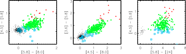
Figure A1. Color–color diagrams of stars in the Rosette Nebula obtained from Balog et al. (2007). Red triangles, green squares, cyan open squares, and black dots represent Class I, Class II, YSOs with transitional disks, and stars without any infrared excess emission, respectively.
Download figure:
Standard image High-resolution imagePrior to YSO classification, we flagged the sources of contamination. Active galactic nuclei (AGNs) and star-forming galaxies are also sources with infrared excess emission (Donley et al. 2008). These objects were identified by using the criteria of Gutermuth et al. (2008). A total of 104 AGNs and four star-forming galaxy candidates were found. One source was identified as a blob of shock emission that appears bright in 4.5 μm (Smith et al. 2006; Gutermuth et al. 2008).
The YSO candidates were identified from these CMDs according to the classification scheme of Gutermuth et al. (2008). We classified ten and 262 young stars as Class I and Class II objects, respectively. In addition, a total of 19 YSOs with a transitional disk were found in the color–color diagram combined with MIPS 24 μm photometry. Balog et al. (2007) identified 337 Class II and 25 Class I objects from the IRAC color–color diagrams and 213 Class II and 20 Class I objects from the IRAC and MIPS 24 μm photometry. The results of their YSO classification were different from ours for the same data. One reason may be due to the adoption of different classification schemes for AGNs, star-forming galaxies, and YSOs. The second possible reason is that Balog et al. (2007) published only the good-quality photometric data of sources detected in the four IRAC bands, and so it is possible that faint sources were omitted from their data. It is worth noting that such faint YSOs would not be selected as final members, because of their low-quality astrometric data (see Section 3).
The AllWISE catalog (Cutri et al. 2013) was used to identify more YSOs spread over the Rosette Nebula (a 6° × 6° region centered at R.A. = 06h 31m 5500, decl. = +04° 56′ 30
0, J2000). All YSOs and the other sources were classified according to the scheme of Koenig & Leisawitz (2014). This catalog contains a large number of spurious sources. All the criteria examined by Koenig & Leisawitz (2014) were applied to minimize the contamination by these spurious sources. The candidates of AGNs and star-forming galaxies were then sorted out from the color–magnitude cuts. Class I, Class II, and YSOs with a transitional disk were identified from color–color diagrams (Figure A2). Among these young stars, the candidates of asymptotic giant branch stars and classical Be stars were excluded in the list of YSO. In the end, we found a total of six Class I, 76 Class II, and two YSOs with transitional disks. Among them, a total of 40 YSO candidates were found in the field of view of the Spitzer observation (Balog et al. 2007). This number is lower than that identified from the Spitzer data because of the lower sensitivity of the WISE mission (Wright et al. 2010).
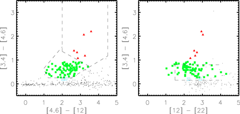
Figure A2. Color–color diagrams of stars in the Rosette Nebula obtained from AllWISE (Cutri et al. 2013). The regions outlined by dashed lines are the color criteria for YSO classification (Koenig & Leisawitz 2014). The other symbols are the same as Figure A1.
Download figure:
Standard image High-resolution imageA total of 338 YSO candidates were identified from the Spitzer and AllWISE data (Balog et al. 2007; Cutri et al. 2013). There are 37 YSO candidates in common between the data sets. Our classification shows a good consistency except for two candidates. One star (R.A. = 06h 32m 1198, decl.
 , J2000) was classified as Class I in the Spitzer data and Class II in AllWISE data. This star was identified as an X-ray emitting star (Wang et al. 2008), and therefore it is most likely a YSO. Similarly, the other star (R.A. = 06h 32m 49
49,
 , J2000) was classified as Class I and Class II in the Spitzer and AllWISE data, respectively. Since there are a few stars around this star within a radius 10″, the measured magnitude and colors could be affected by these neighboring sources. The intrinsic color variation may also be responsible for the discrepancy between the two classifications (Wolk et al. 2018).
Footnotes
- 6
Image Reduction and Analysis Facility is developed and distributed by the National Optical Astronomy Observatory, which is operated by the Association of Universities for Research in Astronomy under operative agreement with the National Science Foundation.
- 7
Note that using the global zero-point (0.017 mas) mentioned by Lindegren et al. (2021) does not change the results in any significant way.