Abstract
Gl 229 is a well-known system hosting the first confirmed brown dwarf (BD), Gl 229 B, discovered in 1995. Subsequent radial velocity (RV) follow-up of the star unveiled, in 2014, an exoplanet on a 471 days orbit with a minimum mass of ∼32 M⊕. In 2020, a second exoplanet with a 122 days orbital period and a minimum mass of approximately 7 M⊕ was reported. With its BD, now a known binary, and two exoplanets, Gl 229 has been deemed one of the most diverse systems and has sparked discussions regarding the different formation mechanisms that could have taken place around this star. This work presents a new analysis of the publicly available Gl 229 High Accuracy Radial Velocity Planet Searcher data reduced with the line-by-line precision RV algorithm resistant to spectral outliers. We find strong evidence for stellar activity impacting RV measurements. Stellar activity-induced RVs were modelled with a Gaussian process trained on the activity indicator provided by the algorithm, revealing the star's rotation period at 28.9 ± 1.6 days. We show that systematic errors and stellar activity are the most likely cause of the previously reported exoplanet signals. Our analysis provides a 3σ upper limit of 9.1 M⊕ for a planet in the system's habitable zone except for the periods close to the star's rotation period, where stellar activity worsens the limit to around 15 M⊕.
Original content from this work may be used under the terms of the Creative Commons Attribution 4.0 licence. Any further distribution of this work must maintain attribution to the author(s) and the title of the work, journal citation and DOI.
1. Introduction
Since 1995, the year of the discovery of the first exoplanet around a Sun-like star (M. Mayor & D. Queloz 1995), more than 5000 have been reported (R. L. Akeson et al. 2013). While tremendous progress has been made in the last decade in discovering and characterizing exoplanets, their formation mechanisms remain uncertain, especially for binary hosts, even though about half of Sun-like stars in our galaxy are in multiple-star systems (D. Raghavan et al. 2010). Since they involve multiple stellar bodies, these systems provide essential insights into planet formation and dynamical evolution.
Some binary systems contain brown dwarfs (BDs), which are objects with a mass above the lower limit for thermonuclear fusion of deuterium, estimated to be 13 MJup (A. P. Boss et al. 2005). BDs do not undergo hydrogen fusion, placing them between giant planets and low-mass stars. Moreover, since BDs are intrinsically cold and faint, they are more challenging to detect with imaging techniques, emitting the bulk of their energy at infrared wavelengths.
Most BDs are thought to form in a similar process to hydrogen-burning stars through the collapse and fragmentation of prestellar cores in molecular clouds or circumstellar disks (A. P. Boss 1997; D. Stamatellos & A. P. Whitworth 2009; E. I. Vorobyov & S. Basu 2010; D. Forgan & K. Rice 2013; D. Barrado et al. 2018). As a result, they can be found at any separation from their host star companion or even as isolated objects.
M dwarfs are the most common type of star in our galaxy (C. Reyl et al. 2021). On average, they host at least 2.5 small planets (Rp < 4R⊕) with periods under 200 days (C. D. Dressing & D. Charbonneau 2015), making them excellent targets when searching for new exoplanets. In addition, their lower luminosity brings their habitable zone (HZ) closer to the host star than our solar system at orbital periods between 10 and 30 days, making these planetary systems much easier to detect and characterize compared to solar-type stars. Planets found at these periods are usually thought to form on a longer timescale through core accretion (V. S. Safronov 1969; P. Goldreich & W. R. Ward 1973; J. B. Pollack et al. 1996).
A star hosting a BD, now a known binary (S. Whitebook et al. 2024), and small planets indicates the potential coexistence of different formation mechanisms. Gl 229, located at only 5.75 pc, G. Gaia Collaboration et al. (2021) may be a rare example of a planetary system where various formation mechanisms occur. Gl 229 A is an M dwarf of ∼0.58 M⊙ (K. G. Stassun et al. 2019) hosting the first known BD, Gl 229 B, orbiting at 33.3 au and unveiled through direct imaging (T. Nakajima et al. 1995). Spectroscopic measurements showed methane absorption around 1.6 μm, which could only be attributed to a relatively cold BD (B. R. Oppenheimer et al. 1995). Furthermore, recent work (S. Whitebook et al. 2024) shows strong evidence that Gl 229 B is in fact a substellar binary system with at least ≈15 MJup of the Gl 229 B system in Gl 229 B b.
The system's brightness and binary nature made it a prime target for numerous radial velocity (RV) follow-up observations. M. Tuomi et al. (2014) used RVs from the Ultraviolet and Visual Echelle Spectrograph (H. Dekker et al. 2000) and from the High Accuracy Radial Velocity Planet Searcher (HARPS; F. Pepe et al. 2002) to report the detection of a planet, Gl 229 A b, with an orbital period of 471 ± 22 days corresponding to a minimum mass of ∼32 M⊕. More recently, F. Feng et al. (2020) reported a candidate super-Earth, Gl 229 A c, on a ∼122 days orbit using RVs from many instruments, notably from HARPS, while also reporting a much smaller minimal mass for planet b, ∼10 M⊕ and a longer orbital period of 523 ± 13 days. In addition, F. Feng et al. (2022) recently published more precise orbital parameters for the two previously reported planets with a new period of 579 ± 1.7 days for planet Gl 229 A b.
The analysis of absolute astrometry, imaging, and Keck/HIRES RV data (G. M. Brandt et al. 2021) provided, for Gl 229 B, a dynamical mass of 71.4 ± 0.6 MJup with orbital parameters given in Table 1. Gl 229 is arguably one of the most diverse systems, with a binary BD and two exoplanets orbiting the host star, explaining the interest it raises for members of the scientific community studying the co-habitation of different formation mechanisms.
Table 1. Stellar and Orbital Parameters for Gl 229 A and B
| Parameter | Value | References |
|---|---|---|
| Stellar parameters | ||
| Gl 229 A | ||
| Spectral Type | M1-2V | J. S. Jenkins et al. (2009) |
| Prot [days] | 27.300 ± 0.200 | E. D. Alonso et al. (2019) |
| Mass [M⊙] | 0.544 ± 0.041 | K. G. Stassun et al. (2019) |
| Radius [R⊙] | 0.549 ± 0.043 | K. G. Stassun et al. (2019) |
| Parallax [mas] | 173.696 ± 0.046 | Gaia Collaboration et al. (2018) |
| Distance [pc] | 5.7562 ± 0.0015 | K. G. Stassun et al. (2019) |
| Proper motion (R.A.) [mas yr–1] | −135.985 ± 0.104 | Gaia Collaboration et al. (2018) |
| Proper motion (decl.) [mas yr–1] | −719.088 ± 0.152 | Gaia Collaboration et al. (2018) |
| BD parameters | ||
| Gl 229 B | ||
| Spectral Type | T6.5 | A. J. Burgasser et al. (2000) |
| Mass [MJup] | 71.4 ± 0.6 | G. M. Brandt et al. (2021) |
| Orbital Period [days] |

| G. M. Brandt et al. (2021) |
| Semimajor Axis [au] |

| G. M. Brandt et al. (2021) |
| Inclination [∘] |

| G. M. Brandt et al. (2021) |
| Eccentricity |

| G. M. Brandt et al. (2021) |
| Argument of Periastron [∘] |

| G. M. Brandt et al. (2021) |
| Periastron Time [days] |

| G. M. Brandt et al. (2021) |
Download table as: ASCIITypeset image
The recent development of a new precision RV algorithm, the line by line (LBL; E. Artigau et al. 2022), provides a means to extract RVs from a star's spectrum with less systematic errors such as nonoptimal telluric corrections. Based on the F. Bouchy et al. (2001) framework, the LBL method measures the Doppler shift on numerous individual spectral “lines” to reduce the effect of outliers on velocity measurements. The LBL was used for the mass characterization of TESS planets (C. Cadieux et al. 2022; T. Gan et al. 2022; E. Martioli et al. 2022; F. Kiefer et al. 2023) as well as for a complete reanalysis of the HARPS and CARMENES data of the K2-18 system (M. Radica et al. 2022), which resulted in better constraints on the planetary parameters.
However, recent studies have highlighted the potential for stellar activity to mimic planetary signals, leading to false positives in exoplanet detection (E. R. Simpson et al. 2022; D. A. Lehmann & A. Vanderburg 2024). The advent of new precision RV algorithms, such as the LBL (E. Artigau et al. 2022), offers a means to extract RVs from a star's spectrum with reduced systematic errors, including those caused by stellar activity. This methodology has proven effective in distinguishing genuine planetary signals from stellar noise (E. Artigau et al. 2022; C. Cadieux et al. 2022), thereby refining our understanding of the systems in question. In the case of Gl 229, this advanced analysis technique is critical for reassessing the validity of the previously reported planets, which might be artifacts of stellar activity rather than true planetary bodies.
This paper presents a reanalysis of the HARPS data of Gl 229 with the LBL method, showing that the previously claimed planetary signals of Gl 229 A b and Gl 229 A c are most probably of stellar origin. Data from other instruments were not included in this analysis as they were not yet available for reanalysis using the LBL method. The observations are described in Section 2 followed by our data analysis and results in Section 3. In Section 4, we discuss the mass limit for a planet in the HZ, the impact on other systems and the constraint on a planet formation model. Finally, Section 5 presents the conclusion.
2. Observations
2.1. HARPS Spectroscopy
The publicly available data of Gl 229 A from HARPS (F. Pepe et al. 2002) were used in this work. HARPS is an optical spectrograph covering wavelengths from 378 to 691 nm installed at the European Southern Observatory (ESO) La Silla 3.6 m telescope. The 201 available spectra ranged from 2003 December 13th to 2016 September 29th and were retrieved from the ESO science archive (N. Delmotte et al. 2006). On 2015 May 29th, the optical fibers feeding HARPS were replaced, resulting in significantly better measurements (G. Lo Curto et al. 2015). The new octagonal optical fibers replaced the old circular ones that carried memory effects of the angular and spatial distribution of the injected light (G. Lo Curto et al. 2015). This change divides data points into two categories: the pre- and postfibers change. An RV offset of –3.41 ± 2.44 m s–1 was reported on the measurements taken after the change based on the analysis of 33 stars observed by HARPS (L. Mignon 2021). It is important to note that while (L. Mignon 2021) characterized the offset, this analysis is considering it as a free parameter.
2.2. Radial Velocity Extraction
The RVs used in this work were extracted using the LBL algorithm (E. Artigau et al. 2022) that measures RV using the F. Bouchy et al. (2001) framework on individual spectral lines, checks for statistical consistency between them to reject spectral outliers, and averages all valid per-line velocities into a final RV measurement. It was shown that the LBL is more precise and stable than traditional methods such as the cross-correlation function and yields comparable results to state-of-the-art template matching algorithms (E. Artigau et al. 2022). The LBL framework also provides a simultaneous activity indicator, the differential line width (dLW), related to the second derivative of the star's template spectrum. The dLW is analogous to the mean spectral profile full width at half maximum (FWHM) for Gaussian lines, a widely used metric to characterize stellar activity. The FWHM values were obtained from the dLW with Equation (10) of E. Artigau et al. (2022) and are used in the remainder of the text for clarity.
Table A1 presents the RV and FWHM measurements obtained using the LBL method. The 201 measurements have a median uncertainty of 0.65 m s–1 and 1.45 m s–1 for the RVs and FWHM, respectively. We applied a cut in signal-to-noise ratio (SNR), calculated as an average of the entire spectrum, and rejected 5 data points with significantly lower values (SNR ≤ 50) compared to the average of the dataset (SNR = 140). The last 171 measurements, out of the 196 with an SNR higher than 50, will be referred to as the higher-cadence part of the dataset, as the previous ones can be hundreds of days apart.
3. Data Analysis and Results
The data analysis is divided into three parts. The first subsection focuses on the system's BD, Gl 229 B. We then characterize the stellar activity using the FWHM values in the second subsection. Modulated by the stellar rotation period, the FWHM time series provides independent observations that can be modeled to detrend the RV curve from activity, allowing the extraction of planetary signals. The last section is dedicated to the RV analysis. The LBL RVs are used to determine the significance of the previously claimed planetary signals of Gl 229 A b and Gl 229 A c.
Figure 1 shows the RV and FWHM time series of Gl 229 and their corresponding Lomb–Scargle periodograms (N. R. Lomb 1976; J. D. Scargle 1982; M. Zechmeister & M. Krster 2009). While a significant peak at the orbital period of planet Gl 229 A c is detected, this signal is also present in the FWHM data, suggesting a possible stellar origin. The RV periodogram does not clearly detect the longer-period planet Gl 229 A b. Both datasets show some significant signals around 30 days, very close to the rotation period of 27.3 ± 0.2 measured for the star (E. D. Alonso et al. 2019).
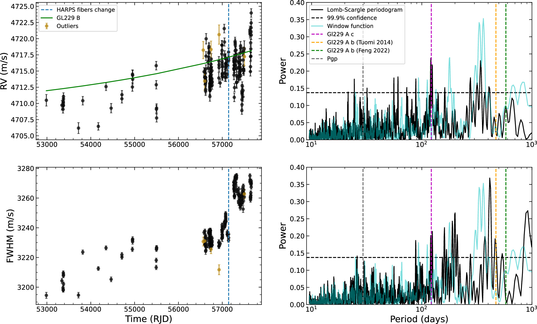
Figure 1. Top left: RV time series with, in green, the G. M. Brandt et al. (2021) orbital solution of Gl 229 B. Bottom left: FWHM time series inferred from the LBL dLW activity indicator. The vertical blue dashed line separates the values obtained before and after the optical fibers change in the HARPS instrument. Data points in yellow are those with an SNR lower than 50. Right panels: Lomb–Scargle periodograms of the RVs (top) and FWHM (bottom). The vertical dashed lines represent the reported period of 121.933 days for planet Gl 229 A c (F. Feng et al. 2022; in pink), the reported period of 471 days for planet Gl 229 A b (M. Tuomi et al. 2014; in yellow), the other reported period for planet Gl 229 A b of 579.474 days (F. Feng et al. 2022; in green), and the rotation period of the star (in gray) at 28.9 days. The horizontal black dashed line represents the 99.9% confidence level. The window function is displayed in cyan.
Download figure:
Standard image High-resolution image3.1. Gl 229 B
Using the orbital parameters shown in Table 1, we calculated the RV signal induced by Gl 229 B on its host with the Radvel Python package (B. J. Fulton et al. 2018). Figure 2 shows this RV signal but on a ∼410 yr span corresponding to almost two full orbits of 86,909 days. The RV variations during the observational baseline of 1000 days is ≈7 m s–1, as shown in the zoomed portion of the figure.
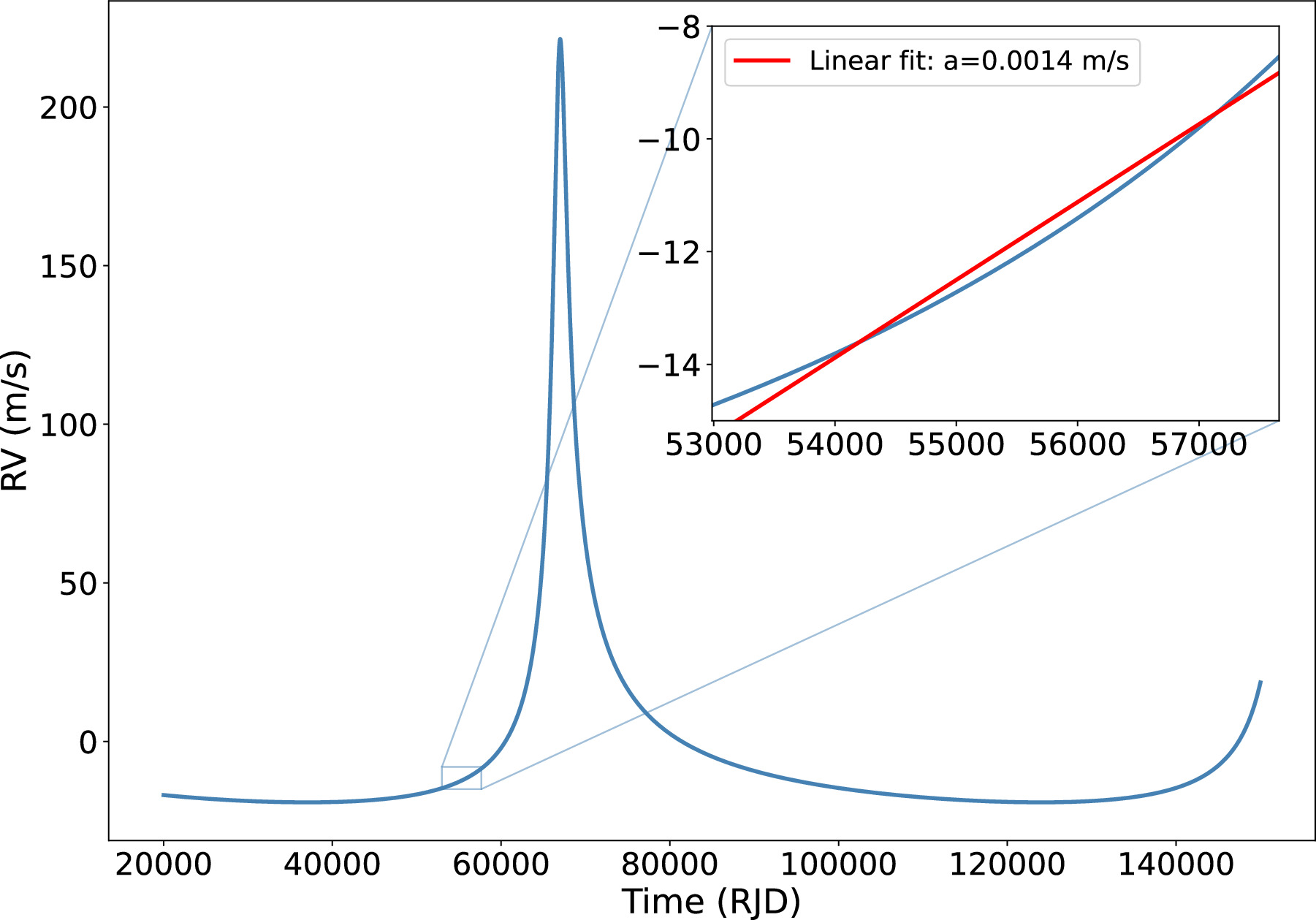
Figure 2. Radial velocity variations of Gl 229 A induced by its BD companion Gl 229 B using the orbital solution from G. M. Brandt et al. (2021). The BD is on an 86,909 days, eccentric (e = 0.851) orbit, inducing a K ≈ 120 m s–1 radial velocity signal. The zoomed-in subpanel displays the RV change during the HARPS measurements time span with, in red, a linear fit.
Download figure:
Standard image High-resolution imageAs shown in Figure 2, the RVs induced by the BD at the epochs of the HARPS observations correspond approximately to a linear function. We did a first estimate to discriminate between linear or higher-order polynomials fit. On the BD's calculated RVs (shown in Figure 2), the slope of the linear function is 0.0014 m s–1 day−1. Higher-order terms did not improved the fit. In Section 3.3, a linear fit is then applied to the HARPS data.
3.2. Stellar Activity Characterization
A Gaussian process (GP) regression with a quasiperiodic covariance function (kernel) was used to model the LBL FWHM time series. In recent years, GP regressions have become the standard for accurate modeling of quasiperiodic variations in astronomical time series (e.g., R. D. Haywood et al. 2014; S. Aigrain et al. 2016; V. Rajpaul et al. 2016). The quasiperiodic kernel used in this work has been shown to efficiently model the quasi-sinusoidal flux variations of a rotating star caused by its different active regions and spot patterns while keeping a reasonable number of nondegenerate parameters (R. D. Haywood et al. 2014; R. Angus et al. 2018).
In an explicit form, the quasiperiodic covariance function is:

where A is the amplitude of the GP, Δt is the time interval between data i and j, ℓ is the exponential timescale, Γ the coherence scale of the correlations, PGP is the period of the GP, and s is an additional white-noise term added in quadrature to the diagonal of ki,j.
Since we aim to model the rotation of the star, non-long-period signals related to the magnetic cycle, only the high-cadence part of the dataset was used. To ensure that the instrumental effects caused by the optical fibers upgrade on HARPS would not bias the stellar activity model, the pre- and postdata were attributed different offsets:  and δpost.
The Python (F. Perez & B. E. Granger 2007) module george (S. Ambikasaran et al. 2015) was used to calculate the Gaussian logarithmic likelihood function and GP predictions. The model hyperparameters consisted of lnA, lnℓ, lnΓ, lnPGP, s,  , and δpost, for which we used the broad, uniform priors given in Table 2. The corresponding posterior distributions were sampled using the Markov chain Monte-Carlo (MCMC) ensemble sampler emcee (D. Foreman-Mackey et al. 2013). 100 walkers were used, running for 20,000 steps, with the first 2000 rejected as burn in. It was ensured that the number of steps was greater than 50 times the autocorrelation timescale calculated by emcee for each parameter to allow sufficient convergence (A. Sokal 1997; D. Foreman-Mackey et al. 2013).
Table 2. Fitted Hyperparameters of the Gaussian Process on the FWHM
| Parameter | Prior | Posterior | Description |
|---|---|---|---|
 [m s–1] [m s–1] |

| 1.697 ± 0.203 | Amplitude of the GP |
 [days] [days] |

| 3.742 ± 0.227 | Exponential timescale of the GP |

|

| −0.664 ± 0.533 | Coherence scale of the correlations |
 [days] [days] |

| 3.363 ± 0.056 | Period of the GP |
 [m s–1] [m s–1] |

| −3234.390 ± 2.195 | FWHM HARPS offset, predata |
| δpost [m s–1] |

| −3264.315 ± 2.484 | FWHM HARPS offset, postdata |
| s [m s–1] |

| 1.702 ± 0.217 | White-noise term |
Note. Units: Γ is dimensionless.
Download table as: ASCIITypeset image
Figure 3 shows the mean prediction of the best-fit GP on the FWHM data. The resulting posterior distributions are shown in Figure B1. Their medians, 16th, and 84th percentiles values are listed in Table 2. We measure a period of 28.9 ± 1.6 days for the GP.
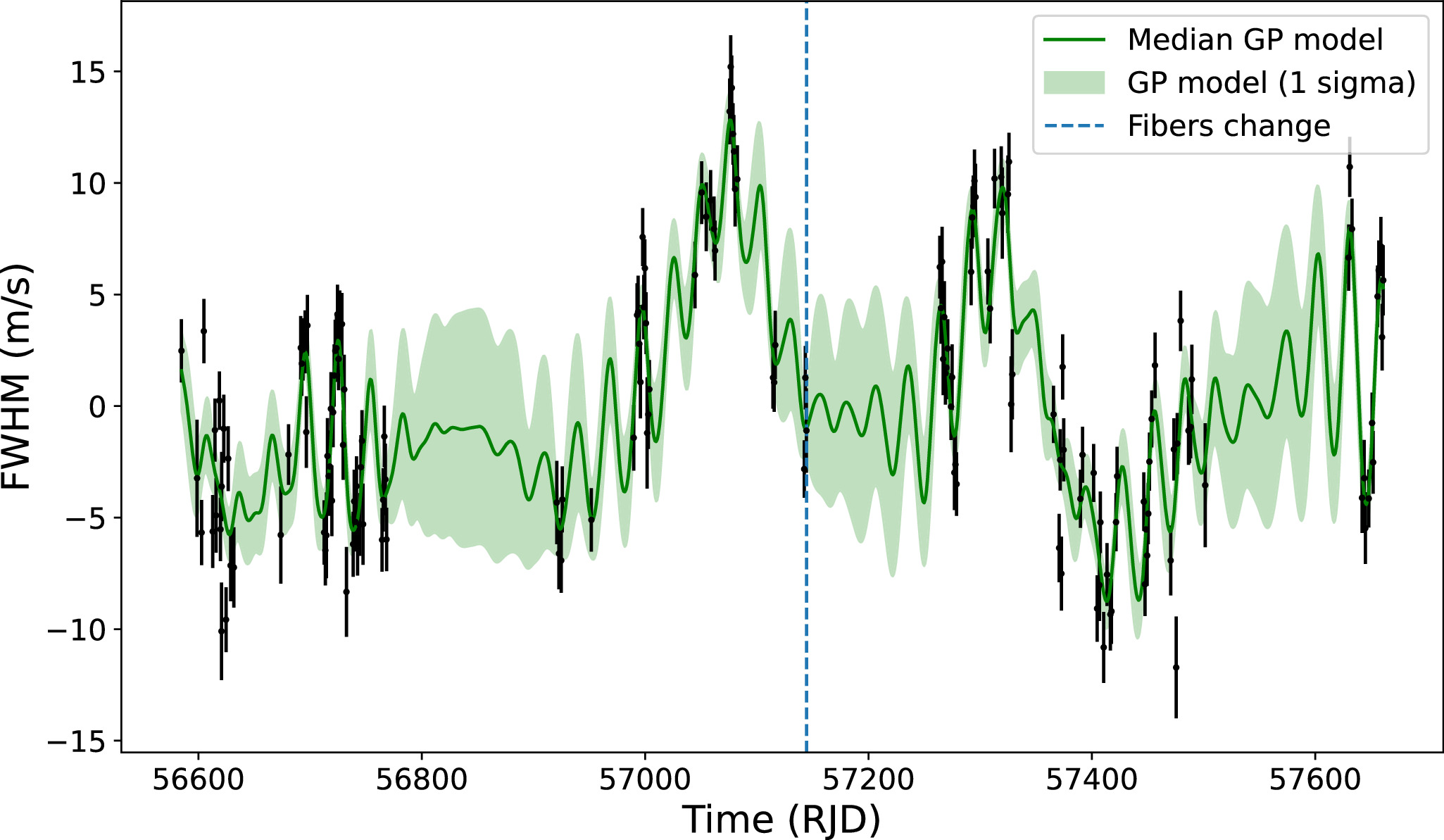
Figure 3. The high-cadence part of the FWHM time series shows the ∼30 days rotation period. The vertical blue dashed line represents the HARPS fiber upgrade. The green curve shows the mean prediction of the best-fit quasiperiodic Gaussian process with its 1σ confidence envelope.
Download figure:
Standard image High-resolution imageThe GP recovers a periodic signal at 28.9 ± 1.6 days, consistent with the measured rotation period of the star (27.3 ± 0.2 days) inferred from photometric time series (E. D. Alonso et al. 2019). Twenty-five days have also been inferred by N. Astudillo-Defru et al. (2017) using the measured chromospheric emission and the correlations between rotation and activity. Our analysis suggests that the peak seen at ∼120 days in the FWHM periodogram (see Figure 1) is most likely an alias of the rotation period as it is close to four times PGP.
3.3. Radial Velocity Analysis
The GP stellar activity model above was used to make a joint model of stellar activity and planetary signals in the RV data. We modeled stellar activity in the HARPS RVs with a quasiperiodic GP where the priors on the hyperparameters are Gaussian distributions following the posteriors of the FWHM fit (see Table 2). Two types of model are considered: Model 1, a stellar activity model and a linear term representing the BD; and Model 2, a joint stellar activity and planetary model (including a linear drift for the BD) with multiple iterations (Model 3 to 5) representing planets with different period priors. The analysis is performed on the full dataset to sample potential long-period planets as previously claimed (e.g., ∼600 days for planet b).
The model includes the RV systemic velocities,  and γpost, to allow for a potential offset following the optical fiber upgrade.
The top part of Table 3 presents the priors and posteriors of Model 1. The GP hyperparameters A, the amplitude, and s, the additional white-noise term, are considered free parameters while the others have Gaussian priors. Similarly to Section 3.2, we sampled the joint posterior distribution with emcee using 100 walkers for 40,000 steps and a 5000 burn in.
Table 3. Fitted Orbital Parameters for Gl 229 A RV's and Activity GP
| Parameter | Prior | Posterior | Description |
|---|---|---|---|
| Model 1: No Planet | |||
| BIC: 867 | |||
| Activity GP Parameters | |||
 [m s–1] [m s–1] |

|

| Amplitude of the GP |
 [days] [days] | (FWHM)a |

| Exponential timescale of the GP |

| (FWHM)a |

| Coherence scale of the correlation |
 [days] [days] | (FWHM)a |

| Period of the GP |
| s [m s–1] |

| 0.91 ± 0.10 | Extra white-noise term |
| Fitted Parameters | |||
 [m s–1] [m s–1] |

| −4715.8 ± 0.8 | RV HARPS offset, predata |
| γpost [m s–1] |

| −4715.4 ± 0.9 | RV HARPS offset, postdata |
| a [m s–1 day−1] |

| 0.0019 ± 0.0004 | Slope of linear term |
| Model 2: One Planet (Uniform Prior on P) | |||
| BIC: 892 | |||
| Activity GP Parameters | |||
 [m s–1] [m s–1] |

|

| Amplitude of the GP |
 [days] [days] | (FWHM)a |

| Exponential timescale of the GP |

| (FWHM)a |

| Coherence scale of the correlation |
 [days] [days] | (FWHM)a |

| Period of the GP |
| s [m s–1] |

| 0.92 ± 0.10 | Extra white-noise term |
| Fitted Parameters | |||
 [m s–1] [m s–1] |

| −4715.8 ± 0.9 | RV HARPS offset, predata |
| γpost [m s–1] |

| −4715.5 ± 0.9 | RV HARPS offset, postdata |
| a [m s–1 days−1] |

| 0.0012 ± 0.0006 | Slope of linear term |
| T0 [RJD] |

| 57238 ± 14 | Time of inferior conjunction |
| P [days] |

|

| Orbital period |
| K [m s–1] |

|

| RV semiamplitude |
| Model 3: One Planet (Gaussian Prior on P, Planet b) | |||
| BIC: 906 | |||
| Fitted Parameters | |||
| P [days] |

|

| Orbital period |
| K [m s–1] |

|

| RV semiamplitude |
| KRef [m s–1] | … |

| Reported semiamplitudeb |
| Model 4: One Planet (Gaussian Prior on P, Planet b) | |||
| BIC: 907 | |||
| Fitted Parameters | |||
| P [days] |

|

| Orbital period |
| K [m s–1] |

|

| RV semiamplitude |
| KRef [m s–1] | … |

| Reported semiamplitudec |
| Model 5: One Planet (Gaussian Prior on P, Planet c) | |||
| BIC: 887 | |||
| Fitted Parameters | |||
| P [days] |

|

| Orbital period |
| K [m s–1] |

|

| RV semiamplitude |
| KRef [m s–1] | … |

| Reported semiamplitudeb |
Notes. Note that for Models 3 to 5, only the period, semiamplitude, and reported semiamplitude are indicated, as these are the only parameters with significant changes between the models. The other parameters remain approximately the same as those in Model 2. aGP(FWHM) is the posterior distribution on the hyperparameter from the FWHM GP, Γ is dimensionless. bF. Feng et al. (2022). cM. Tuomi et al. (2014).
Download table as: ASCIITypeset image
Figure 4 displays, from top to bottom: the RVs, the activity model, the BD linear term, and the residuals while Figure B2 presents the posterior distributions of all parameters.
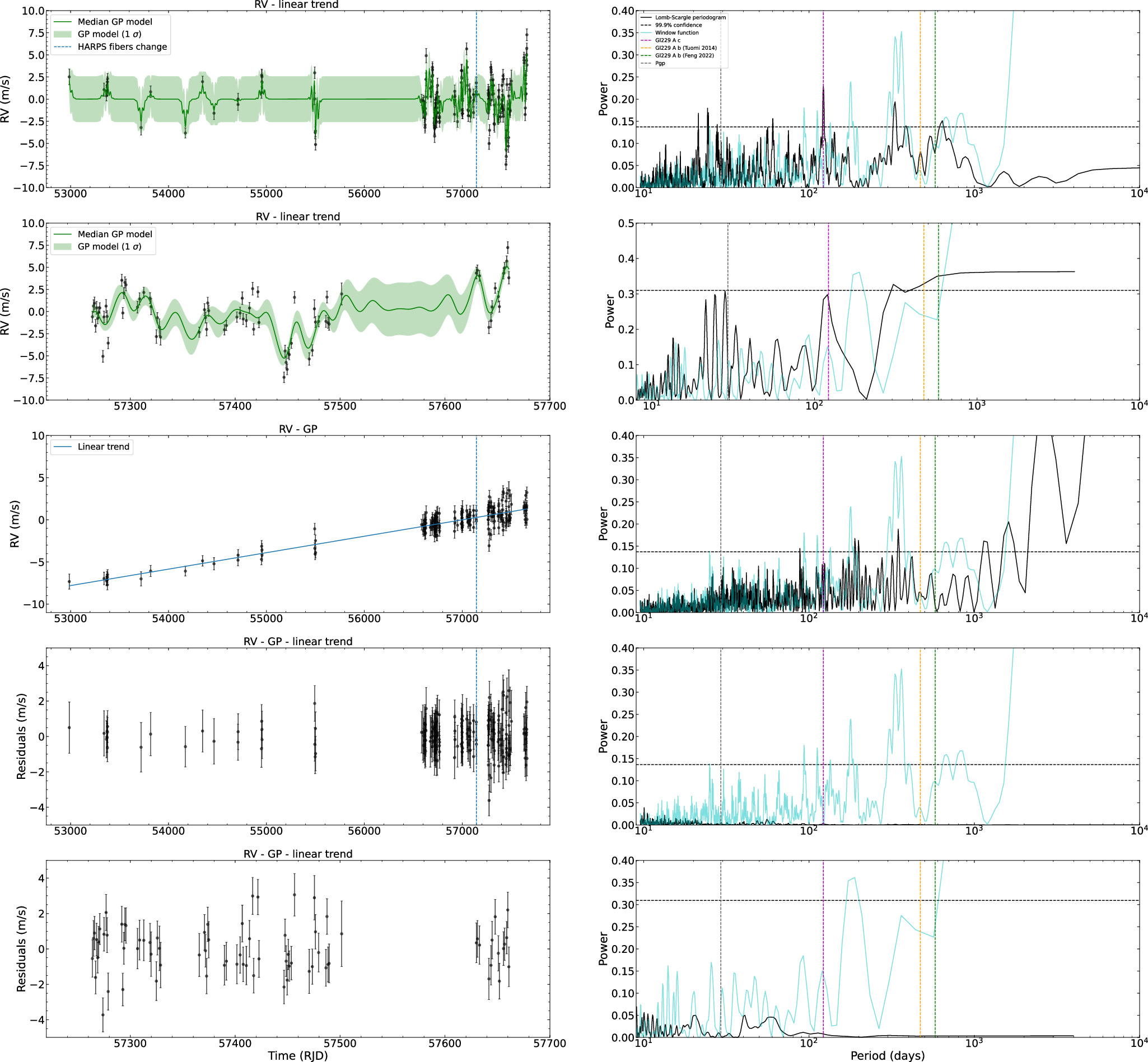
Figure 4. Summary of the RV analysis of Gl 229. Left panels: RV contribution from stellar activity with the mean prediction of the activity model (green curve) with its 1σ confidence envelope, for the full dataset and the postfiber change data. The middle plot represent the linear component to capture the BD effects (blue curve). Following are the residuals of the best-fit joint model (activity + linear trend) for both datasets. The vertical blue dashed line in the first, third, and fourth panels separates the values obtained before and after the optical fibers change in the HARPS instrument. Right panels: the corresponding Lomb–Scargle periodogram (in black) after subtracting the different components of the model and the associated window function (in cyan). Various relevant periodicities are shown with dashed vertical lines (same as in Figure 1).
Download figure:
Standard image High-resolution imageBoth periods attributed to Gl 229 A b (471 ± 22 or 579.47 ± 1.68 days, M. Tuomi et al. 2014; F. Feng et al. 2022) together with the one attributed to Gl 229 A c (121.933 ± 0.082 days) disappear with the stellar activity GP used in Model 1.
During their analysis, F. Feng et al. (2020) mentioned that the signal of Gl 229 A c was more significant in the HARPS postfiber change dataset due to its higher cadence. Model 1 was then also conducted on the postmeasurements exclusively using the same protocol as described above to assess if consistent results were obtained. A summary of this analysis is presented in Figure 4. Our results remain unchanged: the LBL data provide no evidence for planets. The other models (2 to 5) were also tested on the postmeasurement dataset. Since the conclusions drawn were consistent with those from the full dataset, we opted to exclude these results from the text to maintain clarity and conciseness.
We then tested Model 2 to 5 to search for a potential planet in the system. Table 3 presents the priors and posteriors. All parameters describing the Keplerian orbit have large and uniform priors. For Model 2 to 5, we used 100 MCMC walkers, 100,000 steps and a burn in of 10,000 to sample the posterior distribution.
The posteriors did not converge to a well-defined orbital period. When calculating the Bayes Information Criterion (BIC, G. Schwarz 1978), a value of 892 is obtained compared to 867 for Model 1 giving a ΔBIC = 25. The smallest BIC corresponds to the preferred model meaning it is compelling evidence in favor of Model 1. Our analysis suggests that the model with a planet is highly disfavored (R. E. Kass & A. E. Raftery 1995).
The model was also run with a Gaussian prior on the orbital period (P) using the reported values of the claimed planets Gl 229 A b and A c through Model 3 to 5. Planet b has different periods and semiamplitudes published in M. Tuomi et al. (2014) and F. Feng et al. (2022), they were both tested. These planets are not favored by the BIC compared to Model 1, as can be seen in Table 3, the BIC values obtained for Model 3 to 5 are all much higher than the one for Model 1. The semiamplitude of the planet reported by M. Tuomi et al. (2014) is excluded with a 95% confidence level from the K distribution obtained by our model. We also reject a semiamplitude larger than the one obtained in F. Feng et al. (2022) with 92% confidence. As for planet c, we cannot reject the semiamplitude of F. Feng et al. (2022), the model with an informed period has a ΔBIC = 20, strongly preferring the simpler model with no Keplerian.
During our analysis, we identified concerns regarding the potential for GP overfitting with lower cadence data. To investigate this issue, we tested the potential causes of overfitting outlined in Section Four of S. Blunt et al. (2023). First, we addressed the challenge of Correlated Datasets versus Datasets that Share Hyperparameters by allowing distinct amplitudes, white-noise levels, and RV zero points for both the comprehensive dataset and the high-cadence subset. Second, for the Prot and Prot/2 issue, we employed a GP with a single-period parameter instead of the two typically used in the rotational kernel (D. Foreman-Mackey 2018), which could be fit for this analysis. This approach reduces the number of parameters to fit, thereby decreasing the risk of overfitting. Third, regarding the concern that Keplerian Parameters Enable Overfitting in the Presence of Unmodeled Noise, we tested the GP both without Keplerian components and with one or two planets. Finally, for the issue of Differential Rotation, we applied our model to high-cadence data derived from the post-HARPS fiber change dataset.
4. Discussion
4.1. Stellar Activity False Positive
Our results emphasize the importance of adequately modeling stellar activity as it can be mistaken for genuine Keplerian signals. Stellar activity is particularly acute for M dwarfs characterized by deep convection zones (C. A. Ortiz-Rodrguez et al. 2022) that generate active regions, spots, and faculae, affecting a significant fraction of their surface (J. R. Barnes et al. 2011). These active regions produce asymmetries in the shape of the spectral lines inducing an RV shift (S. V. Jeffers et al. 2022), which can be mistaken as a planetary signal.
Gl 229 is adding to a growing list of M-dwarf systems in which stellar activity was mistaken as planets, e.g., the formerly identified HZ planets in GL581 (P. Robertson et al. 2014) and GJ832 (P. Gorrini et al. 2022). Our work and recent others call for a reanalysis of existing RV data for M dwarfs. There is a sizable sample of 141 RV planets orbiting such stars, of which 36 have relatively long orbital periods between 30 and 700 days (R. L. Akeson et al. 2013). Long-period, low-RV amplitude planets are particularly prone to systematics effects, e.g., the long-period planets Proxima c (M. Damasso et al. 2020) and Gl 699 b (I. Ribas et al. 2018) now demonstrated to be artifacts (J. Lubin et al. 2021) even through an LBL analysis (E. Artigau et al. 2022). Identifying these false positive planets is essential as they bias occurrence rates and our understanding of exoplanet demographics. They also misguide follow-up observing programs.
4.2. Mass Limit for a Planet in the Habitable Zone
The formation of planets in binary systems with separations smaller than 50–100 au is believed to be highly challenging. Observational evidence suggests that binary companions on such separation scales prevent the formation or survival of planets, with fewer planets observed around such systems compared to longer-period binaries (C. Bergfors et al. 2013; A. L. Kraus et al. 2016; M. Bonavita & S. Desidera 2020). Similarly, very few close-in binary companions are seen among the sample of known exoplanets (C. Fontanive et al. 2019; C. Fontanive & D. Bardalez Gagliuffi 2021), despite such binaries being the most common in the stellar field population (separation distribution peaking around 50 au for Sun-like stars; D. Raghavan et al. 2010). Studies of binaries at young ages have also revealed lower circumstellar disk fractions and shorter disk lifetimes in binaries below about 100 au separations (A. L. Kraus & M. J. Ireland 2012), both unfavorable effects to planet formation. Due to the many biases against binaries and incompleteness in existing data (C. Fontanive & D. Bardalez Gagliuffi 2021), the boundaries from which the effects of binary companions become detrimental to the formation or survival of close-in planets are not clear. In particular, the minimum separation from which companions might influence inner planetary systems is likely to shift with companion mass (e.g., J. Cadman et al. 2022). Existing data for systems like Gl 229, with a BD as a binary companion, are currently insufficient to draw robust conclusions on how observed trends in the stellar regime might extend to substellar companions. Nonetheless, with a mass close to the BD/star boundary and a semimajor axis of only 33 au, the presence of GL 229 B would be hard to reconcile with the existence of two small planets around the primary star. Although more extreme systems (smaller than 20 au) are known to exist (D. Queloz et al. 2000; A. P. Hatzes et al. 2003), these exceptions mostly seem to be massive, close-in giant planets, which exhibit somewhat different demographics for the population of such planets in binaries (C. Fontanive & D. Bardalez Gagliuffi 2021), possibly linked to a different gravitational-instability origin of the planets themselves (J. Cadman et al. 2022). As the planets around GL 229 would be much smaller, their existence would remain in tension with our understanding of planet formation in binaries given the presence of the nearby and massive GL 229 B BD companion.
Given the existing RV dataset, one can set an upper mass limit on a possible planetary companion orbiting the HZ of Gl 229 A. The HZ ranges from ∼24 to ∼97 days according to Equation (5) of R. K. Kopparapu et al. (2014) using the coefficient for the recent Venus/early Mars limits. The period corresponding to the same flux received by Earth is ∼43 days.
The RVs induced by planets of different semiamplitudes were generated for the whole dataset with the function rv_drive() from the radvel module (B. J. Fulton et al. 2018) for various periods. The first one, around ten days, is the minimal period detectable with the sampling of our dataset as the window function does not exhibit any signal before this period. A circular orbit was assumed for all cases.
RV's of the simulated planets were added into the data with white noise and then retrieved running Model 2, meaning a stellar activity model with a Keplerian model for one planet. The priors used were the same as for Model 2. We define a planet as detected when it is retrieved with a confidence level greater than 3σ on the retrieved semiamplitude.
Figure 5 summarizes the results, showing the 3σ upper limit as a function of the orbital period; the shaded area represents the HZ.
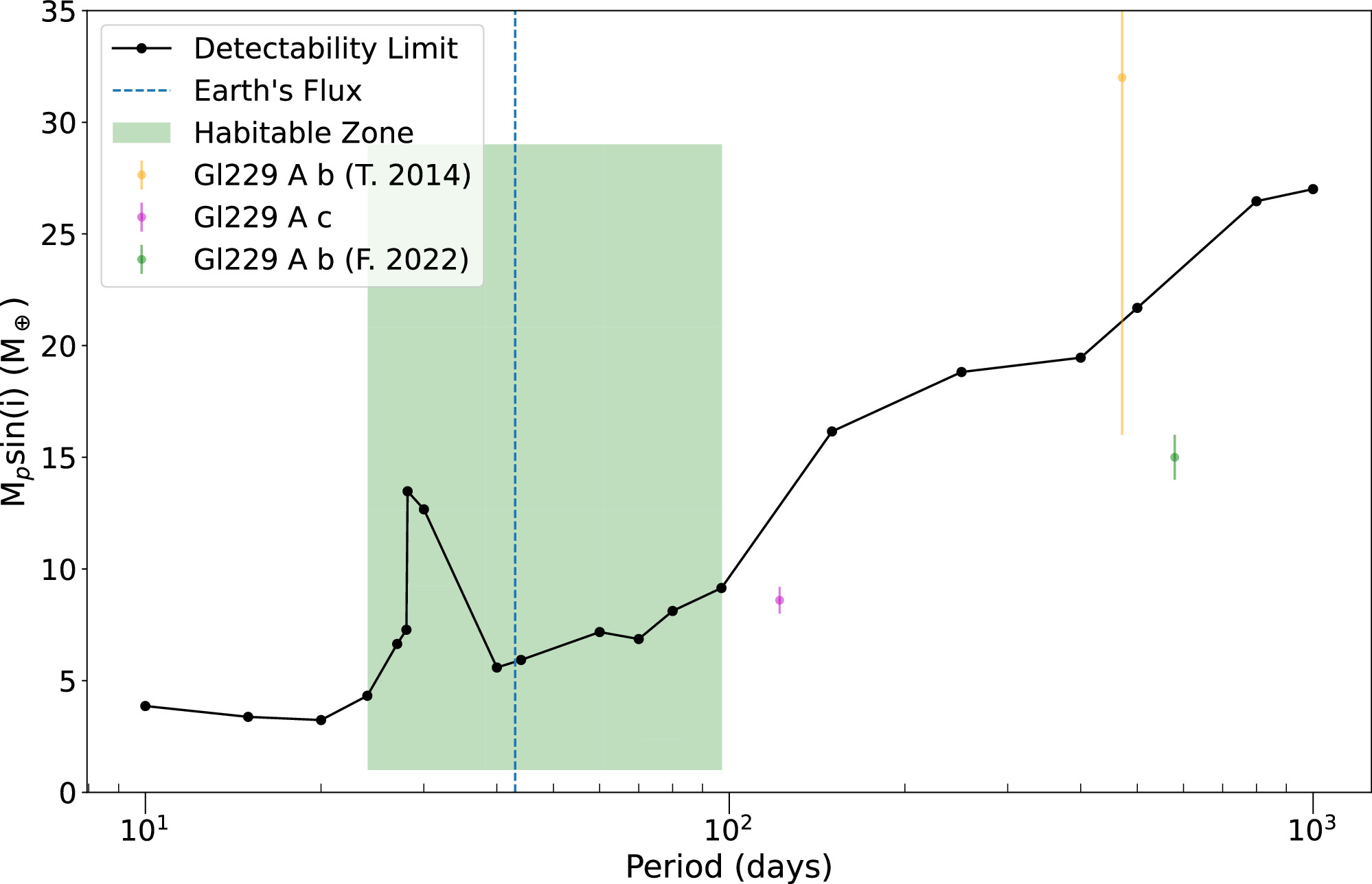
Figure 5. Detection limit for a planet in the Gl 229 system. The black line represents the minimal  at which a planet can be detected at the associated period with the LBL dataset. The tested periods are represented by the black dots. The green-shaded region delimits the system's HZ, while the vertical blue dashed line indicates the orbital period at which the received flux is the same as Earth. The previously claimed planet Gl 229 A b and c are also represented by dots, respectively in orange, green, and pink.
Download figure:
Standard image High-resolution imageThis analysis sets mass upper limits of 4.3 and 9.1 M⊕ for the inner and outer edge of the HZ, respectively. This limit is higher, around 12.7 M⊕, at the periods close to the star's rotation period. At the exact rotation period, 28.9 days, it is very difficult to retrieve a planet, as it is removed by the activity model. Planet b and c were most recently reported as having a minimal mass of ∼15M⊕ and ∼8.6 M⊕ (F. Feng et al. 2022). We thus cannot exclude with 99.7% confidence planets of such masses at orbital periods greater than ∼100 days. This upper limit corresponds to a blind search using uniform priors on orbital periods and phase in contrast with our test in Section 3.2 where we forced the orbital period to be close to the claimed planets. Furthermore, the RV signal around 120 days are also close to the rotation period aliases. As a result, the activity GP model tends to remove planets injected at these periods, increasing their detectability limit.
5. Conclusion
We have presented a reanalysis of the HARPS RVs for the Gl 229 system. We used the LBL method to extract the RV measurements and FWHM variations from the publicly available spectra. We produced a stellar activity model from which we infer a rotation period of 28.9 ± 1.6 days for Gl 229 A.
The analysis shows that the Keplerian signals previously attributed to planets Gl 229 A b and Gl 229 A c (M. Tuomi et al. 2014; F. Feng et al. 2020) with orbital periods of ∼122, ∼471, and ∼579 days vanish when stellar activity is taken into account. Therefore, we can exclude at the 3σ level the presence of a planet with a mass higher than 9.1 M⊕ in the system's HZ except at periods close to the rotation of the star.
Acknowledgments
Based on data obtained from the ESO Science Archive Facility. This work was possible thanks to the financial support of the Natural Science and Engineering Research Council of Canada and the Trottier Family Foundation in their support of IREx.
Facilities: European Southern Observatory (ESO) 3.6m Telescope at La Silla Observatory - .
Software: Astropy (The Astropy Collaboration et al. 2013), matplotlib (J. D. Hunter 2007), NumPy (C. R. Harris et al. 2020), george (S. Ambikasaran et al. 2015), corner (D. Foreman-Mackey 2016), emcee (D. Foreman-Mackey et al. 2013), radvel (B. J. Fulton et al. 2018).
Appendix A: Data
The complete set of Gl 229 data obtained with the LBL method and shown in Figures 1, 3, and 4 is available in a machine-readable format in the online Journal. Table A1 provides a sample of the values provided.
Table A1. Gl 229 Data Obtained with the LBL Method
| Time | FWHM | σFWHM | RV | σRV |
|---|---|---|---|---|
| (RJD) | (m s–1) | (m s–1) | (m s–1) | (m s–1) |
| 52986.75 | 3194.51 | 2.01 | 4710.48 | 0.89 |
| 53341.82 | 3204.32 | 1.66 | 4709.73 | 0.74 |
| 53366.74 | 3199.51 | 1.28 | 4709.08 | 0.57 |
| 53370.74 | 3198.19 | 1.37 | 4709.67 | 0.61 |
| 53372.70 | 3198.10 | 1.45 | 4710.27 | 0.65 |
Only a portion of this table is shown here to demonstrate its form and content. A machine-readable version of the full table is available.
Download table as: Machine-readable (MRT)Typeset image
Appendix B: Corner Plots
Figures B1 and B2 show the posterior distributions of the best-fit GP on the FWHM data and RV data, respectively.
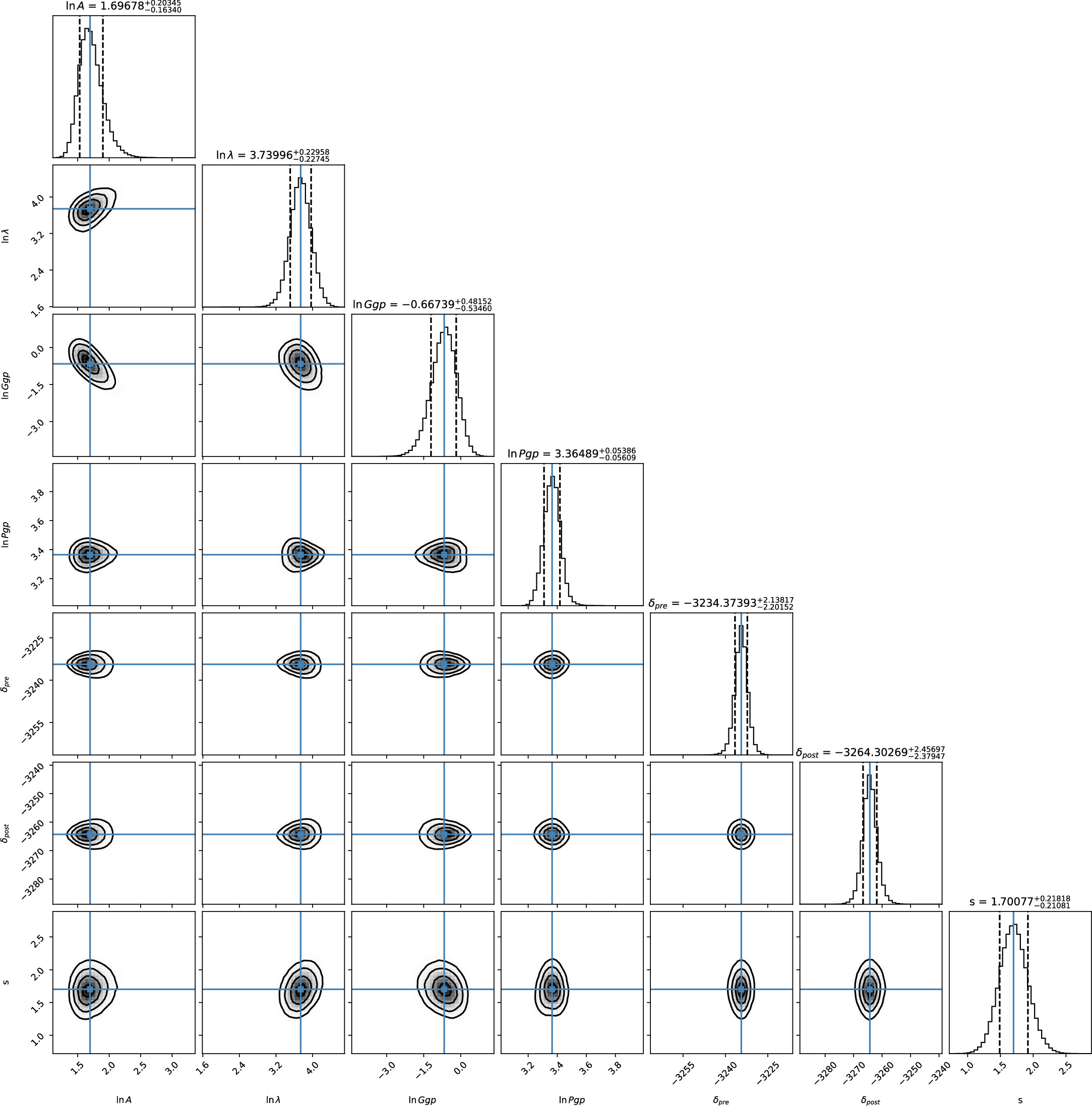
Figure B1. Posterior distributions of the activity model parameters. Contours denote the 1σ, 2σ, and 3σ confidence level. The blue lines indicate the median of the distributions, and the vertical black dashed lines represent the 16th and 84th percentiles.
Download figure:
Standard image High-resolution image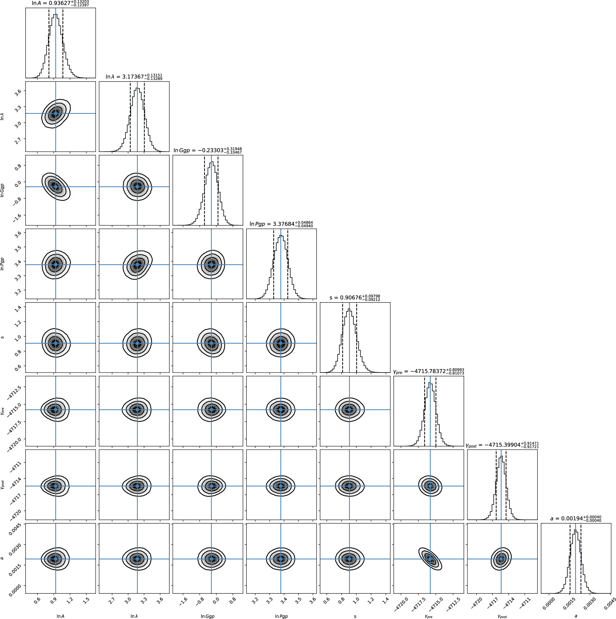
Figure B2. Posterior distributions of Model 1 parameters. Contours denote the 1σ, 2σ, and 3σ confidence level. The blue lines indicate the median of the distributions, and the vertical black dashed lines represent the 16th and 84th percentiles.
Download figure:
Standard image High-resolution image