Abstract
Two narrow and dense rings (called C1R and C2R) were discovered around the Centaur object (10199) Chariklo during a stellar occultation observed on 2013 June 3. Following this discovery, we planned observations of several occultations by Chariklo’s system in order to better characterize the physical properties of the ring and main body. Here, we use 12 successful occulations by Chariklo observed between 2014 and 2016. They provide ring profiles (physical width, opacity, edge structure) and constraints on the radii and pole position. Our new observations are currently consistent with the circular ring solution and pole position, to within the ±3.3 km formal uncertainty for the ring radii derived by Braga-Ribas et al. The six resolved C1R profiles reveal significant width variations from ∼5 to 7.5 km. The width of the fainter ring C2R is less constrained, and may vary between 0.1 and 1 km. The inner and outer edges of C1R are consistent with infinitely sharp boundaries, with typical upper limits of one kilometer for the transition zone between the ring and empty space. No constraint on the sharpness of C2R’s edges is available. A  upper limit of ∼20 m is derived for the equivalent width of narrow (physical width
  km) rings up to distances of 12,000 km, counted in the ring plane.
1. Introduction
The asteroid-like body (10199) Chariklo is a Centaur object orbiting between Saturn and Uranus. It probably moved recently (∼10 Myr ago) from the trans-Neptunian region to its present location and will leave it within a similarly short timescale, due to perturbations by Uranus (Horner et al. 2004). With a radius of 119 ± 5 km, estimated from thermal measurements (Fornasier et al. 2014), it is the largest Centaur known to date, but still remains very modest in size compared to the telluric or giant planets. On 2013 June 3, a ring system was discovered around this small object during a stellar occultation. Two dense and narrow rings, 2013C1R and 2013C2R (C1R and C2R for short), were detected. They are separated by about 15 km and orbit close to 400 km from Chariklo’s center (see Braga-Ribas et al. 2014 for details).
Until 2013, rings were only known around the giant planets. This discovery was thus surprising, and is key to better understanding the planetary rings, since they now appear to be more common than previously thought. In particular, the two rings, being dense, narrow, and (at least for C1R) sharp-edged, look like several of the dense ringlets seen around Saturn and Uranus (Elliot et al. 1984; French et al. 1991, 2016). In that context, there was a strong incentive for planning more occultation campaigns, first to unambiguously confirm the existence of Chariklo’s rings and second, to obtain more information on their physical properties.
While the discovery occultation of 2013 June 3 provided the general physical parameters of the rings (width, orientation, orbital radius, optical depth, …), several questions are still pending, some of which are addressed in this work: Do the rings have inner structures that give clues about collisional processes? How sharp are their edges? What are the general shapes of C1R and C2R? Do they consist of solidly precessing ellipses like some of Saturn’s or Uranus’ ringlets? Do they have more complex proper modes with higher azimuthal wave numbers? Are there other fainter rings around Chariklo? What is the shape of the object itself and its role in the ring dynamics? Based on new results, what can we learn about their origin and evolution, which remain elusive (Sicardy et al. 2016)?
This study is made in the context where material has also been detected around the second largest Centaur, Chiron (again using stellar occultations). The nature of this material is still debated, and it could be interpreted as either a ring system (Ortiz et al. 2015) or a dust shell associated with Chiron’s cometary activity (Ruprecht et al. 2015). Since Chariklo is presently moving close to the galactic plane, stellar occultations by this body are much more frequent than for Chiron; hence, we have more abundant information about its rings. The spatial resolution achieved during occultations reaches the sub-kilometer level, which is impossible to attain with any of the current classical imaging instruments. That said, the very small angular size subtended by the rings (0.08 arcsec tip to tip, as seen from Earth) has made occultation predictions difficult in the pre-Gaia era.
In spite of these difficulties, we were able to observe 13 positive stellar occultations (including the discovery one) between 2013 and 2016, from a total of 42 stations distributed worldwide (in Brazil, Argentina, Australia, Chile, La Réunion Island, Namibia, New Zealand, South Africa, Spain, Thailand, and Uruguay). Here, we focus on the ring detections (a total of 11 chords recorded after the discovery). We also obtained a total of 12 occultation chords by the main body from 2014 to 2016. Their timings are derived here, but their implications concerning Chariklo’s size and shape will be presented elsewhere (Leiva et al. 2017). In Section 2, we present our observations and data analysis. In Section 3, we concentrate on the rings structures (width, inner structures, edge sharpness) and geometry (radius and orbital pole). The integral properties of the rings (equivalent width and depth) are derived in Section 4, before concluding remarks are given in Section 5.
2. Observations and Data Analysis
Following the ring discovery of 2013 June 3, we predicted and observed 12 positive stellar occultations by Chariklo and/or its rings between 2014 and 2016. In the following list, we mark in italic the events that led to multichord ring detections (thus providing constraints on the ring orientation, as discussed latter). Four occultations were observed on 2014 February 16 (rings), March 16 (rings), April 29 (rings and body), and June 28 (rings and body). In 2015, only two positive detections were recorded, April 26 (rings) and May 12 (body), while six occultations were recorded in 2016, July 25 (body), August 8 (rings and body), August 10 near 14 hr UT (body), August 10 near 16 hr UT (body), August 15 (body), and October 1 (rings and body).
2.1. Predictions
Predicting stellar occultations by Chariklo and its rings is a difficult task, as the main body subtends about 25 milliarcsec (mas) as seen from Earth, while the rings have a span of about 80 mas. Thus, to be effective, predictions require accuracies of a few tens of milliarcseconds on both Chariklo’s ephemeris and the star position. To meet this requirement, we used a bootstrapping approach, in which each new detection of an occultation is used to improve Chariklo’s ephemeris, thus providing a better prediction for the next occultation. This continuous update results in the so-called NIMA (Numerical Integration of the Motion of an Asteroid; Desmars et al. 2015) ephemeris accessible online.55
The candidate stars for events in 2014 and in 2016 were identified during a systematic search for occultations by TNOs using the Wide Field Imager (WFI) at the ESO/MPG 2.2 m telescope (Camargo et al. 2014), with typical accuracies of ∼30 mas. However, for the 2015 season, the candidate stars were observed using only the IAG 0.6 m telescope at OPD/LNA in Brazil, which has a lower accuracy than WFI, resulting in a larger number of missed events (two successes out of six attempts). In the majority of the cases, the occulted star was imaged a few days or weeks prior to the event in order to improve the astrometry. If possible, the observations were made when Chariklo and the star were in the same field of view in order to cancel out systematic errors. In those cases, the accuracy of the predictions was estimated down to ∼20 mas.
The last occultation in our list (2016 October 1) is special as its prediction was based on the new Gaia DR1 catalog released on 2016 September 15 (Gaia Collaboration et al. 2016). However, the J2000 DR1 star position  ,
,  (at epoch 2015.0) does not account for proper motion. We estimated the latter by using the UCAC4 star position (under the name UCAC4 285-174081) at epoch 2000 and obtained proper motions in right ascension (not weighted by
  ) and declination of
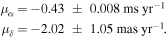
This provides a star position of  ,
,  at the epoch of occultation. Combining this result with the NIMA ephemeris (version 9) finally provided a prediction that agreed to within 5 mas perpendicular to the shadow track and 20 s in terms of timing, and led to a multichord ring and body detection.
2.2. Observations
The circumstances of the observations (telescope, camera, setup, observers, site coordinates, star information) that lead to ring or main body detections are listed in Table 1. Conversely, the circumstances of negative observations (no event observed) are provided in Table 2. Note that observations were made with both small portable telescopes and larger, fixed instruments. Each detection will be designated herein by the name of the station or by the name of the telescope, if well known.
Table 1. Circumstances of Positive Detections (Main Body and/or Rings)
| Date | |||||
|---|---|---|---|---|---|
Rmag(NOMAD catalog),  star coordinates, star coordinates,  stellar diametera stellar diametera
|
|||||
 derived Chariklo’s geocentric coordinates at specified date derived Chariklo’s geocentric coordinates at specified date |
|||||
| Site | Longitude | Telescope | Instrument | Observers | Results |
| Latitude | Exposure Time (s) | ||||
| Altitude (m) | |||||
| 2013 Jun 3 | |||||
R = 12.070,  , ,  , ,  km km |
|||||
at 06:25:30 UT:  , , 
|
|||||
| See details in Braga-Ribas et al. (2014) | |||||
| 2014 Feb 16 | |||||
R = 15.980,  , ,  , ,  km km |
|||||
at 07:45:35 UT:  , , 
|
|||||
| Paranal | 24 37 31. S | UT4 8.2 m | HAWK-I | F. Selman, C. Herrera | C1R and C2R |
| Chile | 70 24 07.95 W | H-filter | 0.25 | G. Carraro, S. Brillant | Partially |
| 2635.43 | C. Dumas, V. D. Ivanov | Resolved | |||
| San Pedro Atacama | 22 57 12.3 S | 50 cm | APOGEE U42 | A. Maury | Main body |
| Chile | 68 10 47.6 W | 10 | N. Morales | ||
| 2397 | |||||
| 2014 Mar 16 | |||||
R = 15.45,  , ,  , ,  km km |
|||||
at 20:31:45 UT:  , , 
|
|||||
| Doi Inthanon | 18 34 25.41 N | TNT 2.4 m | ULTRASPEC | P. Irawati | C1R and C2R |
| Thailand | 98 28 56.06 E | R’-filter | 3.3 | A. Richichi | Unresolved |
| 2450 | |||||
| 2014 Apr 29 | |||||
 , ,  , ,  , ,  kmb kmb
|
|||||
at 23:14:12 UT:  , , 
|
|||||
| SAAO | 32 22 46.0 S | 1.9 m | SHOC | H. Breytenbach | C1R and C2R |
| Sutherland | 20 48 38.5 E | 0.0334 | A. A. Sickafoose | Resolved | |
| South Africa | 1760 | Main body | |||
| Gifberg | 31 48 34.6 S | 30 cm | Raptor Merlin 127 | J.-L. Dauvergne | Grazing C2R |
| South Africa | 18 47 0.978 E | 0.047 | P. Schoenau | ||
| 338 | |||||
| Springbok | 29 39 40.2 S | 30 cm | Raptor Merlin 127 | F. Colas | C1R and C2R |
| South Africa | 17 52 58.8 W | 0.06 | C. de Witt | Sharp and resolved | |
| 900 | |||||
| 2014 Jun 28 | |||||
R = 13.65,  , ,  , ,  km km |
|||||
at 22:24:35 UT:  , , 
|
|||||
| Hakos | 23 14 11 S | 50 cm AK3 | Raptor Merlin 127 | K.-L. Bath | C1R and C2R |
| Namibia | 16 21 41.5 E | 0.2 | Unresolved | ||
| 1825 | |||||
| Kalahari | 26 46 26.91 S | 30 cm | Raptor Merlin 127 | L. Maquet | Main body |
| South Africa | 20 37 54.258 E | 0.4 | |||
| 861 | |||||
| Twee Rivieren | 26 28 14.106 S | 30 cm | Raptor Merlin 127 | J.-L. Dauvergne | Main body |
| South Africa | 20 36 41.694 E | 0.4 | |||
| 883 | |||||
| 2015 Apr 26 | |||||
R = 12.04,  , ,  , ,  km km |
|||||
at 02:11:58 UT:  , , 
|
|||||
| Los Molinos | 34 45 19.3 S | OALM | FLI CCD | S. Roland | CR and C2R |
| Uruguay | 56 11 24.6 W | 46 cm | 0.8 | R. Salvo | Unresolved |
| 130 | G. Tancredi | ||||
| 2015 May 12 | |||||
R = 15.93,  , ,  , ,  km km |
|||||
at 17:55:40 UT:  , , 
|
|||||
| Samford Valley | 27 22 07.00 S | 35 cm | G-star | J. Bradshaw | Main Body |
| Australia | 152 50 53.00 E | 0.32 | Emersion of unresolved | ||
| 80 | rings only | ||||
| 2016 Jul 25 | |||||
R = 14.02,  , ,  , ,  km km |
|||||
at 23:59:00 UT:  , , 
|
|||||
| Liverpool Telescope | 28 45 44.8 N | 2 m | RISE | J.-L. Ortiz | Main Body |
| Canary Islands | 17 52 45.2 W | 0.6 | N. Morales | ||
| 2363 | |||||
| 2016 Aug 08 | |||||
R = 13.67,  , ,  , ,  km km |
|||||
at 19:57:00 UT:  , , 
|
|||||
or  , , 
|
|||||
| Windhoek(CHMO) | 22 41 54.5 S | 35 cm | ZWO/ASI120MM | H.-J. Bode | Main Body |
| Namibia | 17 06 32.0 E | 1 | C1R and C2R | ||
| 1920 | unresolved | ||||
| 2016 Aug 10 | |||||
R = 16.53,  , ,  , ,  km km |
|||||
at 14:23:00 UT:  , , 
|
|||||
| Murrumbateran | 34 57 31.50 S | 40 cm | WATEC 910BD | D. Herald | Main Body |
| Australia | 148 59 54.80 E | 0.64 | |||
| 594 | |||||
| 2016 Aug 10 | |||||
R = 16.22,  , ,  , ,  km km |
|||||
at 16:43:00 UT:  , , 
|
|||||
| Les Makes | 21 11 57.4 S | 60 cm | Raptor Merlin 127 | F. Vachier | Main Body |
| La Réunion | 55 24 34.5 E | 2 | |||
| 972 | |||||
| 2016 Aug 15 | |||||
R = 14.64,  , ,  , ,  km km |
|||||
at 11:38:00 UT:  , , 
|
|||||
| Darfield | 43 28 52.90 S | 25 cm | WATEC 910BD | B. Loader | Main Body |
| New Zealand | 172 06 24.40 E | 2.56 | |||
| 210 | |||||
| 2016 Oct 1 | |||||
R = 15.36,  , ,  , ,  km km |
|||||
at 10:10:00 UT:  , , 
|
|||||
| Rockhampton | 23 16 09.00 S | 30 cm | WATEC 910BD | S. Kerr | Main Body |
| Australia | 150 30 00 E | 0.320 | C1R and C2R | ||
| 50 | unresolved | ||||
| Adelaide | 34 48 44.701 S | 30 cm | QHY 5L11 | A. Cool | Main body |
| Heights School | 138 40 56.899 E | 1 | B. Lade | C1R and C2R | |
| Australia | 167 | Unresolved | |||
Note.
aProjected at Chariklo’s distance (using van Belle 1999, except for 2014 April 29; see the text for details). bThe index A refers to the primary of the binary star.Table 2. Circumstances of Observations that Detected No Event or During Which No Data Were Acquired
| Site | Longitude | Telescope | Instrument | Observers |
|---|---|---|---|---|
| Latitude | Exposure Time (s) | |||
| Altitude (m) | ||||
| 2014 Feb 16 | ||||
| Cerro Tololo | 30 10 03.36 S | 0.4 m | PROMPT | J. Pollock |
| Chile | 70 48 19.01 W | 4 telescopes | 6.0/2.0 | |
| 2207 | ||||
| La Silla | 29 15 16.59 S | TRAPPIST | FLI PL3041-BB | E. Jehin |
| Chile | 70 44 21.82 W | 60 cm | 4.5 | |
| 2315 | ||||
| La Silla | 29 15 32.1 S | NTT 3.55 m | SOFI | L. Monaco |
| Chile | 70 44 01.5 W | H-filter | 0.05 | + visitor team |
| 2375 | ||||
| 2014 Apr 29 | ||||
| Hakos | 23 14 50.4 S | 50 cm AK3 | Raptor Merlin 127 | K.-L. Bath |
| Namibia | 16 21 41.5 E | 0.075 | ||
| 1825 | ||||
| Hakos | 23 14 50.4 S | 50 cm RC50 | i-Nova | R. Prager |
| Namibia | 16 21 41.5 E | 1.0 | ||
| 1825 | ||||
| Windhoek (CHMO) | 22 41 54.5 S | 35 cm | Raptor Merlin 127 | W. Beisker |
| Namibia | 17 06 32.0 E | 0.1 | ||
| 1920 | ||||
| 2014 Jun 28 | ||||
| Les Makes | 21 11 57.4 S | 60 cm | WATEC 910HX | A. Peyrot |
| La Réunion | 55 24 34.5 E | 0.4 | J-P. Teng | |
| 972 | ||||
| 2015 Apr 26 | ||||
| Bigand | 33 26 11 S | 15 cm | Canon Ti | S. Bilios |
| Provincia Santa Fé | 61 08 24 W | 5 | ||
| Argentina | 90 | |||
| Bigand | 33 26 11 S | 15 cm | Canon EOS | J. Nardon |
| Provincia Santa Fé | 61 08 24 W | 3.2 | ||
| Argentina | 90 | |||
| La Silla | 29 15 16.6 S | TRAPPIST | FLI PL3041-BB | E. Jehin |
| Chile | 70 44 21.8 W | 60 cm | 4.5 | |
| 2315 | ||||
| Bosque Alegre | 31 35 54.0 S | 76 cm | QHY6 | R. Melia |
| Argentina | 64 32 58.7 W | 1.2 | C. Colazo | |
| 1250 | ||||
| Santa Rosa | 36 38 16 S | 20 cm | Meade DSI-I | J. Spagnotto |
| Argentina | 64 19 28 W | 3 | ||
| 182 | ||||
| Santa Martina | 33 16 09.0 S | 40 cm | Raptor Merlin 127 | R. Leiva |
| Chile | 70 32 04.0 W | 0.5 | ||
| 1450 | ||||
| Buenos Aires (AAAA) | 34 36 16.94 S | 25 cm | ST9e | A. Blain |
| Argentina | 58 26 04.37 W | 4 | ||
| 0 | ||||
| 2015 May 12 | ||||
| Reedy Creek | 28 06 30.4 S | 25 cm | WATEC 120N+ | J. Broughton |
| Australia | 153 23 52.90 E | 0.64 | ||
| 66 | ||||
| 2016 Jul 25 | ||||
| Granada | 37 00 38.49 N | 60 cm | Raptor Merlin 127 | S. Alonso |
| Spain | 03 42 51.39 W | 0.4 | A. Román | |
| 1043 | ||||
| Albox | 37 24 20.0 N | 40 cm | Atik 314L+ | J.-L. Maestre |
| Spain | 02 09 6.5 E | 3 | ||
| 493 | ||||
| 2016 Aug 10-14 hr UT | ||||
| Blue Mountains | 33 39 51.9 S | 30 cm | WATEC 910BD | D. Gault |
| Australia | 150 38 27.9 E | 5.12 | ||
| 286 | ||||
| Samford Valley | 27 22 07.00 S | 35 cm | WATEC 910BD | J. Bradshaw |
| Australia | 152 50 53.00 E | 0.64 | ||
| 80 | ||||
| Rockhampton | 23 16 09.00 S | 30 cm | WATEC 910BD | S. Kerr |
| Australia | 150 30 00.00 E | 1.28 | ||
| 50 | ||||
| Dunedin | 45 52 20.83 S | 36 cm | Raptor Merlin 127 | F. Colas |
| New Zealand | 170 29 29.90 E | 2. | A. Pennell | |
| 154 | P.-D. Jaquiery | |||
| Sydney | 33 48 35.04 S | 36 cm | Raptor Merlin 127 | H. Pavlov |
| Australia | 150 46 36.90 E | 2.2 | ||
| 37 | ||||
| 2016 Aug 15 | ||||
| Canberra | 35 11 55.30 S | 40 cm | WATEC 910BD | J. Newman |
| Australia | 149 02 57.50 E | 2.56 | ||
| 610 | ||||
| Murrumbateran | 34 57 31.50 S | 40 cm | WATEC 920BD | D. Herald |
| Australia | 148 59 54.80 E | 0.32 | ||
| 594 | ||||
| Greenhill Observatory | 42 25 51.8 S | 1.3 m | Raptor Merlin 127 | K. Hill |
| Tasmania | 147 17 15.8 E | 0.5 | A. Cole | |
| 641 | ||||
| Rockhampton | 23 16 09.00 S | 30 cm | WATEC 910BD | S. Kerr |
| Australia | 150 30 00.00 E | 1.28 | ||
| 50 | ||||
| Linden Observatory | 33 42 27.3 S | 76 cm | Grasshopper | D. Gault |
| Australia | 150 29 43.5 E | Express with ADVS | R. Horvat | |
| 574 | 0.533 | R.A. Paton | ||
| L. Davis | ||||
| WSU Penrith Observatory | 33 45 43.31 S | 62 cm | Raptor Merlin 127 | H. Pavlov |
| Sydney | 150 44 30.30 E | 2 | D. Giles | |
| Australia | 60 | D. Maybour | ||
| M. Barry | ||||
| 2016 Oct 1 | ||||
| Blue Mountains | 33 39 51.9 S | 30 cm | WATEC 910BD | D. Gault |
| Australia | 150 38 27.9 E | 0.64 | ||
| 286 | ||||
| Linden Observatory | 33 42 27.3 S | 76 cm | Grasshopper | M. Barry |
| Australia | 150 29 43.5 E | Express with ADVS | ||
| 574 | 0.27 | |||
| Miles | 26 39 20.52 S | 25 cm | WATEC 120N+ | D. Dunham |
| Australia | 150 10 19.44 E | 0.64 | J. Dunham | |
| 277 | ||||
| Reedy Creek | 28 06 30.4 S | 25 cm | WATEC 120N+ | J. Broughton |
| Australia | 153 23 52.90 E | 1.28 | ||
| 66 | ||||
| Samford Valley | 27 22 07.00 S | 35 cm | WATEC 910BD | J. Bradshaw |
| Australia | 152 50 53.00 E | 0.16 | ||
| 80 | ||||
Notes. The following stations were cloudy or had technical failure; no data were acquired—2014 February 16: Santa Martina (Chile), Bosque Alegre (Argentina); 2014 April 29: Rodrigues, Sainte Marie, Les Makes (La Réunion); Calitzdorp and LCOGT (South Africa); 2015 April 26: Cerro Tololo (Chile); 2016 July 25: TRAPPIST Nord (Marocco), TAD (Canary Islands), Teide Observatory (Canary Islands); 2016 August 8: Les Makes (La Réunion); 2016 August 15: Mount John Observatory, Dunedin, Bootes-3, Wellington (New Zealand); 2016 October 1: Murrumbateran, Canberra (Australia).
From the timings of the star disappearance (or “ingress”) and re-appearance (“egress”) behind Chariklo and/or the rings, the geometry of each occultation was reconstructed, as illustrated in Figure 1. Currently, Chariklo’s size and shape are not known well enough to reconstruct the occultation geometries from the events involving the main body. So, we instead used the ring events (even single-chord) to retrieve those geometries. As a starting point, we assumed that the rings are circular with fixed orientation in space and with the orbital parameters derived by Braga-Ribas et al. (2014), namely a J2000 pole position of  ,
,  and respective radii
  km and
  km for the two rings. The reconstructed geometry allows us to derive the observed position of Chariklo’s center (reported in Table 1). If the star position were perfect, this derived position must coincide with the occulted star position. The difference between the two positions is the offset between the predicted and the observed position of Chariklo. This offset is implemented in NIMA after each occultation, in order to improve Chariklo’s ephemeris.
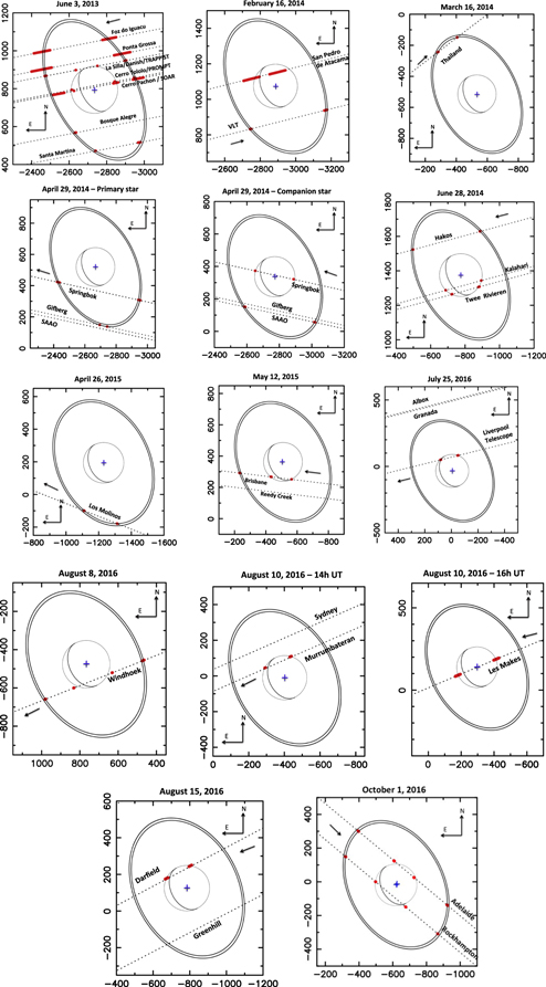
Figure 1. Reconstructed geometries of the occultations. The dotted lines are the trajectories of the occulted star relative to Chariklo in the plane of sky as seen from each station (the arrow indicates the direction of the apparent movement of the star). The red segments are the  level error bars on each chord extremity, derived from the corresponding error bars on the timings (see Tables 3–5). For those plots, we use the pole position and radii from Braga-Ribas et al. (2014):
  km,
km,  km, and
  km. The center of the ring system (blue cross) in each panel represents the offset in right ascension and declination between the predicted and observed positions of Chariklo relative to the occulted star, as given in Table 1. This offset was used to improve Chariklo’s ephemeris.
Download figure:
Standard image High-resolution imageIf the rings are not circular, this will impact their pole position and will eventually be visible as discrepancies between observations and predictions. The pole position problem is discussed further in Section 3.4.
Note that some stations did not detect any ring occultations, whereas they should have, considering the occultation geometry; see Reedy Creek on 2015 May 12 and Sydney on 2016 August 10. Data analysis shows that those non-detections are actually consistent with the low signal-to-noise-ratio (S/N) obtained at those stations. Thus, secondary events have always been detected if the S/N was high enough. This leads us to conclude that C1R (which always dominates the profile) is continuous. The same conclusion on C2R is more ambiguous as C2R was usually blended together with C1R. Nevertheless, we will assume that C2R is continuous in this paper.
2.3. Data Reduction
After a classical data processing that included dark subtraction and flat fielding, aperture photometry provided the stellar flux as a function of time (the date of each data point corresponding to the mid-exposure time), the aperture being chosen to maximize the S/N. The background flux was estimated near the target and nearby reference stars, and then subtracted, so that the zero flux corresponds to the sky level. The total flux from the unocculted star and Chariklo was normalized to unity after fitting the light curve by a third- or fourth-degree polynomial before and after the event. In all cases, a reference star (brighter than the target) was used to correct for low-frequency variations of the sky transparency.
The light curves are displayed in Figures 2 and 4, each of them providing a one-dimensional scan across Chariklo’s system, as projected in the sky plane. In some cases, the readout time between two frames caused a net loss of information as photon acquisition was interrupted during those “dead time” intervals. The flux statistics provides the standard deviation of the signal, which defines the  error bar on each data point that was used later for fitting diffraction models to the ingress and egress events. Note that during an occultation by the main body the stellar flux drops to zero, but the flux in the light curve is not zero, as it contains Chariklo’s contribution, and in one case, the flux from a nearby companion star; see below.
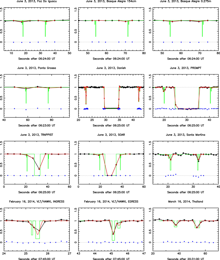
Figure 2. Best fits to the ring and main body occultations. The black dots are the data points of the light curves (the vertical axis represents the normalized flux). They are normalized between zero and unity. The latter corresponds to the full flux from Chariklo and the occulted star. The dotted lines correspond to the zero level of the occulted star. The green curves are the best-fitting square-well models used to generate the synthetic profiles, plotted in red. The physical characteristics of the rings extracted from these plots are listed in Tables 3 and 4. The blue dots are the residual between the synthetic light curves and the data at each data point. Figure 3 shows the fits of the remaining rings occultations.
Download figure:
Standard image High-resolution image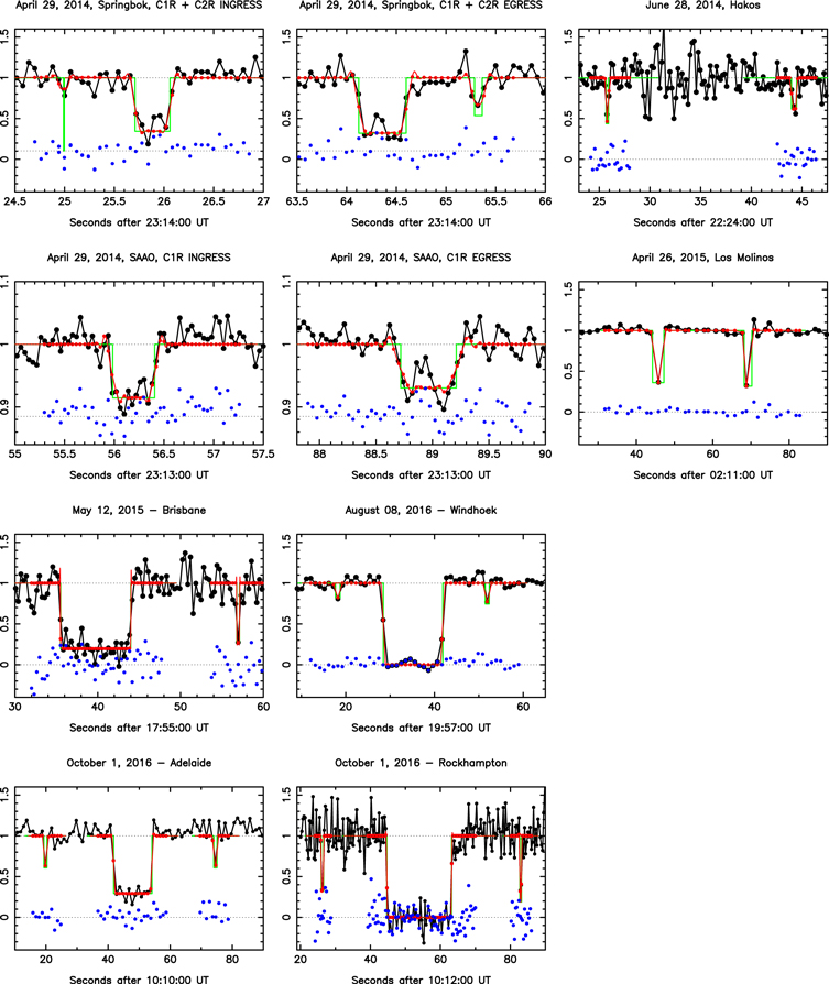
Figure 3. Best fits to the ring and main body occultations (following and completing Figure 3). Same legend as in Figure 3, except in the case of the occultation on 2014 April 29, where two stars were occulted. In this case, unity corresponds to the flux of the two stars and Chariklo. As SAAO observed an occultation of a secondary star (see Section 2.4), its vertical scale is different from other light curves, for better viewing.
Download figure:
Standard image High-resolution image2.4. The Case of the Double Star of 2014 April 29
This event, observed from South Africa (see Table 1), revealed that the occulted star was a binary. As seen from Springbok, the primary star (“A”) was occulted by C1R and C2R (but missed the main body), while the fainter companion star (“B”) disappeared behind Chariklo along an essentially diametric chord at Springbok (Figure 1). Because component B was about nine times fainter than A (see below), and considering the drop in the light curve of A caused by C1R at Springbok, we expect a small drop in the light curve of only 8% due to the disappearance of component B behind C1R. This is too small to be detected, in view of the S/N of about 7 per data point obtained at that station (Figure 3).
Meanwhile, in Gifberg, we obtained only a grazing occultation of the primary star by C2R (Figure 1). This provides the best profile of that ring ever recorded (see Section 3.3). Finally, at the South African Astronomical Observatory (SAAO), only component B was occulted by the rings, while the main star missed both the rings and the main body (Figure 1). However, due to the high S/N obtained at that station, the partial drop caused by the rings in component B light has about the same useful S/N as the drop in component A light as seen from the smaller telescope at Springbok.
For the Springbok light curve, we can estimate the flux ratio  between the two stars by considering the drop of light of component B caused by Chariklo. In doing so, we can neglect Chariklo’s contribution to the total flux. From Chariklo’s absolute magnitude, HV = 7.0 in 2014 (Duffard et al. 2014), and heliocentric and geocentric distances of 14.8 au and 14.1 au during the event, respectively, we obtain a Chariklo apparent magnitude of ∼18.6. This is 5.6 mag fainter than the star, which has V = 13.0 (NOMAD catalog56
), meaning that Chariklo contributed less than 0.6% to the total flux, a negligible value at our level of accuracy.
between the two stars by considering the drop of light of component B caused by Chariklo. In doing so, we can neglect Chariklo’s contribution to the total flux. From Chariklo’s absolute magnitude, HV = 7.0 in 2014 (Duffard et al. 2014), and heliocentric and geocentric distances of 14.8 au and 14.1 au during the event, respectively, we obtain a Chariklo apparent magnitude of ∼18.6. This is 5.6 mag fainter than the star, which has V = 13.0 (NOMAD catalog56
), meaning that Chariklo contributed less than 0.6% to the total flux, a negligible value at our level of accuracy.
The fractional drop observed during the occultation of B by Chariklo provides its partial contribution to the total stellar flux,  (Figure 4). This implies a flux ratio
  , as measured by the Texas Instruments TC247 array used at Springbok (in broadband mode, no filter). This directly provides the baseline level for the occultations of A by the rings (Figures 4 and 7), i.e., the level that corresponds to a total disappearance of component A.
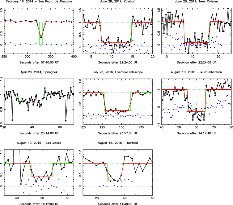
Figure 4. Same as Figure 3, but for events with only main body detections.
Download figure:
Standard image High-resolution imageA similar calibration is not possible for the SAAO ring events, as that station did not record an occultation by the main body. Moreover, the ratio  cannot be used, as the SHOC instrument (see Coppejans et al. 2013) used at SAAO (also in broadband mode) has a different spectral response, so that the ratio depends on the color of the two stars.
To proceed, we used the B, V, K magnitudes of the star (taken from the Vizier page, in the NOMAD catalog). We generated a combined synthetic spectra energy distribution of the two components, and used various (and separate) effective temperatures  for A and B. The effect of interstellar reddening has been parametrized using the color excess
  . We adopted the classical total to selective extinction parameter RV = 3.1 for Milky Way dust from Fitzpatrick (1999). The relative contributions of each component were adjusted in order to fit both the observed magnitude of the star and the flux ratio as observed with the TC247 array. Finally, accounting for the spectral response of the Andor array, we can then estimate the ratio
  for that detector.
A difficulty stems from the fact that there is a degeneracy between the effective temperatures assumed for the two components,  and
and  . The star B cannot be much cooler than A, otherwise its diameter would be larger and strong signatures in the near-IR would appear in the composite spectrum. We have opted for a difference
  K, and assume that the two stars are on the main sequence. We find a good fit to the observed magnitudes with
  K and
K and  K, and then a ratio
  , corresponding to a contribution to the total flux of
  for component A, where the error bar is estimated from the typical possible ranges for
  and
and  .
.
Finally, we can estimate the apparent diameter of each component projected at Chariklo’s distance:  km and
  km. Those values will be used latter when fitting the ring profiles with models of diffracting, semi-transparent bands.
Assuming the ring radii and pole orientation of Braga-Ribas et al. (2014; see also Section 2.2) and using the ring detections in Springbok, Gifberg, and SAAO, we deduce that star B was at angular distance 20.6 mas from star A as projected in the sky plane, with position angle  relative to the latter (where P is counted positively from celestial north toward celestial east).
3. Ring Events Analysis
3.1. Profile Fitting
In order to determine accurate and consistent timings of the ring occultations, we use a “square-well model” in which each ring is modeled as a sharp-edged, semi-transparent band of apparent opacity  (along the line of sight) and apparent width (in the sky plane) W⊥. We use the numerical schemes described in Roques et al. (1987) to account for Fresnel diffraction, stellar diameter projected at Chariklo’s distance, finite bandwidth of the CCD, and finite integration time of the instrument. Finally, considering projection effects, we can derive the physical parameters of the ring (radial width, normal opacity, etc.) and orbital elements; see the Appendix for details.
For the sake of illustration, we give various parameters of interest in the case of the 2014 April 29 occultation. The Fresnel scale  for Chariklo’s geocentric distance at this epoch,
  km is 0.83 km, for a typical wavelength of
  μm. The projected stellar diameters have been estimated above to be 0.199 ± 0.015 km and 0.092 ± 0.015 km for the primary star and secondary star, respectively (see Section 2.4). The smallest cycle time used during that campaign was 0.04 s (at SAAO), corresponding to 0.5 km traveled by the star relative to Chariklo in the celestial plane. Consequently, the light curves are dominated by Fresnel diffraction, but the effects of the stellar diameters and finite integration time remain comparable. Similar calculations for the 12 other occultations show that the effect of finite integration time dominated in all those cases.
The synthetic ring profiles are then fitted to the observations so as to minimize the classical  function:

where Φ is the flux, i refers to the  data point, “obs” refers to observed, “calc” refers to calculated, and σ the
  level error of the
  data point. The free parameters of the model are described in the next subsection. The
  error bar on each parameter is estimated by varying this particular parameter to increase
  from the best-value
  to
to  ; the other parameters are set free during this exploration.
3.2. Mid-times and Widths of the Rings
The best-fitting square-well model described above provides the relevant parameters that depend on the occulting object. Three cases are possible: occultations by the (1) main body, (2) resolved rings, and (3) unresolved rings. The relevant parameters in each case are, respectively, (1) the times of ingress and the egress of the star behind the body, (2) the mid-time of the occultation t0, the radial width reprojected in the plane of the rings, Wr, and the local normal opacity pN for each ring (see the Appendix for details), and (3) the mid-time of the occultation. Those parameters are listed in Table 3 (resolved ring events), Table 4 (unresolved ring events), and Table 5 (main body events). The best fits for each occultation are plotted in Figures 2 and 3 (ring occultations) and Figure 4 (main body occultations).
Table 3. Ring Occultation Timings and Derived Physical Parameters (Resolved Events)
| Date | Event | t0 UTa |
 b
b
|
 b
b
|
Lc |
 d
d
|
 e
e
|
 e
e
|
|---|---|---|---|---|---|---|---|---|
| (km s−1) | (km s−1) | (deg.) | (km) | (km) | ||||
| C1R | ||||||||
| Jun 3, 2013 | Danish ingressf | 06:25:21.166 ± 0.0007 | 20.345 | 36.113 | 341.76 | 6.16 ± 0.11 | 1.90 ± 0.022 | 0.308 ± 0.003 |
| Danish egressf | 06:25:40.462 ± 0.0012 | 22.031 | 36.504 | 124.38 | 7.14 ± 0.04 | 1.73 ± 0.023 | 0.24 ± 0.004 | |
| 2014 Feb 16 | VLT ingress | 07:45:25.541
|
19.532 | 28.794 | 183.37 |

|

|

|
| VLT egress | 07:45:45.133
|
21.293 | 29.602 | 300.99 |

|

|

|
|
| 2014 Apr 29 | Springbok ingress | 23:14:25.884 ± 0.007 | 13.432 | 16.493 | 287.42 | 5.575 ± 0.398 |

|

|
| Springbok egress | 23:15:04.362 ± 0.006 | 10.720 | 16.655 | 157.83 |

|

|

|
|
| SAAO ingress | 23:13:56.191 ± 0.007 | 12.756 | 13.895 | 266.656 | 5.68 ± 0.2 |

|

|
|
| SAAO egress | 23:14:28.964 ± 0.008 | 9.260 | 14.249 | 198.899 | 6.625 ± 0.2 |

|

|
|
| C2R | ||||||||
| Jun 3, 2013 | Danish ingressf | 06:25:20.765 ± 0.011 | 20.412 | 36.283 | 341.76 |

|
0.168 ± 0.02 |

|
| Danish egressf | 06:25:40.847 ± 0.006 | 22.029 | 36.632 | 124.38 |

|
0.228 ± 0.02 |

|
|
| 2014 Feb 16 | VLT ingress | 07:45:25.285
|
19.532 | 28.794 | 183.37 |

|

|

|
| VLT egress | 07:45:45.473
|
21.293 | 29.602 | 300.99 |

|

|

|
|
| 2014 Apr 29 | Springbok ingress | 23:14:24.990 ± 0.020 | 13.430 | 16.460 | 287.42 |

|

|

|
| Springbok egress | 23:15:5.324 ± 0.019 | 10.722 | 16.620 | 157.832 |

|

|

|
|
| Gifberg ingressg | 23:14:30.109
|

|

|
227.190 |

|

|

|
|
| Gifberg egressg | 23:14:33.750 ± 0.008 |

|

|
217.761 |

|

|

|
|
Notes.
at0 is the mid-time of the event in hours:min:sec. The error bars quoted are given at the level.
b
level.
b
 and vr are, respectively, the perpendicular velocity in the sky plane and the radial velocity in the ring plane.
cL is the true longitude counted from the J2000 ring plane ascending node.
dWr is the radial width, measured in the plane of the rings.
eEp is the equivalent width:
and vr are, respectively, the perpendicular velocity in the sky plane and the radial velocity in the ring plane.
cL is the true longitude counted from the J2000 ring plane ascending node.
dWr is the radial width, measured in the plane of the rings.
eEp is the equivalent width:  , where pN is the normal opacity in the plane of the rings.
fTimings given by Braga-Ribas et al. (2014).
gAs the occultation was grazing, the velocity changes consequently between ingress and egress, and to give fixed values is not relevant in this case (see Section 3.2).
, where pN is the normal opacity in the plane of the rings.
fTimings given by Braga-Ribas et al. (2014).
gAs the occultation was grazing, the velocity changes consequently between ingress and egress, and to give fixed values is not relevant in this case (see Section 3.2).
Download table as: ASCIITypeset image
Table 4. Ring Occultation Timings and Derived Physical Parameters (Unresolved Events)
| Date | Event | t0 UTa |
 (km s−1)a (km s−1)a
|
vr (km s−1)a | L(deg)a | Ep (km)a |
|---|---|---|---|---|---|---|
| 2013 Jun 3 | Iguacu ingress | 06:24:17.5 ± 1.7b | 18.059 | 28.899 | 2.44 |

|
| Iguacu egress | 06:24:34.1 ± 2.0b | 21.246 | 30.446 | 104.20 |

|
|
| Bosque Alegre 154 egress | 06:25:11.44 ± 0.14b | 18.889 | 32.663 | 176.11 |

|
|
| Ponta Grossa ingress | 06:23:58.6 ± 2.5b | 19.781 | 34.398 | 348.04 |

|
|
| Ponta Grossa egress | 06:24:18.0 ± 2.5b | 21.965 | 35.520 | 120.30 |

|
|
| PROMPT ingress | 06:25:20.0.46 ± 0.011b | 21.373 | 38.269 | 326.56 |

|
|
| Santa Martina ingress | 06:25:21.03 ± 0.29b | 17.556 | 18.537 | 264.53 |

|
|
| Santa Martina egress | 06:25:31.811 ± 0.025b | 14.605 | 22.124 | 200.07 |

|
|
| SOAR ingress | 06:25:18.8 ± 1.3b | 21.444 | 38.320 | 325.16 |

|
|
| SOAR egress | 06:25:38.4 ± 1.4b | 21.660 | 38.310 | 140.37 |

|
|
| Bosque Alegre C11 ingress | 06:24.55.45 ± 1.85b | 21.522 | 30.340 | 287.37 |

|
|
| Bosque Alegre C11 egress | 06:25:09.45 ± 1.75b | 17.882 | 30.062 | 183.50 |

|
|
| TRAPPIST ingress | 06:25:20.9 ± 1.9b | 20.293 | 36.229 | 341.31 |

|
|
| 2014 Mar 16 | Thailand ingress | 20:31:37.640 ± 1.33 | 3.656 | 3.821 | 95.06 |

|
| Thailand egress | 20:31:53.885 ± 0.175 | 3.990 | 4.290 | 60.85 |

|
|
| 2014 Jun 28 | Hakos ingress | 22:24:25.796 ± 0.041 | 19.127 | 28.619 | 5.064 |

|
| Hakos egress | 22:24:44.218 ± 0.035 | 20.971 | 29.744 | 117.061 |

|
|
| 2015 Apr 26 | Los Molinos ingress | 02:11:45.707 ± 0.058 | 3.503 | 3.513 | 238.857 |

|
| Los Molinos egress | 02:12:09.195 ± 0.070 | 2.957 | 3.989 | 199.749 |

|
|
| 2015 May 12 | Brisbane egress | 17:55:56.823 ± 0.012 | 11.823 | 16.567 | 357.23 |

|
| Aug 8, 2016 | Windhoek (CHMO) ingress | 19:57:18.209 ± 0.249 | 15.920 | 21.878 | 332.963c |

|
| Windhoek (CHMO) egress | 19:57:51.870 ± 0.382 | 15.216 | 21.950 | 180.196c |

|
|
| 2016 Oct 1 | Rockhampton ingress | 10:12:26.284 ± 0.072 | 10.795 | 13.121 | 123.960 |

|
| Rockhampton egress | 10:13:22.928 ± 0.049 | 12.573 | 13.146 | 278.911 |

|
|
| Adelaide ingress | 10:10:19.826 ± 0.186 | 12.421 | 12.597 | 91.347 |

|
|
| Adelaide egress | 10:11:14.558 ± 0.218 | 9.942 | 12.651 | 311.914 |

|
|
Notes.
aSame parameters as in Table 3. bTimings given by Braga-Ribas et al. (2014). cTwo geometries are possible for this occultation. We arbitrarily choose the one closest to the prediction. The other geometry provides different longitudes: and
and  .
.
Download table as: ASCIITypeset image
Table 5. Occultation Timings for the Main Body
| Date | Event | tingress UT | tegress UT |
|---|---|---|---|
| 2013 Jun 3 | Danish | 06:25:27.861 ± 0.014 | 06:25:33.188 ± 0.014 |
| PROMPT | 06:25:24.835 ± 0.009 | 06:25:35.402 ± 0.015 | |
| TRAPPIST | 06:25:27.893 ± 0.019 | 06:25:33.155 ± 0.007 | |
| SOAR | 06:25:24.34 ± 0.59 | 06:25:34.597 ± 0.009 | |
| 2014 Feb 16 | San Pedro de Atacama | 07:45:27.450 ± 0.6 | 07:45:31.125 ± 0.57 |
| 2014 Jun 28 | Kalahari | 22:24:07.383 ± 0.126 | 22:24:14.854 ± 0.096 |
| Twee Rivieren | 22:24:06.689 ± 0.093 | 22:24:16.481 ± 0.105 | |
| 2014 Apr 29 | Springbok | 23:14:30.02 ± 0.075 | 23:14:48.03 ± 0.075 |
| 2015 May 12 | Brisbane | 17:55:35.530 ± 0.010 | 17:55:44.135 ± 0.075 |
| 2016 Jul 25 | Liverpool Telescope | 23:59:05.494 ± 0.054 | 23:59:12.310 ± 0.054 |
| 2016 Aug 8 | Windhoek (CHMO) | 19:57:28.469 ± 0.042 | 19:57:41.886 ± 0.045 |
| 2016 Aug 10-14 hr UT | Murrumbateran | 14:18:35.030 ± 0.3 | 14:18:45.145 ± 0.125 |
| 2016 Aug 10-16 hr UT | Les Makes | 16:42:51.305 ± 0.530 | 16:43:07.917 ± 0.848 |
| 2016 Aug 15 | Darfield | 11:38:27.465 ± 0.385 | 11:38:38.019 ± 0.873 |
| 2016 Oct 1 | Rockhampton | 10:12:44.664 ± 0.041 | 10:13:03.199 ± 0.051 |
| Adelaide | 10:10:41.818 ± 0.118 | 10:10:54.102 ± 0.064 |
Note. The error bars quoted are given at the  level.
Download table as: ASCIITypeset image
The grazing occultation by C2R recorded in Gifberg (Figure 1) requires a special analysis. In this geometry, the radial velocity of the star relative to the ring changes significantly during the event (while it is assumed to be constant for all other events). To account for this peculiarity, we first converted the light curve (time, flux) into a profile ( , flux), where
  is the radial distance to the point of closest approach to Chariklo’s center (in the sky plane). Then we can apply the square-well model as explained in Section 3.1, except that the flux is now given in terms of
  , instead of time. The best fits for the ingress and egress are plotted in Figure 5.
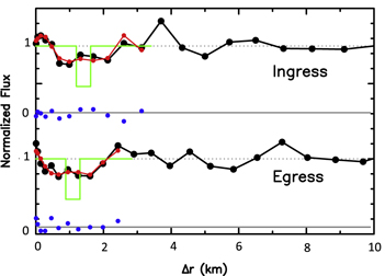
Figure 5. Fits to the grazing event in Gifberg (2014 April 29) using a common width ( km and
  ) for both rings into the
  level (see Table 3). The star motion relative to C2R was grazing, so that its velocity perpendicular to the ring changed significantly during the occultation. In this case, it is therefore necessary to express the flux against the distance to the point of closest approach to Chariklo’s center in kilometers in the sky plane,
  . Other than that, the color conventions and vertical axis are the same as in Figure 2.
Download figure:
Standard image High-resolution imageTable 3 summarizes the values of Wr for each resolved profile. Figure 6 shows Wr versus the true longitude L counting from the ascending node. Accounting for the most constraining events, Wr varies between 5 and 7.5 km in C1R and between 0.05 and 1 km in C2R (at the  level). Figure 6 could constrain the proper mode of the rings. Unfortunately, the true longitude L plotted in Figure 6 (and later in Figure 10) is not the correct quantity to use in order to detect the m = 1 proper modes (the true anomaly
  should be used instead of L, where ϖ is the longitude of periapse). As the precession rates of the rings are unknown, no conclusion can be made. Nevertheless, those width variations are observed both for a given occultation at different longitudes and for different occultations at different dates; see Figure 7. The implications are discussed in Section 6.
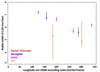
Figure 6. Variation of the C1R radial width (and  error bars) with true longitude L counted from the J2000 ring plane ascending node for resolved events.
Download figure:
Standard image High-resolution image3.3. Ring Inner Structures
Figure 8 shows the best radial profiles of the rings that we have obtained so far, taken from the discovery observation of 2013 June 3 and the 2014 April 29 event. They are currently the only profiles that clearly resolve C1R from C2R, and in the case of the 2014 April 29 event, the only profiles that resolve C1R. A W-shape structure inside C1R is clearly seen at egress in the Springbok and SAAO profiles, and marginally detected in the Springbok ingress profile, while being absent (to within the noise) in the SAAO ingress profile.
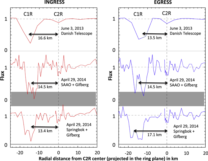
Figure 7. Best radial profiles of the rings C1R and C2R. The profiles have been plotted arbitrarily against the radial distance (in the ring plane) to the center of the C2R profile, using the pole position of Braga-Ribas et al. (2014). This choice enhances possible changes in the relative distances of the two rings, due, for instance, to eccentricities of C1R and/or C2R. The horizontal dashed lines correspond to the unocculted star + Chariklo flux. The horizontal gray boxes correspond to the respective zero stellar fluxes. The thickness of the gray box indicates the uncertainty of the photometric calibrations; see the text for details (Section 2.4). The left (right) panel corresponds to ingress (egress). Top panels: the 2013 June 3 profiles from the Danish Telescope. Middle and bottom panels: montages constructed from the 2014 April 29 event. The Gifberg profiles showing C2R have been combined with the SAAO light curve (middle panel) and Springbok light curve (bottom panel).
Download figure:
Standard image High-resolution imageNote that small (2–4 km) variations of radial distances between the two rings are visible in Figure 8. The average gap distance between the two rings on the six profiles is thus 14.8 km.
Since the origin of radial distance has been fixed arbitrarily on the center of C2R, it is not possible to attribute those variations to an eccentricity of C1R, C2R, or both. Note also that the April 29 profiles are montages obtained by juxtaposing the profiles of C1R recorded at Springbok and SAAO, and the profile of C2R recorded in Gifberg. So, they scan different ring longitudes, and conclusions based on this plot can only be qualitative.
3.4. Ring Pole
By analogy with their Uranian counterparts, we expect that Chariklo’s ring orbits essentially have elliptical shapes, corresponding to a normal mode with an m = 1 azimuthal harmonic number. Moreover, other modes with higher values of m are possible and the two rings may not be coplanar. However, data on Chariklo’s rings are currently too scarce to reach those levels of detail. Instead, we have to simplify our approach, considering the observational constraints on hand.
The simplest hypothesis is to assume that the two are circular, concentric, and coplanar. Then, their projections on the sky plane are ellipses characterized by M = 5 adjustable parameters: the apparent semimajor axis  , the coordinates of the ellipse’s center
  , the apparent oblateness
  (where
  is the apparent semiminor axis), and the position angle P of the semiminor axis
  . For circular rings,
  , where B is the ring opening angle (B = 0 and
  corresponding to edge-on and pole-on geometries, respectively).
Note that  is related to the offsets in right ascension and declination between the predicted and observed positions of the object, relative to the occulted star. The positions of Chariklo deduced from
  —at prescribed times and for given star positions—are listed in Table 1. They can be used to improve Chariklo’s ephemeris, once the star positions are improved, using the DR1 Gaia catalog and its future updates.
This circular ring model requires at least  data points in order to provide a unique solution for the ring radius a (coincident with
  ) and its J2000 pole position
  . Only the 2013 June 3 discovery observation with seven chords (and thus N = 14 data points corresponding to the chord extremities) has sufficient constraints to provide unambiguous ring orbits. More precisely, as only one instrument (Danish telescope) could resolve the rings C1R and C2R in 2013, this multichord event mainly determines the orbit of C1R, which largely dominates the usually blended ring profiles. Then we assumed that C2R is coplanar with C1R and separated radially from it by a constant distance
  km (Braga-Ribas et al. 2014).
The 2014 April 29 event provides two chords (N = 4 data points) on C2R. This allows us to definitely eliminate one of the pole positions derived from the 2013 event. Actually, determining the angles B and P at a given date provides two possible pole positions, 1 and 2, depending on which part of the rings, as seen in the sky plane, is the “near arm” or the “far arm”; see Braga-Ribas et al. (2014) for details. The C2R chord observed at Springbok turned out to be longer than the longest possible length allowed by solution 2, thus confirming that the preferred solution 1 of Braga-Ribas et al. (2014), based on the long-term photometric behavior of Chariklo (see also below), was actually the correct one.
In order to constrain the pole position, even with  , we vary the couple (
 ) in a predetermined grid, while the other three parameters are adjusted in order to minimize the radial residuals in the sky plane relative to the ring center. Since the pole position is given by two parameters
  , the 68.7% confidence domain (called the
  level here) is obtained by allowing variations of the
  function from
  to
to  (Press et al. 1992), and by selecting values of a to ±3.3 km, the nominal error on the C1R and C2R radii:
  km and
  km (Braga-Ribas et al. 2014). The pole position derived from the 2014 April 29 occultation is displayed in Figure 9. Note that it is consistent with but less accurate than the pole determined in 2013.
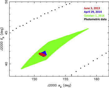
Figure 8. Constraints on ring pole. The uncertainty domains (1σ level) on the pole position ( ) for the events on 2013 June 3, 2014 April 29, and 2016 October 1 are plotted in red, blue, and green, respectively. The black dots outline the uncertainty domain derived from the long-term variations in Chariklo’s photometry (Duffard et al. 2014).
Download figure:
Standard image High-resolution imageFinally, the 2016 October 1 event also provided two chords (N = 4 data points) across the rings, but without resolving C1R from C2R (Figure 4). Thus, we assumed that the profiles are dominated by C1R, and derived the pole position displayed in Figure 9. It is again consistent with the poles of 2013 and 2014, but with larger error bars due to the ill-configured chord geometry (nearly diametric) that permits more freedom on the pole position (Figure 1).
Further constraints are in principle provided by the long-term photometric behavior of Chariklo’s system between 1997 and 2014, as compiled by Duffard et al. (2014); see their Figure 1. The observed photometric variations can be explained by the changing viewing geometry of the rings, linked itself to the pole orientation. Contrary to the occultation data, the photometric variations do not depend on the particular shape of the rings (e.g., circular versus elliptic). Fitting for the pole position and accounting for the error bars taken from Duffard et al. (2014), we obtain the possible domain shown in Figure 9. Note that it is consistent with but less accurate than all of our occultation results.
From Figure 9, we can conclude that our current data set (spanning the three-year interval 2013–2016) is consistent with circular rings that maintain a fixed pole in space, and to within the current formal error bar on the semimajor axis a (±3.3 km). Note that the extensions of the error domains for the pole position (colored regions in Figure 9) are dominated by the errors in the data (i.e., the timings of the ring occultations), not by the formal error for a quoted above. In other words, even if the ring shape were known perfectly, the pole position would not be significantly improved compared to the results shown in Figure 9. A Bayesian approach could be used to estimate the probability that the rings are elliptic, considering the data on hand and assuming a random orientation for the ring apsidal lines. Considering the paucity of data and the large number of degrees of freedom, this task remains out of the scope of the present paper. In any case, new observations will greatly help in this approach by adding more constraints on the ring shapes and orientations.
For all other single-chord detections (N = 2 data points) of the ring, neither the rings’ radii nor their pole positions can be constrained. Instead, assuming the pole orientation of Braga-Ribas et al. (2014), we determined the ring center, also assumed to coincide with Chariklo’s center of mass. Having only one ring chord introduces an ambiguity as two solutions (north or east of the body center) are possible. However, in all cases but one (2016 August 8), it was possible to resolve this ambiguity as the absence of detections made by other stations eliminated one of the two solutions. For the 2016 August 8 event, the ambiguity remains, and we give the two possible positions for Chariklo; see Table 1.
None of the single chords are longer than the longest chord expected from Braga-Ribas' et al. (2014) solution, and thus remain fully consistent with that solution.
3.5. Sharpness of C1R Edges
A striking feature of the resolved C1R profiles from the 2014 April 29 event is the sharpness of both its inner and outer edges. This is reminiscent of the Uranian rings (Elliot et al. 1984; French et al. 1991), and might stem from confining mechanisms caused by nearby, kilometer-sized shepherding moonlets (Braga-Ribas et al. 2014). In order to assess the sharpness of C1R’s edges, we use a simple model, where each edge has a stepwise profile, as illustrated in Figure 9. Instead of having an abrupt profile that goes from apparent opacity 0 to  , we add an intermediate step of radial width in the ring plane
  and opacity
  around the nominal ingress or egress times, as deduced from the square-well model described before; see also Table 3. With that definition,
  is a measure of the typical edge width, i.e., the radial distance it takes to go from no ring material to significant optical depth.
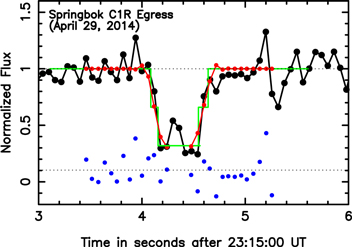
Figure 9. Measurement of the sharpness of C1R’s edges with an example taken from the Springbok egress profile (2014 April 29). The green line is the stepwise model of width  described in Section 3.5. The red dots are the resulting synthetic points (the blue dots showing the residuals). The sharpness parameters
  shown here are the maximum values that are compatible with the data at the 1σ level, with values
  km for the left (inner) edge and
  km for the right (outer) edge. Table 6 lists the values of
  obtained with the other resolved C1R profiles.
Download figure:
Standard image High-resolution imageWe explored values of  by varying the
  function (Equation (1)) from its minimum value
  to
to  . The results are listed in Table 6 and illustrated in Figure 9. Note that all edges are consistent with infinitely sharp edges (
 ) to within the
  level and that upper limits for
  are typically 1 km. No significant differences are noticeable between the inner and the outer edges, contrary to, e.g., some Uranian rings (French et al. 1991).
Table 6.
Sharpness of C1R’s Edges,  , from the 2014 Apr 29 Events
| Event | Inner Edge (km) | Outer Edge (km) |
|---|---|---|
( Level) Level) |
||
| Springbok Ingress | 1.1 | 1.1 |
| Springbok Egress | 1.2 | 1.5 |
| SAAO Ingress | 0.6 | 0.9 |
| SAAO Egress | 0.8 | 0.4 |
Download table as: ASCIITypeset image
Note finally that the width of C2R, as derived from the grazing event in Gifberg (Figure 5), is slightly smaller (∼0.7 km) than the Fresnel scale (∼0.8 km). As such, it is not possible to assess the sharpness of its edges.
4. Integral Properties of Rings: Equivalent Width and Depth
We now turn to the measure of the ring’s equivalent width Ep and equivalent depth Aτ, two quantities defined and discussed by Elliot et al. (1984) and French et al. (1991), as detailed in the Appendix. Those quantities are physically relevant, as they are related to the amount of material present in a radial cut of the ring, in the extreme cases of monolayer and polylayer rings, respectively.
The values of Ep are given in Table 3 (resolved events) and Table 4 (unresolved events). For the resolved profiles, we have plotted Ep against the radial width Wr in Figure 10. The implications in terms of mono- versus polylayer models will be discussed in Section 6. For the profiles that resolve C1R from C2R (and where both rings were detected), and those where the two profiles are blended (the majority of our observations), we have plotted the integrated  against the true longitude L (counted from the J2000 ring plane ascending node) in Figure 10. From that figure, we see that the values of
  lie in the interval 1–3 km, with no significant differences between the various measurements. In other words, no significant variations of
  with time and/or longitude are detected in our data set.
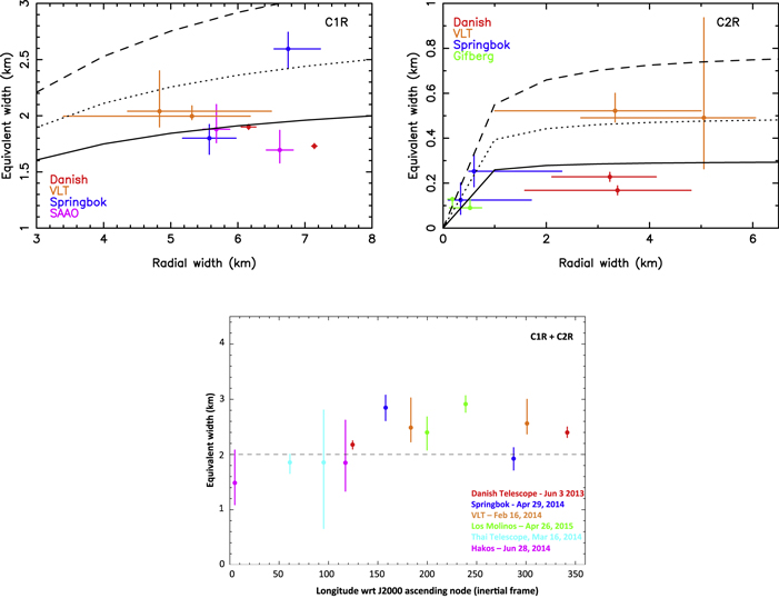
Figure 10. Top left: equivalent width Ep (using Equation (6)) of C1R vs. the radial width for resolved events. The theoretical lines Ep vs. Wr expected from a polylayer ring (see Equation 3) have been plotted in black with  km (solid line),
  km (dotted line), and
  km (dashed line). Top right: same, but for C2R. The black lines are now with
  km (solid line),
  km (dotted line),
  km (dashed line). Bottom: the integrated equivalent width
  of C1R and C2R vs. the true longitude L, counted from the J2000 ring plane ascending node, from our best events (resolved or not). As SAAO detected only a C1R occultation and Gifberg only a C2R event, they have been removed from the plot. The dashed line indicates the mean value of the data points.
Download figure:
Standard image High-resolution imageIn this preliminary study, the rings are considered as one entity C1R + C2R but further studies should treat them independently to derive conclusions on the structure of each of them.
5. Search for Faint Ring Material
The best light curve available in terms of photometric quality is from the Danish Telescope. It was acquired at a rate of 10 frames per second during the 30 minutes bracketing the occultation of 2013 June 3 (Braga-Ribas et al. 2014). It can be used to search for additional material orbiting Chariklo, assuming semi-transparent, uninterrupted, and permanent rings coplanar to C1R and C2R.
For this purpose, we consider the equivalent width Ep(i) of the putative ring material intercepted during the acquisition interval  corresponding to the
  data point, and counted radially in the ring plane. Using the results of the Appendix (see also Boissel et al. 2014 for details), we obtain

where  is the radial interval travelled by the star during
  (projected in the ring plane), and where
  is the normalized stellar flux. Due to projection effects, the value of
  varied between the extreme values of 3–4 km during the acquisition interval, which sets the radial resolution of this particular data set.
The values of Ep(i) versus the radial distance r is displayed in Figure 11. Note that the light curve probes radial distances of up to ∼12,000 km, about 30 times the ring radii. Using bins of width 60 km, we evaluate the variance of the difference between two consecutive points in each box, thus eliminating low-frequency variations of Ep(i). Dividing this variance by two (to account for the fact that the data points are uncorrelated) and taking the square root, we obtain the  level, the standard deviation of Ep(i), denoted
  ; see the red line in Figure 11. The value of
  remains stable in the entire range considered here, with typical values of 20 m. Thus, at the
  level, we do not detect narrow (
 km) rings coplanar with C1R and C2R with equivalent width larger than about 20 m. This is about 10 times fainter than the equivalent width of C2R (Figure 10). Note that this limit corresponds to extreme cases of either opaque rings with width ∼ 20 m, or semi-transparent rings of width ∼3–4 km and normal opacity 0.007–0.005, and all the intermediate solutions that keep Ep(i) at 20 m.
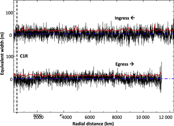
Figure 11. Search for faint ring material using the Danish light curve (2013 June 3 event). Black solid lines: the equivalent width Ep of possible ring material (Equation (2)) vs. the radial distance (in the ring plane) to Chariklo’s center. The data points corresponding to the detections of the main body and C1R and C2R have been removed for clarity (for comparison,  km and
  m—see Table 3). The black vertical dotted line indicates the location of C1R, and the horizontal dashed−dotted blue lines mark the zero level for Ep. Red solid lines: standard deviation (
 level) of Ep(i) estimated in bins of width 60 km; see the text for details.
Download figure:
Standard image High-resolution image6. Concluding Remarks
We detected Chariklo and/or its rings during a total of 13 stellar occultations between 2013 and 2016. They demonstrate beyond any doubt that this Centaur is surrounded by a system of two flat rings, C1R and C2R. All of the observations on hand are consistent with the circular ring solution of Braga-Ribas et al. (2014), with C1R orbiting 391 ± 3 km from Chariklo’s center and with C2R orbiting outside C1R at an average distance of 14.8 km (Figure 7). This definitely rules out interpretations of the initial observation of 2013 June 3 as a 3D dust shell or a set of cometary-type jets being ejected from the surface of the body. In fact, the changing aspect of the rings seen during the occultations is entirely attributable to the changing position of Chariklo relative to Earth, with a ring pole position that remains fixed in space (Figure 8).
Our best resolved observation (2014 April 29) reveals a W-shaped structure inside the main ring C1R (Figure 7). Moreover, the radial width Wr of C1R measured from the best profiles exhibits significant variations with longitude, with a peak to peak variation of  km between 5 and 7.5 km; see Table 3 and Figure 6. All of the resolved profiles of C1R exhibit edges that are consistent with infinitely sharp boundaries, once diffraction and star diameter effects are accounted for. The typical 1σ upper limit for the edge transition zones is about one kilometer (Table 6 and Figure 9). Note finally that none of our observations permits the profile of ring C2R, whose width is constrained between 100 m and 1 km (Figure 10), to be resolved.
Remarkably, the properties of C1R (W-shaped profile, variation of width with longitude, and sharp edges) are reminiscent of the narrow eccentric ringlets found around Saturn (French et al. 2016) or Uranus (Elliot et al. 1984; French et al. 1991). The maintenance of apse alignment could be due to self-gravity (Goldreich & Tremaine 1979), viscous effects at the edges (Chiang & Goldreich 2000), or a combination of self-gravity and viscous effects (Mosqueira & Estrada 2002). If validated, those models may provide insights into the physical parameters of the ring. For instance, the overdensities of material at some hundreds of meters from the edges (as seen in Figure 7) is predicted by viscous models and deserve more detailed observational support in the case of Chariklo. Also, the measure of the eccentricity gradient across the rings, qe, could be related to the surface density of the ring material, once Chariklo’s dynamical oblateness J2 is known (Pan & Wu 2016). However, our current data set is too fragmentary to draw any reliable conclusions in that respect, since both a comprehensive ring orbit model and knowledge of Chariklo’s J2 are missing.
In their simplest forms, the Saturn or Uranus ringlets are described as sets of nested elliptical streamlines, with a width that varies as ![${W}_{r}=[1-{q}_{e}\cos (f)]\delta a$](https://content.cld.iop.org/journals/1538-3881/154/4/144/revision1/ajaa830dieqn279.gif) , where f is the true anomaly,
, where f is the true anomaly,  measures the eccentricity gradient across the ring, and
  and
and  being the changes of the semimajor axis a and eccentricity e across that ring. Consequently, the interpretation of Figure 6 remains ambiguous, since only the true longitude corresponding to the events is currently known, while the true anomaly f is unknown. In fact, any (expected) apse precession between observations impairs a correct interpretation of that figure. At this point, only the total eccentricity variation across the ring can be estimated, i.e.,
  from the estimations of Wr and a given above. This sets a lower limit of the same order for e, close to the eccentricity of Uranus’
 ring, 0.008 (French et al. 1991).
A much better case for modeling the rings would be to derive Wr versus the ring radial excursion r–a relative to the mean radius r. The formula above predicts a linear behavior. Unfortunately, the ring center is currently undetermined: we assume, on the contrary, a circular ring to derive it and determine its pole. The fact that the circular hypothesis provides satisfactory fits to our data, to within the accuracy of C1R’s radius determination (some ±3 km), suggests that r–a should also vary by a few kilometers at most. In any case, the degeneracy between the ring eccentricity and its pole position can be lifted by obtaining several multichord occultations and more accurate pole positions than shown in Figure 8 (and thus distinguish between projection and eccentricity effects). Also, as apsidal precession rates are expected to be of the order of a couple of months (Sicardy et al. 2016); observations closer than that in time should be done to derive Chariklo’s J2.
Turning now to the integral properties of the rings, we have determined the equivalent widths Ep of C1R and C2R, when resolved, and the sum of the two when unresolved (Figure 10). We see that C1R, with  km, contains about 10 times more material than C2R,
  km. On the one hand, if the equivalent width is constant within the radial width, the ring can be considered a monolayer (French et al. 1986), as no shadowing by neighboring particules occurs (except in the nearly edge-on view). On the other hand, if the ring is polylayer, the equivalent depth is independent of Wr. In that latter case, the equivalent width can be expressed as a function of ring width Wr and the constant value of equivalent depth
  :
:

(this equation, based on the work of French et al. 1986, has been corrected by a factor of 2 in optical depth due to the diffraction by ring particules—see the Appendix). Figure 10 shows Ep versus Wr assuming several values of  between 1.15 and 2 km for C1R and between 0.15 and 0.4 km for C2R (no real measurement of this parameter has been made in this work; the lines show the expected trends—see the Appendix). Contrary to French et al. (1986), the data do not allow one to dinstinguish between Ep and Aτ constant within the radial width. Thus, no choice between the mono- or polylayer models can be made.
Finally, we searched for a faint ring of material around the already discovered rings. The best data set on hand provides 1σ upper limits of ∼20 m for the equivalent width of narrow (<3–4 km physical width) rings coplanar with C1R and C2R, up to distances of 12,000 km (counted in the ring plane). Note that in 2015, direct images of Chariklo have been recorded using HST and SPHERE (Sicardy et al. 2015a, 2015b). The goal was to image the rings and/or look for possible shepherd satellite(s) and jets. Considering material of the same albedo as the rings (p = 0.1), the following limits have been inferred: (1) no satellite bigger than ∼2 km (being brighter than  ) up to 6400 km (∼8 times the ring size) from Chariklo’s center, (2) no satellite bigger than ∼1 km (
 ) up to 8 arcsec; for comparison the Hill radius is 7.5 arcsec, and (3) no jet, coma, or material brighter than
  corresponding to jets of width ∼10 km or material of optical depth of around
  per pixel. Note that HST resolution did not allow looks closer than 1000 km from Chariklo’s center, so the rings were not detected.
Future observations will benefit greatly from the Gaia catalog. A flavor of it has been provided by the Gaia-based prediction of the 2016 October 1 occultation, which turned out to be correct to within 5 mas in declination (respectively, 9 mas in right ascension), corresponding to about 50 km (respectively, 90 km). The improvement of Chariklo’s orbit stemming from successful occultation observations and the sub-milliarcsecond accuracy of forthcoming Gaia catalogs will provide predictions accurate to the few-kilometer level. This will allow a much better distribution of stations (using portable instruments), with an optimal ring longitude coverage aimed at improving the ring orbital models. It will also be possible to plan multiwavelength observations to constrain the ring particle sizes. Multiwavelength instruments are rare and difficult to obtain unless a strong case is made, based on reliable predictions. Higher S/N light curves will also be obtained in order to calculate the equivalent depths of both rings and definitely answer whether the rings are monolayer or polylayer. Finally, the Gaia catalog will allow a much better coverage of Chariklo’s limb, which is currently poorly mapped. The general shape and local irregularities of the body will in turn have important consequences for a better understanding of the ring dynamics.
The authors acknowledge support from the French grants “Beyond Neptune” ANR-08-BLAN-0177 and “Beyond Neptune II” ANR-11-IS56-0002. Part of the research leading to these results has received funding from the European Research Council under the European Community’s H2020 (2014–2020/ERC Grant Agreement No. 669416 “LUCKY STAR”). This work is partly based on observations performed at the European Southern Observatory (ESO), proposals 092.C-0186(B) and 092.C-0186(C), and on observations made at the South African Astronomical Observatory (SAAO). This work has made use of data obtained at the Thai National Observatory on Doi Inthanon, operated by NARIT. Technical support was provided by G. Hau and P. Kabath for the 2014 February 16, observation at ESO/VLT, and by G. Román for the 2016 July 25 observation with the Dobson 60 cm telescope at Granada. A.M. acknowledges the use of Caisey Harlingten’s 50 cm telescope for the 2014 February 16 occultation. The 50 cm telescopes used for the Hakos observations belong to the IAS observatory at Hakos/Namibia. E.J. is an FNRS Research Associate. TRAPPIST is a project funded by the Belgian Fund for Scientific Research (Fonds National de la Recherche Scientifique, FRS-FNRS) under grant FRFC 2.5.594.09. F.A.P. and P.-D.J. thank the Dunedin Astronomical Society. E.M. acknowledges support from the Contrato de subvención 205–2014 Fondecyt—Concytec, Perú. M.A. thanks CNPq (Grants 473002/2013-2 and 308721/2011-0) and FAPERJ (Grant E-26/111.488/2013). G.B.-R. acknowledges the support of the CAPES (203.173/2016) and FAPERJ/PAPDRJ (E26/200.464/2015-227833) grants. R.V.-M. thanks grants CNPq-306885/2013, Capes/Cofecub-2506/2015, and FAPERJ: PAPDRJ-45/2013 and E-26/203.026/2015. The research leading to these results has received funding from the European Union’s Horizon 2020 Research and Innovation Programme, under grant agreement No. 687378, project SBNAF. The authors acknowledge the use of Sonja Itting-Enke’s C14 telescope and the facilities at the Cuno Hoffmeister Memorial Observatory (CHMO), the use of the Skywatcher 16″ telescope of the Deutsche Höhere Privatschule (DHPS) in Windhoek, and the use of the Meade 14 telescope of Space Observation Learning (Rob Johnstone). Funding from Spanish grant AYA-2014-56637-C2-1-P is acknowledged, as is the Proyecto de Excelencia de la Junta de Andalucía, JA 2012-FQM1776. J.I.B.C. acknowledges CNPq grants 308489/2013-6 and 308150/2016-3. The research leading to these results has received funding from the European Union's Horizon 2020 Research and Innovation Programme, under Grant Agreement N. 687378, project SBNAF.
Appendix: Equivalent Width and Equivalent Depth Definitions
We define  as the apparent opacity of the ring. It measures the fractional drop of stellar flux
  as observed from Earth (where I0 and I are the incident and transmitted fluxes, respectively). Thus,
  means a transparent ring and
  means an opaque ring. By “apparent,” we mean here as observed from Earth in the plane of the sky. The apparent quantities will be primed hereafter to distinguish them from the actual quantities at the level of the ring; see below. The apparent ring optical depth is defined as
  .
.
Appropriate transformations, accounting for the ring opening angle B and distance D to the ring, must be applied to derive the opacity pN and optical depth  at the ring level, where “N” means normal to the ring plane. Once this is done, one may define the equivalent width Ep and equivalent depth Aτ of the ring as the integrals of pN and
  , respectively, over the ring radial profile of width Wr (measured radially in the plane of the ring):


where vr is the radial velocity of the star relative to Chariklo in the ring plane.
The quantities Ep and Aτ are relevant for two extreme cases of ring structures. One is a monolayer ring, in which case  (for
(for  ), where p is the ring opacity as seen under an opening angle B. The other model is a polylayer ring (where the ring thickness is much larger than the particle sizes), in which case
  , where τ is the ring optical depth, seen again under an angle B; see details in Elliot et al. (1984).
In principle, Ep and and Aτ can be determined by numerically performing the integrations  and
and  over the observed profiles. Since the convolutions of the profiles by both Fresnel diffraction and stellar diameter conserve energy, those integrations provide the correct values of Ep and and Aτ. Those two quantities are eventually measures of the amount of material (per unit length) contained along a radial cut of the ring, in their respective domains of validity (monolayer versus polylayer); see French et al. (1991).
However, complications arise because of two effects: (1) the ring is not an uniform screen of opacity p, but rather a set of many particles that cover a fractional surface area p of the ring, while individually diffracting the incoming wavefront, and (2) in several cases, the ring profiles are not resolved, i.e., the entire stellar drop occurs inside an individual acquisition interval, thus “diluting” the opacity p over that interval. We now comment on these points in turn.
First, individual ring particles of radius r diffract the incoming wave (with wavelength λ) over an Airy scale  , as seen by the observer at distance D from the rings. With r∼ a few meters and
  km, and using wavelengths in the visible range, we obtain
  km, which is significantly larger than typical values of a few kilometers for W⊥, the width of the ring as seen in the sky plane. This results in a loss of light in the occultation profiles, making the rings appear more opaque than they actually are. It can be shown that the ring apparent optical depth
  (in the sky plane) is actually twice as large as its actual value τ, i.e., what one would have for an observer close to the ring,
  ; see Cuzzi (1985). An equivalent way to describe that effect is to note that the actual ring opacity p is related to
  by
by  . Thus, the ring acts as a screen of amplitude for the incoming wave, instead of a screen of intensity; see details in Roques et al. (1987).
If the ring profile is resolved, it is enough to estimate numerically the integrals:


The second point to examine is the fact that the ring profile may not be resolved during the integration time  . In this case,
  is not known, and the integrals above cannot be evaluated without an independent piece of information. Let us consider the simple case of a uniform opacity p across the ring profile (square-well model). Then, the apparent equivalent width
  (where W⊥ is the width of the ring as observed in the sky plane) can be evaluated from energy conservation from
  , where v⊥ is the velocity of the star normal to the ring in the sky plane and
  is the fractional stellar drop during
  . From the definition of Ep above (Equation (6)) and from
  , one obtains

Since  , we have

i.e., a uncertainty factor of two, depending on the assumption on p.
For unresolved events, the fit of the best square-well model to the data allows measurements of Ep. The problem is that p is badly constrained ( ) by the fits. Equation (9) shows that the error bars will be much larger than those for resolved events. It could be possible to solve that problem by noting that
  . As we know Wr, we can constrain
  , and thus Ep. Assuming that
  lies between 3 and 14 km (see Table 3), the error bar values of Ep remain similar to those without the width constraint. As we are not certain that 3 and 14 km are the width minimum and maximum, we choose not to use this constraint.
Note that the case of Aτ is in general harder to solve. Even when the profile is resolved, the densest parts of the ring have high opacities  , and thus large uncertainties on
  stemming from the data noise and uncertainties on the baseline levels (Figure 7). Consequently, we have not attempted to derive Aτ for our current data set.
Footnotes
- 55
- 56