ABSTRACT
The vast majority of well studied giant-planet systems, including the solar system, are nearly coplanar, which implies dissipation within a primordial gas disk. However, intrinsic instability may lead to planet–planet scattering, which often produces non-coplanar, eccentric orbits. Planet scattering theories have been developed to explain observed high-eccentricity systems and also hot Jupiters; thus far their predictions for mutual inclination (I) have barely been tested. Here we characterize a highly mutually inclined ( °), moderately eccentric (
 ) giant planet system: Kepler-108. This system consists of two approximately Saturn-mass planets with periods of approximately 49 and 190 days around a star with a wide (∼300 au) binary companion in an orbital configuration inconsistent with a purely disk migration origin.
1. INTRODUCTION
NASA’s Kepler mission has discovered thousands of planets and planet candidates (Coughlin et al. 2016; Morton et al. 2016). The periods, phases, and radii (relative to their host stars) of transiting planets are straightforwardly measured (e.g., Winn 2010, pp. 55–77). Transits may only be seen if the orbital plane is nearly edge-on to the observer (i.e., the inclination,  ). The impact parameter, the distance of closest projected approach between planet and star, can often be determined by the shape of the transit ingress/egress (Seager & Mallén-Ornelas 2003).1
Of the numerous candidates identified, nearly half are found in multiple-transiting planet systems (Burke et al. 2014). The Kepler data set also has over 200 cases of planets with time-varying orbital periods (Holczer et al. 2016). These variations are usually attributed to interplanetary gravitational perturbations. These perturbations lead to measurable transit timing variation (TTV) amplitudes for very massive planets, or if planets are close to low-order resonances (Agol et al. 2005), which many pairs of super-Earths or Neptunes are (Fabrycky et al. 2014). Measurements of TTVs can put tight constraints on planet masses and eccentricities (Nesvorný & Morbidelli 2008).
The absolute nodal angle of bodies on the sky is undetermined by photometry and only relative angles can be constrained due to dynamical interactions (or, in rare cases, mutual transits, e.g., Hirano et al. 2012). Mutual inclinations can be measured by the change (or lack thereof) in transit duration and depth as a function of time due to orbital plane precession (Miralda-Escudé 2002; Carter et al. 2012; Sanchis-Ojeda et al. 2012). Planetary orbits that are highly misaligned will cause rapid orbital plane precession, causing the chord of the transit to move up or down the face of the star. As a result, the chord will lengthen or shrink as it passes through different projected widths of the star, changing the transit duration. Rapid apse precession with very high eccentricities may also cause transit duration and depth changes (Pál & Kocsis 2008). Combining TTVs, ingress/egress information, and duration/depth changes gives full 3D information on the system, up to a rotation in the plane of the sky.
The vast majority of observed exoplanet systems are statistically consistent with having low ( ) mutual inclinations (Fabrycky et al. 2014). Only a few giant planet systems have individually measured mutual inclinations, and these are composed of nearly coplanar, low-eccentricity, often resonant orbits, e.g., GJ 876 (Rivera et al. 2010), Kepler-30 (Sanchis-Ojeda et al. 2012), KOI-872 (Nesvorný et al. 2012), Kepler-56 (Huber et al. 2013b), and Kepler-119 (Almenara et al. 2015), consistent with a disk migration origin (Goldreich & Tremaine 1980; Lee & Peale 2002). The giant planets of our own solar system are also nearly coplanar and thought to have experienced disk migration (Tsiganis et al. 2005; Morbidelli et al. 2007). Stochastic behavior due to many-body interactions in the form of resonance overlap or secular chaos may disrupt the architectures of planetary systems after formation and dissipation of the natal disk (e.g., Wisdom 1980; Duncan et al. 1989; Chambers et al. 1996; Lithwick & Wu 2011, 2014; Davies et al. 2013). This process can lead to highly eccentric and mutually inclined orbits (e.g., Chatterjee et al. 2008; Laskar & Gastineau 2009, and may be the cause of some of the observed hot Jupiters (Wu & Lithwick 2011; Lithwick & Wu 2014). Therefore theory suggests that we may expect to see the signatures of instability and planet–planet scattering in giant planet systems (e.g., Chatterjee et al. 2008). However, only two systems are observed to have significant, measured mutual inclinations to date2
: Kepler-419 b and c are observed to have a marginally detected mutual inclination of
) mutual inclinations (Fabrycky et al. 2014). Only a few giant planet systems have individually measured mutual inclinations, and these are composed of nearly coplanar, low-eccentricity, often resonant orbits, e.g., GJ 876 (Rivera et al. 2010), Kepler-30 (Sanchis-Ojeda et al. 2012), KOI-872 (Nesvorný et al. 2012), Kepler-56 (Huber et al. 2013b), and Kepler-119 (Almenara et al. 2015), consistent with a disk migration origin (Goldreich & Tremaine 1980; Lee & Peale 2002). The giant planets of our own solar system are also nearly coplanar and thought to have experienced disk migration (Tsiganis et al. 2005; Morbidelli et al. 2007). Stochastic behavior due to many-body interactions in the form of resonance overlap or secular chaos may disrupt the architectures of planetary systems after formation and dissipation of the natal disk (e.g., Wisdom 1980; Duncan et al. 1989; Chambers et al. 1996; Lithwick & Wu 2011, 2014; Davies et al. 2013). This process can lead to highly eccentric and mutually inclined orbits (e.g., Chatterjee et al. 2008; Laskar & Gastineau 2009, and may be the cause of some of the observed hot Jupiters (Wu & Lithwick 2011; Lithwick & Wu 2014). Therefore theory suggests that we may expect to see the signatures of instability and planet–planet scattering in giant planet systems (e.g., Chatterjee et al. 2008). However, only two systems are observed to have significant, measured mutual inclinations to date2
: Kepler-419 b and c are observed to have a marginally detected mutual inclination of  from TTV and transit duration variation (TDV) constraints, which is very modest considering the planets’ high eccentricities (Dawson et al. 2014), and Upsilon Andromeda c and d are reported to have a mutual inclination of
  , based on astrometric measurements using the Hubble Space Telescope (HST) fine guidance sensor (McArthur et al. 2010).
Here we present a photodynamic analysis of Kepler-108 (also known as KOI-119 and KIC 9471974) (Rowe et al. 2014), a system of two giant planets (Kepler-108b and Kepler-108c, the inner and outer planets respectively) with a large mutual inclination detected through transit duration and depth changes over the Kepler observing window. In Section 2, we describe our methods for identifying the system as one of interest and analysis of its parameters. In Sections 3–5, we summarize the results of the analysis, present the system parameters, and discuss what further constraints can be made on the system. We conclude in Section 6 with a discussion of the system’s dynamics and a general outlook.
2. METHODS
2.1. Identification of the System
To identify Kepler-108 as a mutually inclined system, we searched the Kepler Object of Interest (KOI) catalog for systems which exhibited possible transit duration variations (TDVs) using the first 13 quarters of data. We began by detrending the simple aperture photometry (SAP) flux data from the Kepler portal on the Mikulski Archive for Space Telescopes (MAST). For this initial search we used long-cadence (29.4 minute exposure) data. To determine a flux baseline, we used the amplitudes of the first five cotrending basis vectors (CBVs; the largest magnitude vectors from a singular value decomposition of the photometry for a given CCD channel, which dominate the systematic effects as given at https://archive.stsci.edu/kepler/cbv.html). We discarded points whose quality flag had a value equal to or greater than 16. We fit the individual transits to a time-binned transit function (Mandel & Agol 2002) using a Levenberg–Marquardt algorithm with the uncertainties for the data points as reported in the Kepler photometric data using a globally fit transit shape. In our search, we used the periods given in the KOI catalog and discarded any transits within 1 day of each other to avoid spurious signals caused by overlapping transits. We fit a cubic polynomial with a 1 day width to the light curve in order to take into account stellar variability and additional systematic effects. We then binned the data into Kepler observing quarters (approximately three months) by shifting the transits to the same phase in each quarter according to their fitted transit times. We refit these transits to the raw SAP data, allowing the duration and depth of the transits to vary between quarters. Using an entire quarter of data for each fit allowed lower signal-to-noise ratio (S/N) transits to be fitted and the uncertainties to be small, while still allowing enough distinct data points to see if any duration trends were present. We computed a linear fit to the quarterly best fit durations and compare it to the uncertainty of the duration. Since our data are already subdivided by quarter we can determine by inspection if there are quarterly instrumental issues causing spurious duration changes. We are not aware of any instrumental effects that could produce such a signature, but expect that if one were to exist it would repeat every four quarters. We see no such trend. Another concern is that in different observing seasons, a given pixel or group of pixels in the aperture sum might observe a slightly different group of stars causing the transit depth to change as the transit is diluted by background stars. Again, such effects are readily noticeable as spikes or dips occurring every four quarters. Several candidate systems were found in our search, with Kepler-108 being the most convincing, and exhibiting strong TDVs (Figure 1), as well as TTVs (Figure 2). We redid the analysis with several different detrending timescales and found little dependence on the result (Figure 1) since the timescales are much longer than the transits’ ingress and egress timescales. We continued using this timescale for detrending as it allowed us to remove stellar variability without distorting the transit shape significantly.
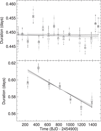
Figure 1. Transit durations and 1-σ uncertainties for planet b (top) and planet c (bottom) found by fitting the long-cadence data. The durations are measured using four different polynomial detrending lengths as described in the text from black to light gray: 7200 minutes (diamonds), 2880 minutes (triangles), 1440 minutes (squares), and 1000 minutes (x symbols). There is minimal variation among the different timescales, so we conclude that our choice of 1 day (1440 minute) detrending is justified. A clear trend appears in planet c.
Download figure:
Standard image High-resolution image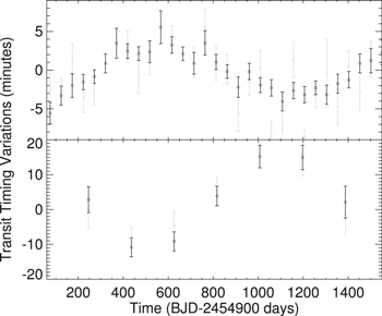
Figure 2. Individually measured TTVs with 1-σ uncertainties (gray). Plotted in black are the mean and variance for TTVs measured by taking 100 random draws from the posterior of photodynamical fit as described in Section 3. Therefore the black points combine the Kepler observational data with a physically possible N-body gravitational model to better constrain the TTVs.
Download figure:
Standard image High-resolution imageWe note that the TTV super-period,  , may be predicted analytically:
  days, where
  is the distance from the 4:1 resonance for planets b and c in our case (Lithwick et al. 2012). This agrees very well with the observed TTV data (Figure 2). On the other hand we may also consider the affects of stellar variability, particularly spots, on the measured TTVs and TDVs. Star spots are darker than the surrounding areas on the face of the star. Thus planet transits which cross a star spot may bias the measured transit time or duration. Crossing star spots in the first half of the transit may cause the transit center time to appear later than the actual time and crossing spots in the second half may cause the transit to appear earlier than it actually occurs (see Holczer et al. 2015). Such an effect is generally small, but we consider them here. In order to reproduce the long-period sinusoidal TTVs present in the planets, the spots would have to be in nearly the same location for successive transits, only slowly moving over the course of the four-year observing window. This implies that it is merely a coincidence that
  is well-matched by the data, and the observed TTVs are caused by a near-commensurability of the planets’ orbital periods with the stellar rotation period or a multiple of it. This does not make physical sense because the period ratios of the two planets have nearly a 4:1 commensurability yet their TTVs are anti-correlated, even in places where they transit very closely in time (e.g.,
  ), indicating the effect of spots is small compared to the implied gravitational TTV effects. Durations may be similarly affected by star spot crossing, but we would predict that any star spots that would make ingress appear later or egress appear earlier would both cause the duration to decrease. For the duration to experience a net decrease as observed, it would require an increase in the number of spots as a function of time over the observing window regardless of location, but no signs of this are seen in the TTVs. We would expect the durations to decrease when the TTVs are greatest in absolute value if caused by star spots, and this correlation is not observed in the data. Thus we rule out star spots as causing the observed TTV and TDV variations.
2.2. Analysis of Stellar Properties
An asteroseismology study conducted by Huber et al. (2013a) found Kepler-108's mass to be  . However, Kepler-108 has been the subject of several follow-up studies which have revealed that it is a binary star system. Adaptive optics (AO) measurements in the i (Law et al. 2014), J, and K bands (Wang et al. 2015) have revealed a companion star 1
05 from Kepler-108A, which is highly likely to be associated with the system (Wang et al. 2015). The binary nature of the star system is also seen in archival UKIRT images (Lawrence et al. 2007).
To determine which star is the planet host, we examine the Kepler pixel level data and the Data Validation Report (DVR) (Bryson et al. 2013). Kepler's pixels are approximately 4″ and thus the two sources are not resolved, but we may still determine where within a given pixel a planet’s host star lies. Because the field is crowded (including by KIC 9471979, a star within one apparent magnitude of the target stars, located approximately 10 arcsec to the south and 3 arcsec to the east), detecting the centroid shift while the planets are in and out of transit, is not effective at determining which member of the binary the planets are transiting because the centroid is affected by these bright stars that are somewhat further away (Bryson et al. 2013). Finding the centroid of the flux difference image (the difference in flux between when the planets are in and out of transit) should reveal the true location of the star being transited, though this method is potentially more uncertain. The DVR indicates that the host star of both planets b and c is approximately 0.5 arcsec east and 0.15 arcsec south of the nominal KIC location at the 4.6-σ and 2.2-σ levels for each planet respectively. Since the KIC location reflects the combined light of the binary star, its reported position is in between the two observed stars (with the fainter, planet-hosting star lying to the southeast). This is confirmed by centroid fitting of the UKIRT J-band images with find.pro and starfinder.pro (Diolaiti et al. 2000) and explains why the centroid offset is only ∼0.5 arcsec, rather than the 1.05 arcsec separation reported by AO imaging (Law et al. 2014; Wang et al. 2015). We find that stars A and B are located at approximately ( ) and
) and  respectively, whereas the DVR indicates the star hosting planets b and c is located at (
 =
= ) and (
 =
=  ) respectively. Thus the planets are consistent with each other and Kepler-108B, but not Kepler-108A. The position angles (PAs) from the KIC location of the host star of planets b and c are
  and
and  respectively, matching the reported PA of the fainter binary companion of 118° in both AO images, and 180° from what would be expected from the brighter star. In summary, this analysis reveals that the position of the planets’ host star is consistent with the southeastern star of the binary pair (Kepler-108B), and rules out the brighter star to the northwest (Kepler-108A) at
  .
.
We use the publicly available Dartmouth stellar isochrone modeling package isochrones (Morton 2015, available at: https://github.com/timothydmorton/isochrones) to characterize the stars based on the AO flux measurements. We have apparent system magnitudes (taken from https://cfop.ipac.caltech.edu) and the magnitude differences between the two stars in the i, J, and K bands (Table 1). Based on these, we compute the magnitudes of both Kepler-108 stars to use as input parameters to the isochrones package. We find that stellar parameters from the AO color constraints are consistent within 1-σ of the asteroseismology for the brighter star Kepler-108A (the non-planet hosting star); however the isochrone method has uncertainties a factor of a few greater than asteroseismology. Lower accuracy is expected from the photometric method because asteroseismology is one of the most precise methods of determining stellar density, and thus masses and radii combined with stellar models, developed to date. Nonetheless, the agreement between the different methods of estimations confirms that photometry can determine the properties of the planet host star, albeit with large uncertainties. We suggest therefore that our results be interpreted more as broad priors on the scale of the system and stellar density rather than a precise stellar measurement. We summarize our inputs and fitted values in Table 1 and find that the planet-hosting star has  and
and  .
.
Table 1. Kepler-108 Stellar Properties
| Kepler-108 A | Kepler-108 B (Planet Host) | |
|---|---|---|
| Asteroseismologya | ||

|
1.377 ± 0.089 | ⋯ |

|
2.192 ± 0.121 | ⋯ |
| Photometry | ||
 b
b
|
12.654 (Both Stars Combined) | |
 c,d
c,d
|
12.90 ± 0.22 | 13.77 ± 0.22 |
 c,e
c,e
|
12.087 ± 0.15 | 12.287 ± 0.15 |
 c,e
c,e
|
11.640 ± 0.15 | 11.840 ± 0.15 |
 f
f
|

|

|
 f
f
|

|

|
Notes.
aHuber et al. (2013a). bKIC Catalog. c https://cfop.ipac.caltech.edu. dLaw et al. (2014). eWang et al. (2015). fMorton (2015).Download table as: ASCIITypeset image
2.3. Photodynamic Analysis
We followed up our initial analysis of Kepler-108 by applying a photodynamic model. The model integrates the three-body Newtonian equations of motions for the central star and two planets, including the light-travel-time effect. When the planets pass between the star and the line of sight, a synthetic light curve is generated (Pál 2012), which can then be compared to the data. For computational efficiency, we assume that the planets’ velocities are changing negligibly over the face of the host star due to eccentricity effects. By neglecting the change in planet velocity, this approximation ignores asymmetries in the ingress and egress that are on the order of  s, translating to errors in the normalized light curve of only ≲10−6 (see, e.g., Winn 2010, pp. 55–77), much less than the uncertainty on the data. For the photodynamics, we took advantage of the short-cadence (58.8 s exposure) data available in Kepler quarters 5–8 and 12. CBVs are not available for short-cadence data. To detrend this data, first we masked out the expected transit times and then fit a cubic polynomial model with a 1 day width (as done for the long-cadence data) centered within half an hour of each data-point, to determine its baseline. We divided the flux by this baseline. We continued using long-cadence data where short cadence was not available (Kepler quarters 1–3, 9–11, and 13–17). We detrended that data identically as described above for the short-cadence data. We performed detrending with and without using the CBVs and found statistically negligable difference in the fitting results. We used the photodynamic model to produce theoretical normalized flux values at the timestamp of each short-cadence data point. For long-cadence data, we computed the flux value at 15 equally spaced points in time over a cadence’s integration and averaged them together to produce the theoretical result. A small amount of correlated noise (fractional variations
  , with a peak in a Lomb–Scargle periodgram of the out-of-transit short-cadence data near 45 minutes) was still present in the data likely due to known spurious instrumental frequencies (García et al. 2011; Christiansen et al. 2013) and, more broadly, the stellar variability which allowed for asteroseismology measurements. Our detrending algorithm did not address this short-timescale noise to avoid distorting the transit shapes, but its amplitude is far below the data uncertainties. We multiplied the quoted data uncertainties by a factor of 1.075 such that the reduced
  of our best-fitting model was 1.0.3
By increasing our uncertainties, we conservatively widen our posteriors to take into account the scatter introduced by unmodeled aspects of the system, such as star spots or instrumental noise, whose affects may be small but non-zero and bias our results. One of the planets, Kepler-108b, had only partial transits observed at ∼BJD 2455959, 2456106, and 2456204 due to pauses in data collection. Our detrending algorithm performs poorly on cases where there is not a baseline on both sides of the transit. Therefore the data within 1 day of these transits was removed from the fits to avoid incorrectly influencing the fit by changing the measured depths. Since the mid-time and duration measurements of these transits is highly uncertain due to having only either the ingress or egress, retaining them would add minimal information to our fits. To expedite the computation, we fit only data within 1 day from any transit, because the model of data far from transit is always a constant: the transit parameters do not affect it. In total we were left with 25,425 photometric data points.
of our best-fitting model was 1.0.3
By increasing our uncertainties, we conservatively widen our posteriors to take into account the scatter introduced by unmodeled aspects of the system, such as star spots or instrumental noise, whose affects may be small but non-zero and bias our results. One of the planets, Kepler-108b, had only partial transits observed at ∼BJD 2455959, 2456106, and 2456204 due to pauses in data collection. Our detrending algorithm performs poorly on cases where there is not a baseline on both sides of the transit. Therefore the data within 1 day of these transits was removed from the fits to avoid incorrectly influencing the fit by changing the measured depths. Since the mid-time and duration measurements of these transits is highly uncertain due to having only either the ingress or egress, retaining them would add minimal information to our fits. To expedite the computation, we fit only data within 1 day from any transit, because the model of data far from transit is always a constant: the transit parameters do not affect it. In total we were left with 25,425 photometric data points.
The parameters for each planet in the differential evolution Markov chain Monte Carlo (DEMCMC, Ter Braak 2005) fit are  , where P is the period, T0 is the mid-transit time, e is the eccentricity, ω is the argument of periapse, i is inclination, Ω is nodal angle, and R and M are radius and mass respectively (with subscripts
  for the planets and ⋆ for the star). The star had five additional parameters:
  , where
  are the two quadratic limb-darkening coefficients and dilute is the amount of dilution from other nearby sources. We use flat priors in all parameters unless otherwise stated below, including uniform priors on
  and
and  , resulting in a flat prior in total e.
The relative flux from each star in the Kepler bandpass is uncertain, so we allowed the fractional amount of flux from the non-host star to vary as a free parameter. We ran photodynamic fits assuming Kepler-108B is the host with the the stellar mass fixed at the value found as described in Section 2.2 because photometry alone can only determine the stellar density when  . Our DEMCMC fits also used the measured stellar radius and uncertainty (
 ) as a data point along with the Kepler photometry. Since dilute is highly degenerate with the size of the planets (
 ), our planetary radii are significantly more uncertain than previously reported values, which did not take into account contamination from another blended source. The shape of the transit does offer some constraints on the dilution so it is not a completely degenerate parameter. We did not include the companion star in our photodynamic model directly because its great distance (at minimum, the measured sky-projected distance of 327 au, Wang et al. 2015) prevents it from detectably influencing the Kepler-108 planets over the Kepler observing window. We discuss potential long-term effects in Section 6. Although it is disfavored, we also ran a second, nearly identical set of DEMCMCs assuming that the asteroseismologically measured star is the host star, and thus fixed stellar mass at
  and used the constraint
  (Huber et al. 2013a). We include these posteriors in the
To test whether our detection of changing transit durations and depths (and therefore mutual inclination) was robust, we ran three different DEMCMCs for each host star: ( —“Mutually Incline”) allowing the inclinations and relative nodal angle of the planets to vary independently; (
 —“Nearly Coplanar”) allowing only the planets inclinations to vary independently and fixing both planets to a nodal angle of
  and (
and ( —“Coplanar”) forcing the planets to be coplanar, i.e., fixing
  and
and  , but allowing the value of the inclination to vary.
Requiring strict coplanarity ( ) results in a far worse fit to the data (
 ) than the other two models (
 and
and  ) regardless of host star, because each planet must have the same inclination. As a result, the impact parameter of both planets is determined by a single inclination, and the transit shapes and durations of both planets cannot be fit well compared to the case where two different inclination values are allowed. We no longer discuss
  as a viable candidate model since with only one additional free parameter compared to
  we vastly improve the fit and provide a more realistic model.
The  (
( ) DEMCMC was initialized with the periods of the two planets as reported in the Kepler catalog (Batalha et al. 2013), and at a variety of eccentricities below 0.1 for both planets. The DEMCMC chains slowly explored increasingly higher eccentricities, with the chains preferring for the inner planet (b) to have
  . Once the DEMCMC chains found this high-eccentricity space, they did not travel back to lower eccentricities because high eccentricity allowed a better fit to the data. Restarting the DEMCMC from a variety of solutions with planet b having
  and
and  (near the best fit found previously) resulted in none of the chains seeking lower-eccentricity regions. Therefore we conclude that for the nearly coplanar case (
 ), high-eccentricity solutions are robustly preferred. We ran a parallel 46-chain DEMCMC until the parameters appeared stationary; the chains were well mixed (
 autocorrelation timescales for every parameter for each chain on average), and their Rubin–Gellman
  statistic (Brooks & Gelman 1998) was below 1.05 for every parameter. We recorded the parameters for each chain every 1000 generations for 5 × 10⁶ generations to reduce correlation and required disk space, and threw out the first 2 × 10⁵ generations of all chains as a burn-in. We thus obtained 2 × 10⁵ samples of the posterior for each DEMCMC, of which at least
  are completely independent.
The  DEMCMC was initialized similarly to
  , with all eccentricities below 0.1. This DEMCMC also explored higher eccentricities for planet b, but rather than remain high as in
  , eccentricities continually varied between high and low values (
 ). Concerned that this DEMCMC was not finding the same very high-eccentricity parameter space found by
  , we ran
  again but starting from solutions drawn from
  . All chains in this case quickly found lower-eccentricity solutions and did not return to the very high-eccentricity starting conditions. We ran the (
 ) DEMCMC for
  generations, with a 2 × 10⁵ generation burn-in. This DEMCMC was run much longer because the wide range of acceptable eccentricities caused slower convergence. When the DEMCMC was stopped, each parameter had experienced
  autocorrelation timescales (at least 1000 independent points) and had an
  statistic below 1.1. These values are still acceptable for convergence and continuing running was not computationally feasible. The complex nature of the parameter space (see Figures 3 and 4) slows down the convergence significantly, particularly at high eccentricity. DEMCMC runs with Kepler-108A as host have similar statistics.
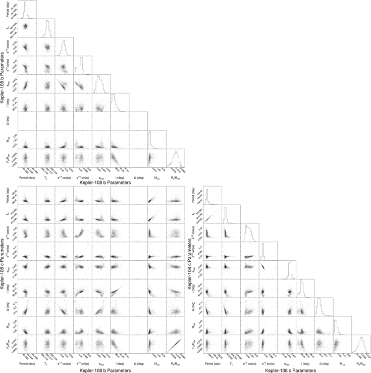
Figure 3. Correlations among all planetary parameters in  , the mutually inclined model. Where correlations would be between a parameter and itself, instead a histogram of the distribution of that parameter is shown.
Download figure:
Standard image High-resolution image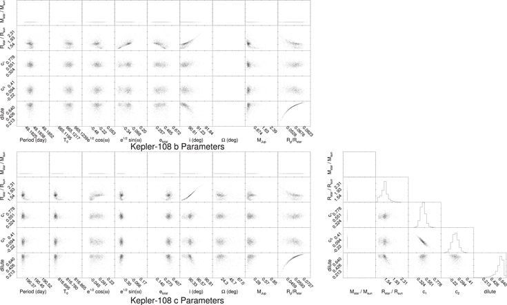
Figure 4. All correlations involving stellar parameters in  , the mutually inclined model. Where correlations would be between a parameter and itself, instead a histogram of the distribution of that parameter is shown.
Download figure:
Standard image High-resolution imageConcerned that we could potentially miss additional minima distant from our initialization on the  surface, we also ran a four-temperature parallel-tempered DEMCMC (Earl & Deem 2005) with both the
  and
and  constraints. This approach is similar to a traditional DEMCMC, but it allows some chains (those with high temperatures) to have a much higher probability chance of exploring high-
 regions of parameter space, allowing them to easily traverse local maxima. This is accomplished by multiplying the
  between a proposed step and the chain’s current location by a given “temperature” value, which increases the probability that higher-
 proposals are accepted. We initialized this DEMCMC from our best-fit solutions, but the high-temperature chains rapidly spread out over a much broader range of parameter space than explored before. The high-temperature chains may swap with low-temperature chains once near a sufficiently low
  minimum and allow for a more refined exploration of parameter space in that area. This allows for efficient discovery and exploration of multimodal posteriors (for further discussion, see Earl & Deem 2005). We find very similar posteriors and no additional minima which would affect our fits with this method.
3. PHOTODYNAMIC RESULTS
The data generally allow for two classes of solutions which cause the observed duration and depth changes in the transits (see Figure 5). The first case, explored by  , we will describe as the low-eccentricity, high mutual inclination case. The second case, explored by
  , refers to the nearly coplanar, highly eccentric case. In this case, the mutual inclination between the planets is
  . The very large (∼0.75) eccentricity of the inner planet along with its increased mass causes faster precession of the node (and apse) of the outer planet. Along with the larger eccentricity of the outer planet, this results in similar transit duration and depth changes (see Figure 6). DEMCMC posterior median values and 1-σ and 2-σ uncertainties at
  (BJD-2454900) for the mutually inclined (
 ) and nearly coplanar (
 ) models are given in Table 2. Note that the distributions in many parameters are not Gaussian and the 2-σ interval is generally not twice as wide as the 1-σ interval. The distributions and correlations between parameters for
  are shown in Figures 3 and 4. Correlations in other fits are similar. Confidence intervals higher than 2-σ are not given as the number of independent parameter values mean that there are relatively large fractional uncertainties on the confidence intervals of higher σ; however, the two sets of confidence intervals given are sufficient to understand the posteriors. Best-fit solutions found by DEMCMC under
  (first) and
  (second) constraints assuming Kepler-108B as the host star at
  (BJD-2454900) are given in Table 3.
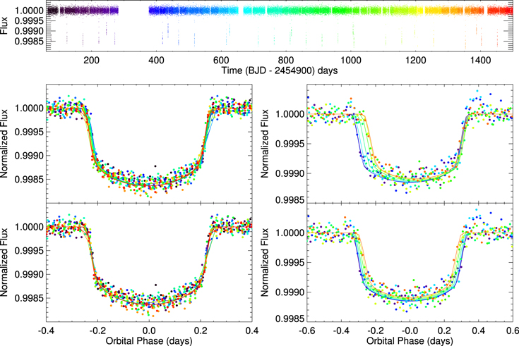
Figure 5. Top: detrended flux over the Kepler observing window. The two planet transits appear clearly as periodic dips of different depth. Color is changed incrementally from violet to red such that each transit has a distinct color in the data. To reduce visual scatter, only long-cadence data are displayed although short-cadence data were used where available in the fitting procedure. Bottom: left and right columns are planets b and c respectively. The top panel shows the data (dots) and photodynamic best-fit model (line) phase-folded with a constant period (the best fit at  (BJD-2454900), see Table 3). Bottom panels show the transits phase folded with the TTVs removed. This allows clear identification of the change in planet c’s duration and depth with time (as indicated by color in the top panel). Model points are produced only where real data points are found and are connected by straight lines resulting in the apparent sharp corners on some of the transits.
Download figure:
Standard image High-resolution image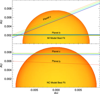
Figure 6. Chords of successive transits of the two planets over the face of the star using the same color scheme as in Figure 5. Top: the favored, mutually inclined ( ) case. Bottom: the disfavored, nearly coplanar (
 ) case. The physical distance the planets in this latter configuration can move across the face of the star is small, so planet c requires a high impact parameter to exhibit large duration changes. The stellar radius increase to ensure the transit duration is correct, and the difference in the ingress and egress shape due to these factors helps distinguish the two models.
Download figure:
Standard image High-resolution imageTable 2. Kepler-108 Posteriors
| Host: Kepler-108B | ||||||
|---|---|---|---|---|---|---|
 —Mutually Inclined —Mutually Inclined |
 —Nearly Coplanar —Nearly Coplanar |
|||||
| Median | 68.3% (1-σ) | 95.4% (2-σ) | Median | 68.3% (1-σ) | 95.4% (2-σ) | |
| Parameter Name (Unit) | Uncertainties | Uncertainties | Uncertainties | Uncertainties | ||
| Stellar Parameters: | ||||||

|
1.57 |

|

|
1.939 |

|

|

|
0.96 | a | 0.96 | a | ||
| c1 | 0.503 |

|

|
0.54 |

|

|
| c2 | 0.01 |

|

|
0.02 |

|

|
| dilute | 0.699 |

|

|
0.22 |

|

|
| Kepler-108 b Parameters: | ||||||
| P (day) | 49.18341 |

|

|
49.18356 |

|

|
| T0 (BJD-2454900 (day)) | 665.12253 |

|

|
665.1095 |

|

|

|
−0.258 |

|

|
−0.758 |

|

|

|
−0.196 |

|

|
−0.483 |

|

|
| eb | 0.135 |

|

|
0.810 |

|

|
| i (°) | 90.42 |

|

|
91.96 |

|

|
| Ω (°) | 0.0 | 0.0 | ||||
M ( ) ) |
0.44 |

|

|
1.39 |

|

|

|
0.0678 |

|

|
0.0439 |

|

|
| Kepler-108 c Parameters: | ||||||
| P (day) | 190.353 |

|

|
190.540 |

|

|
| T0 (BJD-2454900 (day)) | 816.676 |

|

|
816.835 |

|

|

|
0.047 |

|

|
−0.2411 |

|

|

|
−0.347 |

|

|
−0.4528 |

|

|
| eb | 0.128 |

|

|
0.2631 |

|

|
| i(°) | 90.379 |

|

|
90.557 |

|

|
| Ω (°) | 24 |

|

|
0.0 | ||
M ( ) ) |
0.169 |

|

|
0.0202 |

|

|

|
0.05946 |

|

|
0.0398 |

|

|
Notes.
aNote that the stellar mass is held fixed in these simulations so the values and uncertainties on the planets’ masses may easily be scaled with future measurements of the stellar mass. be is not actually a fitted parameter, rather it is derived from and
and  .
.
Download table as: ASCIITypeset image
Table 3.
Kepler-108B Best-fit Solutions (Top:  ; Bottom:
  )
)
| Planet | Period (day) | T0 (BJD-2454900) | e | i (°) | Ω (°) | ω (°) | Mass ( ) ) |
Radius ( ) ) |
|---|---|---|---|---|---|---|---|---|
| b | 49.183083085839172 | 665.122619366413346 | 0.080502815440656 | 90.447992776533482 | 0.0 | −151.443327788289849 | 0.413341841865039 | 0.067139110107278 |
| c | 190.353737335237525 | 816.676288054934048 | 0.135150900332772 | 90.402707451208229 | 21.230171600736064 | −74.804240921039195 | 0.202792331316081 | 0.059698074950235 |
| Stellar Parameters: |
 ( ( ): 0.96 ): 0.96 |
 ( ( ): ): |
1.60826681434233 | c1: 0.519093256451504 | c2: −0.021614974187020 | dilute: | 0.692460493291417 | |
| b | 49.183505940179316 | 665.111210027200173 | 0.800786833080398 | 91.960040412229276 | 0.0 | −147.461456894507307 | 1.494038810020510 | 0.042211249374808 |
| c | 190.557066614127535 | 816.849801840698206 | 0.260953132882452 | 90.557754765511007 | 0.0 | −117.953198816245759 | 0.022840632640538 | 0.038215416346983 |
| Stellar Parameters: |
 ( ( ): 0.96 ): 0.96 |
 ( ( ): ): |
1.942786847021155 | c1: 0.520024994427787 | c2: 0.056552930588019 | dilute: | 0.155848582719487 | |
Download table as: ASCIITypeset image
In a random sample of 100 draws from each posterior distribution, 99% were stable for  years in
  and 100% were stable over the same time period in
  , so stability alone cannot easily rule out either regime.
The fixed nodal angle solution ( ) around Kepler-108B had a best-fit
  for 25,425 data points, and the system allowing non-zero mutual nodal angles (
 ) had
) had  . Since only 1 additional free parameter is added from the
  to
to  models, we would expect an improvement of
  of order unity if both models describe the data well, i.e., if it were true that large mutual inclination was not required to fit the data effectively (Akaike 1974). The large difference in
  suggests that the fit allowing large mutual inclinations is superior to the others by
  as follows.
Rigorously, we can define the F-ratio as the improvement in  normalized by the number of new free parameters, DOF:

to the final reduced  :
:

The F-test gives the probability (p-value) that the F-ratio is as high as observed by chance. In our case the p-value is 1 × 10⁻⁷, so we may reject that the planets have the same nodal angle on the sky. We note that the  being slightly below 1.0 suggests we have overestimated our uncertainties and therefore only strengthens our reasoning.
To compare the entire distribution of parameters found by MCMC rather than just the best-fit solution, we computed the Bayes factor, K, using Newton and Raftery’s p4 estimator (Newton & Raftery 1994) and found the odds ratio to be  in favor of
  , i.e., large mutual inclination is strongly favored (Kass & Raftery 1995).
Lastly, a physical argument can be made in support of  . The radii of the two planets of Kepler-108 differ by only ∼20% (in all scenarios). In the
  model, the planet masses differ by a significant, but reasonable, factor of ∼3. In the
  model, the masses must differ by a factor ∼70, implying that planet c, with a radius
  has a mass of only
  , which implies a lower density than all but the most extreme sub-Neptune planets (Masuda 2014).
Here we have compared the coplanar models only for the case where Kepler-108B is the planet host. However, we perform an identical analysis for the case with Kepler-108A as the planet host, and this analysis also favors the mutually inclined case to a similar significance. Thus, even if there is some doubt regarding which star the planets orbit, we may say unambiguously that the planets are mutually inclined.
3.1. Mutual Inclination
The mutual inclination, I, between the orbital planets of two planets b and c is given by

In our case we have defined  and both planets have
  since they are both transiting. This means that the value of
  . Using the MCMC posteriors on the planets i and Ω values, we compute
  , with a 95% confidence interval of [9
6,
 ]. This is a significant departure from the
  mutual inclination expected from a pure disk formation origin.
4. OBSERVATION STATISTICS
Since the planets in this system are precessing due to the high mutual inclination between them, they will eventually change their orientation so dramatically that they no longer transit. This has been observed in circumbinary systems (Kostov et al. 2014; Welsh et al. 2015), but never in a single-star planetary system. Few other known extrasolar systems are likely to exhibit large inclination variations due to self-excitation (Becker & Adams 2016). To investigate the timescale of the precession in this system, we integrate the best-fit solution forward for 105 years (Table 3). We find that both planets periodically precess on and off the star (see Figure 7). From our viewing perspective, this system has two planets transiting 3% of the time, one planet transiting 4% of the time, and no observable transits 93% of the time. The precession timescale,  , is found numerically to be on average ∼5700 years, somewhat longer than an analytic prediction of ∼4100 years using the frequency for Ω and i oscillations found by applying the Laplace–Lagrange secular solution to first order in planet mass and second order in inclination (e.g., Murray & Dermott 1999).
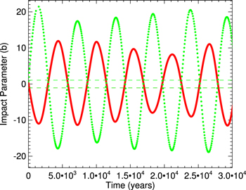
Figure 7. Evolution of the impact parameter (b) of both planets of Kepler-108 over 3 × 10⁴ years. While b is usually reported as a positive definite quantity, we have assigned a negative value for b whenever the position of the planet at minimum b for a given transit is below the center of the star (negative y value). This allows us to visualize the planet moving up and down, on and off the star. Dashed lines show the maximum b where the planet will transit ( ,
,  ). This data are taken from a portion of the 105 year run of the best-fit solution (see Table 3). The asymmetry with respect to b = 0 is due to the invariant plane being inclined to the observer.
Download figure:
Standard image High-resolution imageIn order to better understand the statistics of observing systems like Kepler-108, we explore the likelihood that this system is observed as two transiting planets experiencing TDVs from any orientation. We track the position in three-dimensional space of both planets in our best-fit model every minute for one complete orbit of the outer planet at the beginning and end of the Kepler observing window. That is, we produce two  functions for each planet (
 ,
,  ,
,  , and
, and  ) each 190 days long and
  days apart. We then randomly draw 10,000 different observing orientations and compute the impact parameter (
 ,
,  , k = 1, 2) for each planet (b and c) in both windows (1 and 2) from each orientation. We compute the implied duration (
 ) of the transit corresponding to each
  using (Winn 2010, pp. 55–77):

where the orbital elements come from the instantaneous position and velocity of the planets at the time of minimum b. This is a good approximation for the true duration. The change in duration over the observing window  is given by
  . We establish as a detectability threshold
  minutes (the approximate limit of a confident detection of duration change in Kepler-108) and compute the fraction of observation angles for which
  exceeds the threshold. We use the same threshold for both planets since they are approximately equal in radius, i.e., transit signal.
The results of this analysis are summarized in Table 4 which lists the fraction (and uncertainty) of randomly chosen viewing angles for which the Kepler-108 system would be observable as a two-planet system, one-planet system, and a no-planet system by the Kepler mission. Because the planets are highly mutually inclined, seeing a single-planet transit does not guarantee that the second will be visible. This is seen in the simulations as the two-planet observations are much fewer in number than the one-planet observations, which are dominated by the interior planet due to its closer orbit to the star. The second column shows the fraction of viewing angles for which Kepler-108 would appear to have duration variations in either planet of greater than 30 minutes (a rough limit on a confident detection of the duration change in Kepler-108). Approximately half of the cases where two planets are visible show measurable duration drift; however, in the case where only one planet is visible, measuring a duration drift will happen only ∼18% of the time.
Table 4. Kepler-108 Observational Likelihood
| Fraction of Viewing Angles | Fraction with Planets and a | |
|---|---|---|
| With Planets Observed | Measurable Duration Drift | |
| Two Planets |

|

|
| Single Planet |

|

|
| None Visible |

|
n/a |
Download table as: ASCIITypeset image
It is clear from these statistics that our current viewing geometry is unusual. Since we have observed Kepler-108 as a two-planet system exhibiting TDVs, it is probable that we have also observed similar systems in different viewing configurations. In other words, it is likely that some observed single-Jupiter systems may actually be members of mutually inclined multi-Jupiter systems. Thus, unless we are very unlucky, we expect that a close analysis of many systems with a single transiting Jupiter will reveal duration and depth changes in a few systems due to a non-transiting, mutually inclined companion. However, the measurement of a single planet’s duration change gives very degenerate information about the perturbing planet’s parameters, and it is more challenging to rule out systematics without a well-defined perturbing planet.
5. FUTURE OBSERVATIONS
To assist potential future follow-up measurements, we predict TTVs and 1-σ uncertainties based on 100 random draws from the  posterior up to 10 years after the end of Kepler data collection (Table 5).
Table 5. Kepler-108 Transit Times
| Kepler-108 b | Kepler-108 c | |||
|---|---|---|---|---|
| n | Time (day) | Uncertainty (day) | Time (day) | Uncertainty (day) |
| −12 | 74.908250 | 0.00096 | ⋯ | ⋯ |
| −11 | 124.09378 | 0.00085 | ⋯ | ⋯ |
| −10 | 173.27866 | 0.0010 | ⋯ | ⋯ |
| −9 | 222.46292 | 0.00069 | ⋯ | ⋯ |
| −8 | 271.64736 | 0.00059 | ⋯ | ⋯ |
| −7 | 320.83251 | 0.00085 | ⋯ | ⋯ |
| −6 | 370.01828 | 0.0013 | ⋯ | ⋯ |
| −5 | 419.20153 | 0.00066 | ⋯ | ⋯ |
| −4 | 468.38528 | 0.00061 | ⋯ | ⋯ |
| −3 | 517.56942 | 0.00099 | 245.68312 | 0.0025 |
| −2 | 566.75554 | 0.0014 | 435.99272 | 0.0019 |
| −1 | 615.93794 | 0.00075 | 626.31298 | 0.0019 |
| 0 | 665.12108 | 0.00060 | 816.64113 | 0.0019 |
| 1 | 714.30417 | 0.00098 | 1006.9681 | 0.0022 |
| 2 | 763.49001 | 0.0011 | 1197.2870 | 0.0023 |
| 3 | 812.67222 | 0.00069 | 1387.5972 | 0.0032 |
| 4 | 861.85535 | 0.00061 | 1577.9021 | 0.0059 |
| 5 | 911.03791 | 0.00091 | 1768.2075 | 0.0092 |
| 6 | 960.22324 | 0.00072 | 1958.5204 | 0.010 |
| 7 | 1009.4060 | 0.00068 | 2148.8441 | 0.010 |
| 8 | 1058.5897 | 0.00068 | 2339.1728 | 0.0090 |
| 9 | 1107.7724 | 0.00088 | 2529.4974 | 0.0088 |
| 10 | 1156.9574 | 0.00071 | 2719.8132 | 0.010 |
| 11 | 1206.1410 | 0.00067 | 2910.1212 | 0.012 |
| 12 | 1255.3256 | 0.00065 | 3100.4256 | 0.016 |
| 13 | 1304.5089 | 0.00086 | 3290.7329 | 0.019 |
| 14 | 1353.6939 | 0.00081 | 3481.0495 | 0.020 |
| 15 | 1402.8782 | 0.00069 | 3671.3758 | 0.019 |
| 16 | 1452.0636 | 0.00079 | 3861.7039 | 0.018 |
| 17 | 1501.2478 | 0.0011 | 4052.0257 | 0.018 |
| 18 | 1550.4325 | 0.0011 | 4242.3386 | 0.020 |
| 19 | 1599.6171 | 0.0010 | 4432.6449 | 0.023 |
| 20 | 1648.8026 | 0.0013 | 4622.9495 | 0.027 |
| 21 | 1697.9878 | 0.0017 | 4813.2595 | 0.029 |
| 22 | 1747.1717 | 0.0015 | 5003.5798 | 0.029 |
| 23 | 1796.3560 | 0.0015 | 5193.9076 | 0.028 |
| 24 | 1845.5408 | 0.0018 | ⋯ | ⋯ |
| 25 | 1894.7268 | 0.0022 | ⋯ | ⋯ |
| 26 | 1943.9097 | 0.0018 | ⋯ | ⋯ |
| 27 | 1993.0932 | 0.0017 | ⋯ | ⋯ |
| 28 | 2042.2770 | 0.0019 | ⋯ | ⋯ |
| 29 | 2091.4631 | 0.0022 | ⋯ | ⋯ |
| 30 | 2140.6453 | 0.0017 | ⋯ | ⋯ |
| 31 | 2189.8284 | 0.0016 | ⋯ | ⋯ |
| 32 | 2239.0112 | 0.0017 | ⋯ | ⋯ |
| 33 | 2288.1969 | 0.0018 | ⋯ | ⋯ |
| 34 | 2337.3792 | 0.0015 | ⋯ | ⋯ |
| 35 | 2386.5625 | 0.0015 | ⋯ | ⋯ |
| 36 | 2435.7451 | 0.0015 | ⋯ | ⋯ |
| 37 | 2484.9303 | 0.0015 | ⋯ | ⋯ |
| 38 | 2534.1133 | 0.0014 | ⋯ | ⋯ |
| 39 | 2583.2973 | 0.0015 | ⋯ | ⋯ |
| Kepler-108 b | ||
|---|---|---|
| n | Time (day)a,b | Uncertainty (day) |
| 40 | 2632.4801 | 0.0015 |
| 41 | 2681.6651 | 0.0016 |
| 42 | 2730.8490 | 0.0016 |
| 43 | 2780.0339 | 0.0017 |
| 44 | 2829.2174 | 0.0019 |
| 45 | 2878.4024 | 0.0020 |
| 46 | 2927.5869 | 0.0021 |
| 47 | 2976.7723 | 0.0023 |
| 48 | 3025.9569 | 0.0026 |
| 49 | 3075.1414 | 0.0026 |
| 50 | 3124.3259 | 0.0027 |
| 51 | 3173.5113 | 0.0029 |
| 52 | 3222.6968 | 0.0033 |
| 53 | 3271.8804 | 0.0031 |
| 54 | 3321.0644 | 0.0031 |
| 55 | 3370.2489 | 0.0032 |
| 56 | 3419.4350 | 0.0036 |
| 57 | 3468.6176 | 0.0033 |
| 58 | 3517.8009 | 0.0032 |
| 59 | 3566.9843 | 0.0033 |
| 60 | 3616.1703 | 0.0034 |
| 61 | 3665.3525 | 0.0031 |
| 62 | 3714.5356 | 0.0031 |
| 63 | 3763.7183 | 0.0031 |
| 64 | 3812.9037 | 0.0031 |
| 65 | 3862.0863 | 0.0029 |
| 66 | 3911.2698 | 0.0029 |
| 67 | 3960.4523 | 0.0028 |
| 68 | 4009.6375 | 0.0029 |
| 69 | 4058.8207 | 0.0029 |
| 70 | 4108.0051 | 0.0030 |
| 71 | 4157.1881 | 0.0030 |
| 72 | 4206.3731 | 0.0032 |
| 73 | 4255.5572 | 0.0032 |
| 74 | 4304.7423 | 0.0034 |
| 75 | 4353.9262 | 0.0035 |
| 76 | 4403.1110 | 0.0037 |
| 77 | 4452.2956 | 0.0038 |
| 78 | 4501.4811 | 0.0040 |
| 79 | 4550.6660 | 0.0043 |
| 80 | 4599.8502 | 0.0043 |
| 81 | 4649.0346 | 0.0043 |
| 82 | 4698.2198 | 0.0045 |
| 83 | 4747.4055 | 0.0049 |
| 84 | 4796.5888 | 0.0047 |
| 85 | 4845.7725 | 0.0047 |
| 86 | 4894.9566 | 0.0048 |
| 87 | 4944.1428 | 0.0050 |
| 88 | 4993.3252 | 0.0047 |
| 89 | 5042.5083 | 0.0047 |
| 90 | 5091.6915 | 0.0047 |
| 91 | 5140.8773 | 0.0048 |
Notes.
a(BJD-2454900). bTTVS measured over the duration of the Kepler observing window are set bold while future predicted TTVs are set roman.5.1. Spin–Orbit Alignment
There is limited observable star spot activity on Kepler-108 in the Kepler data due to low S/N. Thus identifying the alignment of the stellar spin with the planets’ orbits was not possible using star spot crossings (Nutzman et al. 2011). Previous spectroscopic measurements of Kepler-108 gave  km s−1 where
  is the inclination of the stellar spin axis to the line of sight and v is the star’s rotational velocity (Huber et al. 2013a). For a star of radius
  , this suggests a maximum rotation period (
 ) of ∼22.4 days, but provides little information regarding the star’s inclination relative to the observer. More importantly, it is not clear for which of the two stars in the binary this measurement is relevant.
The sky-projected angle between the stellar spin axis and the planets’ orbit normals can be measured spectroscopically by identifying the change in apparent radial velocity of the stars as the planet crosses (known as the Rossiter–McLaughlin effect,see, e.g., Gaudi & Winn 2007). The expected Rossiter–McLaughlin amplitude for the observed spin is  m
m  , which is potentially observable (see e.g., Plavchan et al. 2015), though the transits are quite lengthy. These planets likely went through some chaotic destabilization event to get into mutually inclined orbits from their presumably coplanar, protoplanetary disk formation configuration. We therefore predict that the planets could be highly misaligned with the star’s spin-axis.4
5.2. Radial Velocity (RV) Constraints
Although we are confident that this system has a large mutual inclination, a small number of RV data points could help further constrain the system’s parameters. RV measurements may be able to determine which star the planets are truly around and thus refine our fit significantly. Additionally, the RV curves are vastly different in shape between the  and
and  models due to the different eccentricities in the models. If the RV curve is observed to be saw-toothed, it would also give additional constraints on e and ω which are not well-measured in the photometry. Further, because the RV K amplitude is dependent on eccentricity (as well as several other factors, Cumming et al. 1999),

the overall amplitude of the RV signal will be drastically different in the nearly coplanar case  compared to
  , allowing for additional confirmation (Figure 8). In addition, the K amplitude alone will help constrain the value of the mutual inclination in the highly mutually inclined case (
 ) since the K amplitude varies as a function of mutual inclination. A foreseeable challenge for RV measurements is that the two stars are only 1″ apart, roughly the seeing limit for ground-based observations.
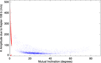
Figure 8. Theoretical K amplitude of the inner planet ( day) as a function of mutual inclination of the two planets for both
  (blue) and
  (red). Plotted are 10,000 randomly chosen points from both posteriors. Not only will a K amplitude give further weight to
  , but it can also be seen that the
  region (
 ) has K dependence, implying RV measurements will better constrain mutual inclination there.
Download figure:
Standard image High-resolution image5.3. Non-transiting Planets
So far our discussion has included only the two planets observed in transit. The TTVs of the two observed planets can, in principle, put constraints on the orbits of non-transiting planets. Since the observed planets have moderate eccentricities and mutual inclinations, we must consider that any unobserved planet also may also have a substantial eccentricity and mutual inclination (which may be the cause of it not transiting). While constraints on non-transiting planets in systems where circular, coplanar orbits are assumed can be quite tight (Agol et al. 2005; Steffen & Agol 2005; Agol & Steffen 2007), considering eccentricity to first or higher orders vastly complicates this process (Agol & Deck 2015). The addition of mutual inclinations will add further allowable TTV frequencies and amplitudes for unseen planets at a given period, and thus decomposing observed signals into the sums of transiting and hypothetical non-transiting planets to set upper limits on unseen planets of a given mass as a function of period becomes untenable.
Since the two planets completely explain the TTVs with the observed Psup matching the expected result from two planets in the observed orbital periods (the residuals are consistent with no signal), we do not appeal to the existence of more planets. Additionally, more planets, particularly in a system of moderately high eccentricities and mutual inclinations, increase the chance that the system would be unstable.
The two known planets in Kepler-108 should both produce observable K amplitudes (planet a:  m s−1, planet b:
  m s−1), and we expect that other Jovian-mass planets in the system with periods shorter than the outermost transiting planet (
 day) may also be detectable through RV measurements. Since we speculate that this system experienced a planet–planet scattering event, it is likely that any other planets in the system may not be coplanar with the observed ones and thus only detectable through RVs, not transits. Small- (
 ) or longer-period (
 day) planets would likely not be detectable by RVs.
6. DYNAMICAL DISCUSSION
We have presented a photodynamic analysis of the orbital parameters of the giant planet system Kepler-108. Planetary systems formed in disks are likely to be coplanar and nearly circular. However, the planets in Kepler-108 are shown to have a high mutually inclination ( ) and eccentricity (
 ), not what one would expect from a purely disk formation origin. Instead, this system shows signs of a more violent, chaotic past as is predicted by theories of secular chaos and the formation of hot Jupiters, establishing an observational link between theoretical stages of planetary system evolution.
The presence of an additional companion star increases the richness of the dynamics of Kepler-108. Kozai–Lidov cycles from a distant companion have been suggested as a means of exciting eccentricities of planets, which may lead to strong planet–planet interactions including scattering and ejection (Malmberg et al. 2007). The timescale for Kozai–Lidov cycles is

(Kiseleva et al. 1998; Fabrycky & Tremaine 2007), where 1 refers to the planet-hosting star, 2 the companion star, p the planet, and  the binary star period. We do not know the period or eccentricity of the outer star, only its sky-projected distance, which is approximately 327 au (Wang et al. 2015). The true distance is likely larger because this measurement ignores the separation of the stars along the axis in the direction of the observer. RV measurements could track the change in velocity as a function of time (i.e., az, where a is the acceleration and the subscript z represents the direction along the line of sight), which would allow an estimate of rz, since M2 and
  are known, where r is the distance between the objects and ⊥ denotes the sky-plane direction, by solving the following for rz:

However, even knowing the true separation of the stars would not reveal the period of the companion star because its orbit may not be circular. Rather, the star may be near pericenter of much larger semimajor axis orbit or near apocenter of a much shorter, highly eccentric orbit. Still, we desire to understand whether or not Kozai–Lidov cycles from interactions with this companion star could be influencing the dynamics of Kepler-108 system.
If we assume the binary orbit is nearly circular and has a semimajor axis approximately equal to the sky-projected distance (327 au), we derive  year and
  . This means that if the inclination of the companion star to the Kepler-108 c is large, it could potentially drive Kozai–Lidov oscillations and cause strong planet–planet interactions on this timescale. It is also entirely possible that the Kozai–Lidov timescale is longer than the age of the system (in large part because the timescale depends on the extremely uncertain
  to the second power), or that the companion star is on a nearly coplanar orbit with the planets, in which case the Kozai–Lidov mechanism does not apply. Additionally, since the planet–planet precession interaction timescale is relatively short
  , this can dominate the dynamics and prevent Kozai–Lidov cycles from occurring. To test this, we run several realizations of the system by integrating forward in time the best-fit solution, with the additional companion star on a circular orbit at 327 au, using the MERCURY integrator (Chambers 2012). We run the simulations for 200 Myr, many times the expected Kozai–Lidov timescale of the system. The inclination of the companion star is varied by 10° intervals from 0° to 180°. To ensure that the Kozai–Lidov mechanism works as expected in a three-body system, we also run the same set of simulations without the inner planet (Kepler-108 b). We find that the planet–planet interactions in the two-planet systems dominate and do not allow Kozai–Lidov eccentricity cycles to occur (see, e.g., Figure 9). All two-planet systems tested remained stable for 2 × 10⁸ years.
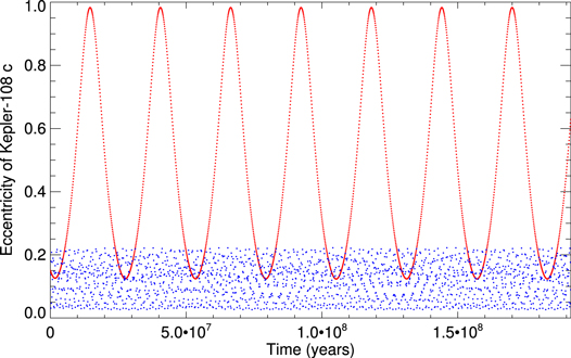
Figure 9. Eccentricity of Kepler-108 c as found by numerical simulation in the presence of a perturbing 1.377  star in a circular 327.5 au orbit and
  . The blue points represent the true two-planet Kepler-108 system. The planet–planet interactions suppress the Kozai–Lidov oscillations and keep Kepler-108 c’s eccentricities at moderate values. Kozai–Lidov oscillations driving Kepler-108 c are clearly present in a simulation with all other parameters identical, but not including the interior planet Kepler-108 b. These points are represented in red and show the very large and potentially destabilizing eccentricity swings that would result in Kepler-108 without taking the strong planet–planet interactions into account.
Download figure:
Standard image High-resolution imageIt is plausible that an additional planet at a much greater orbital period than of the observed two planets could have been subject to Kozai–Lidov oscillations shortly after dissipation of the natal disk, reached a high eccentricity, and caused a planet–planet scattering event. This could result in the large mutual inclination of the two observed planets. However, the parameter space for unobserved, possibly ejected, long-period planets is very large and we do not complete any numerical analysis of this scenario.
The rough similarity between the observed nodal precession timescales and the possible period of the binary star presents another intriguing possibility of the origin of this system: excitation of the planets’ mutual inclination through a Laplace–Lagrange evection resonance (Touma & Sridhar 2015). Studying the Kepler-108 system in this context may require additional data, particularly about the nature of the stellar binary’s orbit, and theory, so we leave it to future work.
7. SUMMARY
We have shown that the two gas giant planets in the Kepler-108 system in 49 and 190 day orbits are mutually inclined. A photodynamic TTV and TDV analysis produces a well-measured precession rate and reveals that a high mutual inclination model ( ) is strongly preferred by the data to a purely high eccentricity case with I less than a few degrees. We compute the likelihood of observing a system similar to Kepler-108 from any orientation and show that the probability of seeing it as a two-planet system with TDVs is very low, suggesting other similar systems exist but have not yet been identified as inclined multiplanet systems.
We thank an anonymous reviewer and Titos Matsakos for helpful comments which greatly improved the quality of this manuscript. We thank Philip Lucas for assistance in understanding the UKIRT data and Thomas Barclay and Jason Rowe for helping us interpret Kepler systematics. This material is based upon work supported by NASA under Grant No. NNX14AB87G issued through the Kepler Participating Scientist Program. D.C.F. received support from the Alfred P. Sloan Foundation. Computer simulations were run using the “Midway” cluster at University of Chicago Research Computing Center. Much of the data presented in this paper were obtained from the Mikulski Archive for Space Telescopes (MAST). STScI is operated by the Association of Universities for Research in Astronomy, Inc., under NASA contract NAS5-26555. Support for MAST for non-HST data is provided by the NASA Office of Space Science via grant NNX13AC07G and by other grants and contracts. The United Kingdom Infrared Telescope (UKIRT) is supported by NASA and operated under an agreement among the University of Hawaii, the University of Arizona, and Lockheed Martin Advanced Technology Center; operations are enabled through the cooperation of the Joint Astronomy Centre of the Science and Technology Facilities Council of the U.K. When the data reported here were acquired, UKIRT was operated by the Joint Astronomy Centre on behalf of the Science and Technology Facilities Council of the U.K. This work makes use of observations from the Las Cumbres Observatory Global Telescope Network, the Kepler Community Follow-up Observing Program (CFOP), and NASA’s Astrophysics Data System (ADS).
APPENDIX: POSTERIORS WITH KEPLER-108A AS THE PLANETARY HOST
We provide system posteriors and best-fit solutions from DEMCMC fits assuming Kepler-108A is the planetary host star in Tables 6 and 7. This is strongly disfavored as discussed in S2.2, but we include the results here for completeness and to demonstrate that the claim of a measured high mutual-inclination between the planets is robust to the choice of host star.
Table 6. Kepler-108 Posteriorsa
| Host: Kepler-108A | ||||||
|---|---|---|---|---|---|---|
 - Mutually Inclined - Mutually Inclined |
 - Nearly Coplanar - Nearly Coplanar |
|||||
| Median | 68.3% (1-σ) | 95.4% (2-σ) | Median | 68.3% (1-σ) | 95.4% (2-σ) | |
| Parameter Name (Unit) | Uncertainties | Uncertainties | Uncertainties | Uncertainties | ||
| Stellar Parameters: | ||||||

|
2.13 |

|

|
2.21 |

|

|

|
1.377 | 1.377 | ||||
| c1 | 0.539 |

|

|
0.541 |

|

|
| c2 | 0.00 |

|

|
0.02 |

|

|
| dilute | 0.42 |

|

|
0.19 |

|

|
| Kepler-108 b Parameters: | ||||||
| P (day) | 49.18336 |

|

|
49.183551 |

|

|
| T0 (BJD-2454900 (day)) | 665.12230 |

|

|
665.1099 |

|

|

|
−0.270 |

|

|
−0.758 |

|

|

|
−0.116 |

|

|
−0.480 |

|

|
| i(°) | 91.06 |

|

|
92.01 |

|

|
| Ω (°) | 0.0 | 0.0 | ||||
| M (MJup) | 0.48 |

|

|
1.93 |

|

|

|
0.0504 |

|

|
0.0431 |

|

|
| Kepler-108 c Parameters: | ||||||
| P (day) | 190.348 |

|

|
190.535 |

|

|
| T0 (BJD-2454900 (day)) | 816.669 |

|

|
816.831 |

|

|

|
0.081 |

|

|
−0.2408 |

|

|

|
−0.353 |

|

|
−0.4516 |

|

|
| i (°) | 90.542 |

|

|
90.567 |

|

|
| Ω (°) | 22 |

|

|
0.0 | ||
| M (Mjup) | 0.193 |

|

|
0.0295 |

|

|

|
0.0449 |

|

|
0.0391 |

|

|
Note.
aThe same as Table 2, except with Kepler-108A as the host star, which is strongly disfavored (Section 2.2).Download table as: ASCIITypeset image
Table 7.
Kepler-108A Best-fit Solutionsa (Top:  ; Bottom:
  )
)
| Planet | Period (day) | T0 (BJD-2454900) | e | i (°) | Ω (°) | ω (°) | Mass (MJup) | Radius ( ) ) |
|---|---|---|---|---|---|---|---|---|
| b | 49.183166276551468 | 665.122980583247113 | 0.089986885710435 | 91.010811057553170 | 0.0 | −154.480618347210282 | 0.431852109916838 | 0.051276491383251 |
| c | 190.351354671141621 | 816.671779290328345 | 0.149122863867700 | 90.522221912212288 | 20.253567886356745 | −78.537503362093275 | 0.177045842528898 | 0.045709799425805 |
| Stellar Parameters: |
 ( ( ): 1.377 ): 1.377 |
 ( ( ): ): |
2.081902708396573 | c1: 0.548773346700056 | c2: -0.020139937332240 | dilute: | 0.440556667838008 | ⋯ |
| b | 49.183540428579263 | 665.111007882649574 | 0.801635029977613 | 91.977223010429583 | 0.0 | −147.861103185700557 | 2.113070778746788 | 0.043754954793284 |
| c | 190.565864464644363 | 816.860367107108004 | 0.260981406054698 | 90.561723018566155 | 0.0 | −118.243316256653287 | 0.029094474876061 | 0.039569609624921 |
| Stellar Parameters: |
 ( ( ): 1.377 ): 1.377 |
 ( ( ): ): |
2.199762169565716 | c1:0.540272159974162 | c2: 0.011661927881225 | dilute: | 0.213472272691092 | ⋯ |
Note.
aThe same as Table 3, except with Kepler-108A as the host star. The values here are 25,409 and 25,432 for the top and bottom parameters respectively.
Download table as: ASCIITypeset image
Footnotes
- 1
However, it is usually difficult to distinguish an inclination of just above
 from just below (both nearly edge-on orbits) with the same impact parameters. In some many-body systems it is possible to distinguish these through either dynamical interactions (Huber et al. 2013b) or overlapping mutual transits (Masuda et al. 2013).
 - 2
There are several known circumbinary systems where the planet is slightly mutually inclined to the binaries and exhibit spectacular precession effects (e.g., Kostov et al. 2014; Welsh et al. 2015), but all seven such currently known systems have low (
) mutual inclinations (Doyle et al. 2011; Orosz et al. 2012b, 2012a; Welsh et al. 2012, 2015; Schwamb et al. 2013; Kostov et al. 2014). Additionally, as such systems are likely to have vastly different histories, here we consider only systems with a single star and multiple planets. - 3
A more careful treatment could, in principle, be done using Gaussian process noise modeling (e.g., Ambikasaran et al. 2014); however this was computationally untenable for our study since we have
data points for a model that needed to be run times to provide posteriors on all of our models. - 4


