Abstract
We study dynamical systems that admit action-angle variables at leading order, which are subject to nearly resonant perturbations. If the frequencies characterizing the unperturbed system are not in resonance, the long-term dynamical evolution may be integrated by orbit-averaging over the high-frequency angles, thereby evolving the orbit-averaged effect of the perturbations. It is well known that such integrators may be constructed via a canonical transformation, which eliminates the high-frequency variables from the orbit-averaged quantities. An example of this algorithm in celestial mechanics is the von Zeipel transformation. However, if the perturbations are inside or close to a resonance, i.e., the frequencies of the unperturbed system are commensurate; these canonical transformations are subject to divergences. We introduce a canonical transformation that eliminates the high-frequency phase variables in the Hamiltonian without encountering divergences. This leads to a well-behaved symplectic integrator. We demonstrate the algorithm through two examples: a resonantly perturbed harmonic oscillator and the gravitational three-body problem in mean motion resonance.
1. Introduction
The Kozai–Lidov mechanism (KL hereafter; Kozai 1962; Lidov 1962), and secular dynamics of triple systems in general, has gained much attention in the past years (see Naoz 2016 for a review). This process describes the secular evolution of a hierarchical triple system due to their gravitational interactions, i.e., how a distant tertiary perturbs the dynamics of a binary on timescales much longer than the orbital periods. Its main feature is the presence of a resonant island in phase space, which corresponds to the libration of the binary’s argument of periapsis g1 (Shevchenko 2017). Hierarchical triples consist of two binaries: the inner binary made up of the tight members and the outer one made up of the tertiary and the barycenter of the inner binary. The KL mechanism drives oscillations in the eccentricities of the inner and outer binaries and their mutual inclination, while the semimajor axes remain constant. In the quadrupole approximation ( ) the system is integrable (a fact that is referred to as a “happy coincidence”; Lidov & Ziglin 1976). The octupole approximation (
 ) is chaotic, which drives the eccentricities to almost unity and inclination flipping, a phenomenon called the eccentric KL mechanism (Katz et al. 2011; Lithwick & Naoz 2011).
The secular equations of motion are derived from the Hamiltonian of the triple system by averaging over the quick angle variables, i.e., the mean anomalies of the inner and outer binaries l1 and l2 (Valtonen & Karttunen 2006). These angles are then cyclic variables in the orbit-averaged effective Hamiltonian, which makes the conjugate momenta constant (i.e.,  , expressed with the semimajor axis), thus the hierarchical three-body problem is stable. Such an elimination of the quick angle variables is carried out by a canonical transformation first applied by von Zeipel (1910). The von Zeipel transformation is based on a generating function that contains both the original and the new variables, which makes the connection between them implicit and difficult to work with when higher-order terms are also taken into account. An alternative derivation utilizes Lie transformations to eliminate the quick angles, giving explicit connections between the original and the new variables (Hori 1966).
However, the orbit-averaged approximation may fail to describe the evolution accurately in many cases (Liu et al. 2015; Luo et al. 2016; Grishin et al. 2018; Liu & Lai 2018; Bhaskar et al. 2021). In this paper we examine the effects of orbital resonances.
Mean motion resonances (MMRs) play a key role in astrophysics including planetary and stellar dynamics. However, secular evolution in such resonances has been identified to be “one of the most complicated topics of Celestial Mechanics” (Morbidelli 2002). The main complication is that the generating functions constructed to eliminate the perturbation from the Hamiltonian have divergent denominators in the case of MMRs. In other words, the averaged equations of motion obtained by the von Zeipel/Lie transformation break down in the resonant case. The standard way to avoid this problem is to transform the Hamiltonian of the system to new variables, where one of the coordinates is the resonant angle (which changes slowly) and the other is to be averaged over. The new Hamiltonian is analogous to that of a pendulum, where the resonant angle either librates around the exact resonance or it rotates (Murray & Dermott 2000). In this way, Sansottera & Libert (2019) reformulate the Laplace–Lagrange theory within MMRs. Another approach was introduced by Wisdom (1982), a numerical method with which the long-term evolution of perturbed bodies in/near resonances can be efficiently followed. Instead of being eliminated, the quick angle variables are changed in such a way that they sum up as a series of Dirac delta functions in the perturbing Hamiltonian. The dynamics is then driven by either the integrable or the delta-function part of the Hamiltonian: both can be calculated much faster, hence the numerical integration takes ∼1000× less CPU time. These ideas were extended to the general N-body problem by Wisdom & Holman (1991).
Keeping the resonant angle in the Hamiltonian results in different equations of motion than the secular ones derived by double-averaging the Hamiltonian. As it is more convenient to solve the same set of equations of motion both in and out of resonances, here we propose a canonical transformation that overcomes the difficulty of small denominators, but contrary to previous studies, we do not use the resonant angle as a canonical variable. Instead, we eliminate the quick angle variables by defining a new set of orbital elements that makes the orbit-averaged dynamical equations valid. As long as the resonant perturbation is small, proportional to some ≪ 1, we demonstrate that the system may be integrated exactly in the transformed variables up to
2 order and show that similar subsequent canonical transformations may extend the accuracy of the integration to arbitrary
n
order. We show that this generates a symplectic integrator for resonant systems.
The paper is structured as follows. In Section 2 we describe the canonical transformation with a general Hamiltonian, where we only assume that the perturbation is small and can be decomposed into a convergent Fourier series. In Section 3 we apply this transformation to the case of coupled harmonic oscillators, and in Section 4 to the case of the gravitational three-body problem. We discuss the limitations of the method in Section 5.
Throughout the paper, we adopt units where the gravitational constant is G = 1.
2. The General Secular Hamiltonian in Resonance
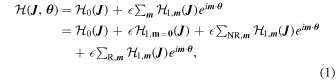
Let us consider an integrable system, the Hamiltonian, which is expressed with its action variables:  . We assume that the system is in resonance or close to it as defined below. Let us also assume that the system is perturbed by a Hamiltonian that can be decomposed into a Fourier series and may be written as
where
J
and
θ
are the action and angle variables (in the absence of perturbations,
J
are adiabatic invariants),  is the unperturbed Hamiltonian, R refers to the resonant terms for which
m
satisfies
m
·
ω
0 = 0, and
is the unperturbed Hamiltonian, R refers to the resonant terms for which
m
satisfies
m
·
ω
0 = 0, and  are the unperturbed frequencies.
  is the angle-independent part of the perturbing Hamiltonian, which drives the evolution of the system on timescales much longer than the period of
θ
(i.e., on secular timescales t ≫ Tk
= 2π/ω0,k
, where k runs through all degrees of freedom). It is obtained by averaging the perturbing part of the Hamiltonian over the angle variables. Physically this procedure amounts to smearing out the orbiting object (e.g., a planet) along its trajectory, which results in a “mass wire”. Technically this is achieved by a canonical transformation for which the transformed momenta contain the effects of the perturbation by definition as we show below. The coupling constant of the perturbation is assumed to satisfy
is the angle-independent part of the perturbing Hamiltonian, which drives the evolution of the system on timescales much longer than the period of
θ
(i.e., on secular timescales t ≫ Tk
= 2π/ω0,k
, where k runs through all degrees of freedom). It is obtained by averaging the perturbing part of the Hamiltonian over the angle variables. Physically this procedure amounts to smearing out the orbiting object (e.g., a planet) along its trajectory, which results in a “mass wire”. Technically this is achieved by a canonical transformation for which the transformed momenta contain the effects of the perturbation by definition as we show below. The coupling constant of the perturbation is assumed to satisfy ≪ 1.
To derive the perturbed secular equations of motion, one has to find a W generating function that eliminates the sums in a way that only the m = 0 perturbation remains in the Hamiltonian. In the first-order approximation this requirement leads to the so-called homological equation:

where [ · , · ] is the Poisson bracket. Its solution is

This famously diverges near MMRs, a phenomenon coined “the problem of small divisors” (Morbidelli 2002). Instead of Equation (3), we propose the following generating functions in order to eliminate the resonant terms (see Sitaram & Mehta (1995) for a similar function):

where k can be any of the coordinates. The final results are independent of which Wk
we use, as we prove below. Equation (4) diverges only when the frequency  , but this does not hold at least for the fastest angle variables in celestial mechanics, which is the subject of this study. The generating function of the inverse transformation is

where  are the transformed canonical variables. In what follows, we restrict attention to two degrees of freedom, i.e.,
θ
= (θ1, θ2),
J
= (J1, J2), to W1, and to the first-order
are the transformed canonical variables. In what follows, we restrict attention to two degrees of freedom, i.e.,
θ
= (θ1, θ2),
J
= (J1, J2), to W1, and to the first-order  approximation. In this case, we can substitute the unperturbed quantities into every term which is already multiplied by
 because the difference between
J
and
 is of order
 (see Equations (22)–(23)).
The canonical transformation and its inverse are generated by W and  for any phase-space component X as


where we introduced the Lie operator

Substituting Equation (5) into Equation (6) yields
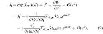
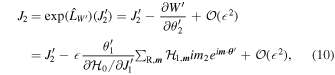


Note that as long as the system is close to a resonance  for which
  such that there exists ∣
ω
i
∣ ≪ 1 and mi
integers and such that initially

in this case the perturbation terms in Equations (9)–(10) may be evaluated at resonance as  because these terms are already multiplied by
 in Equations (9)–(10).
The transformed Hamiltonian is equal to the original one expressed with the transformed variables. Substituting Equations (9)–(10) into the Hamiltonian Equation (1) and Taylor-expanding with respect to , and using the fact that for an arbitrary function F

we get the Hamiltonian in the new variables:
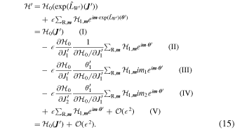
Here rows (I)–(IV) are the transform of  to
to  and row (V) is the perturbation in Equation (1), which transforms trivially as
  and
and  because it is already
  . Rows (II) and (V) trivially cancel each other, while the sum of rows (III) and (IV) vanishes if approaching an MMR:
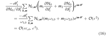
What we are left with is finally

which is independent of  to first order in
 as intended. We note that for the sake of simplicity we omitted the nonresonant sum and the secular term from Equation (1), because the former only induces small oscillations in the actions, while the latter only results in a small frequency shift. The generating function for the case of both resonant and nonresonant terms is the sum of Equations (3) and (4):

Such a transformation eliminates the perturbing terms only to  . Higher-order terms may be eliminated in succession to arbitrary order by applying the same procedure. We demonstrate this through an example in Section 3.
2.1. Initial Conditions
Equations (9) and (10) are seemingly asymmetric (J1 has an extra term as a consequence of the arbitrary choice of θ1 and J1 in Equation (4)), but here we show that the canonical transformation does not have an asymmetry.  and
and  are both constant with only
  corrections and their values are set by the initial conditions: (
θ
,
J
) = (
θ
0,
J
0
). We assume that the resonance is nearly exact initially, i.e.,
corrections and their values are set by the initial conditions: (
θ
,
J
) = (
θ
0,
J
0
). We assume that the resonance is nearly exact initially, i.e.,  . Using Equation (4), the new
  momentum is expressed with the original one as
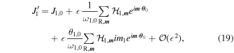
where J1,0 labels the initial value of J1. 3 Now rewrite Equation (9) as
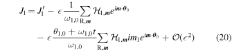
and substitute Equation (20), we get

Doing the same for Equation (10) yields

These expressions for J1 and J2 are symmetric to the reversal of their index despite the asymmetry caused by the extra term in Equation (9) compared to Equation (10). Note that the ignored terms are expected to be small as long as t ≪ 1/(
ωi,0) for all i.
3. Secular Dynamics of Coupled Harmonic Oscillators—A Toy Model
Here we demonstrate the machinery described in the previous section in a very simple case, where two harmonic oscillators with unit frequency are weakly coupled. The Hamiltonian is

where ∣∣ ≪ 1, ∣
ω1∣ ≪ 1, and ∣
ω2∣ ≪ 1. The angle variables are the phases of the oscillations and the actions are
 , where Ak
is the amplitude. The oscillators are weakly coupled as ∣
, where Ak
is the amplitude. The oscillators are weakly coupled as ∣∣ ≪ 1. We note that this system is integrable because it has two first integrals,
 and J1 + J2, whose Poisson bracket vanishes (Masoliver & Ros 2011). The exact solution is derived in Appendix B. This makes it simple to test the error of our algorithm.
The leading-order terms satisfy  , so ωi,0 = 1 +
 ω
i
. This implies that the system is at or close to a 1:1 resonance, respectively, if
ω
i
= 0 or ∣
ω
i
∣ ≪ 1 so the standard recipe for eliminating the perturbation diverges because the perturbing term depends on the difference of the angle variables θ1 − θ2, which results in
m
·
ω
= ω1,0 − ω2,0 =
ω1
ω1,0 −
ω2
ω2,0 approaching zero in the denominator of Equation (3).
3.1. First-order Approximation
First we eliminate the terms proportional to . Let us define the generating function using Equations (4) and (5) with k = 1, which simplify to


where

The canonical transformation formulae between the original and the new variables are given by Equations (9)–(10), i.e.


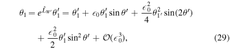

where  .
.
The new Hamiltonian may be obtained by substituting into Equation (24) or by  :
:
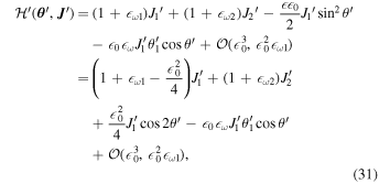
where we introduced the notation

Ignoring the  corrections, the equations of motion of the primed variables are formally the same as the unperturbed/averaged ones:




As the perturbation is second order,  are conserved if ignoring
  perturbations. The
  corrections include both a secular
  and a resonant term
  . The second-order orbit-averaged evolution corresponds to dropping the periodic term; however, this simplification is not necessary as shown in the next subsection. The secular term results in a constant secular shift in the frequency of the first oscillator because
  . The frequencies of the oscillators may change secularly for more general perturbations.
3.2. Second-order Approximation
Let us now proceed to eliminate the remaining perturbation terms  from the Hamiltonian Equation (32) to
 2 order. For
 , the generating function is chosen using Equations (4) and (5), which simplifies to

where  and
and

The new canonical variables are
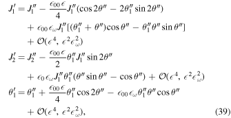

Combining Equations (28)–(31) and Equations (40)–(41) we get
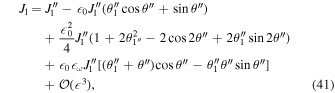



Here and in what follows  denotes
  . The Hamiltonian Equation (24) in these canonical variables is

implying that the system evolves according to



where i ∈ {1, 2} and  are the initial conditions whose values may be obtained from the initial conditions using the inverse transformation
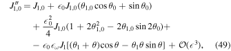



where θ0 = θ1,0 − θ2,0.
Figure 1 shows the time evolution of the J1 momentum for the parameters shown in the figure caption. We compare the exact solution (see Appendix B) with the first- (Equation (28)) and second-order (Equation (42)) solutions. We note that the case of the right panel is remarkably simple. The exact solution is J1 = e−
t
(see Equation (B18)), so the first- and second-order solutions are
 . The first three terms of the J1 Taylor series are recovered correctly with the method introduced in this section.
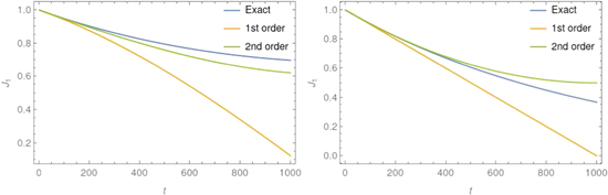
Figure 1. The time evolution of the J1 action for the perturbed harmonic oscillator driven by Equation (24). Initial conditions are (θ1,0, θ2,0, J1,0, J2,0) = (1, 0, 1, 1) for the left panel and (0, 0, 1, 1) for the right. The perturbing parameters in the left and right panels are (,
ω1,
ω2) = (0.001, 0.002, 0.0025) and (0.001, 0, 0), respectively. The orange and green curves show the first-order (Equation (28)) and second-order (Equation (42)) solutions, respectively. The blue curve shows the exact solution (see Appendix B). Note that the unperturbed orbital frequencies are resonant, ω1,0 ≈ ω2,0 ≈ 1, and that the errors are small up to t =
 −1
−1
 −1
1,0.
−1
1,0.
Download figure:
Standard image High-resolution imageThe derivation above may be generalized in a straightforward way to construct higher-order methods. However, we note that the kth-order approximation is valid only if  , i.e., t ≲ 1/
. In order to follow the evolution on longer timescales, the evolution is to be integrated using this method iteratively in steps of
 , where in each step first apply the canonical transformation, Equations (50)–(53), then calculate the time-evolution step Equations (47)–(48) for a Δt time step, and apply the inverse transformation Equations (42)–(45), and finally set the result to be the initial value of the next iteration step. As each iteration is generated by integrating Hamilton’s equations of motion exactly for some Hamiltonian, namely that in which the
  terms are ignored, this integrator is symplectic. Symplectic integrators are advantageous as they conserve phase-space volume and all Poincaré invariants, and their energy errors typically do not grow systematically with time (Binney & Tremaine 2008). Furthermore, the time step may be chosen to be of order 1/
, which may be much larger than the inverse frequency.
4. Secular Dynamics of Gravitational Triple Systems
We investigate the case of the hierarchical three-body problem. Here, hierarchical refers to the small ratio of the separations between the bodies. The potential energy part of the general Hamiltonian for the hierarchical three-body problem is (Valtonen & Karttunen 2006)
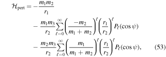
where m1 and m2 are the masses of the inner binary, m3 is that of the tertiary,
r
1 is the separation vector between the members of the inner binary, and
r
2 points from the barycenter of the inner binary to the tertiary.  and r1 ≪ r2 due to the hierarchy.
Now we work out a specific case that is simple enough to illustrate the elimination process introduced in Section 2. We make the following approximations:
- 1.ignore ℓ ≥ 3 multipoles,
- 2.ι = 0, the mutual inclination vanishes, the objects are in the same plane,
- 3.e2 = 0, outer orbit is circular,
- 4.m2 ≪ m3 ≪ m1, the central object is massive and the inner binary has a test particle, which implies that the outer binary’s semimajor axis, a2; eccentricity, e2; and angular frequency, ω2, are constant, and the mean anomaly follows l2 = l2,0 + ω2 t.
With these assumptions, the nonresonant double orbit-averaged Hamiltonian expressed with the Delaunay variables is 4
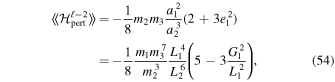
and the secular equations of motion are



where a1 and a2 are the semimajor axes of the inner and outer binaries, respectively, e1 is the inner eccentricity, and

are the conjugate canonical momenta to the mean anomalies l1, l2 and the inner argument of pericenter g1. In order to derive these differential equations, one has to average the Hamiltonian over both the inner and outer orbital motions. Even though Equations (56)–(58) do not have any apparent divergence within MMRs, they originate from a generating function similar to Equation (3) that diverges, suggesting that this may become inaccurate once the inner and outer orbital periods become commensurate.
Here we demonstrate that the divergence of the generating functions in resonance may be eliminated in this problem using the canonical transformation introduced in Section 2. For a proof of concept, we present the algorithm through the 1:2 MMR, although we note that in this case, the triple is not hierarchical. First, Equation (54) can be rephrased as (see Appendix A for the derivation)


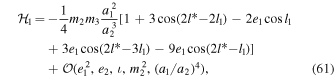
where l* = l2 − g1 and, for the sake of simplicity, we further assume that e1 ≪ 1. 5 At this multipole order, ℓ = 2, we may identify 1:2, 2:3, and 1:1 resonances. However, as we focus on the 1:2 resonance, the other terms can be omitted as long as we are only interested in the terms that systematically grow or decay. In the 1:2 resonance, the 2:3 and 1:1 terms only induce small periodic oscillations in the orbital elements (however, see Luo et al. 2016 for the case when m3 ∼ m1). This simplifying assumption does not restrict generality as the nonresonant terms can be accounted for by utilizing the generating function of Equation (19). The truncated perturbing Hamiltonian then consists of a secular and a 1:2 resonant term:



Note that as the mean anomalies are present only in the 2l* − l1 = 2l2 − 2g1 − l1 combination,

The generating functions analogous to Equations (4) and (5) are

and

where the prime denotes that the function is expressed with the transformed variables. The transformed variables are generated by W as
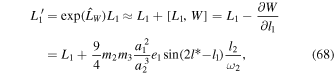
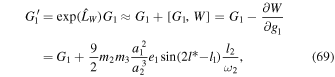
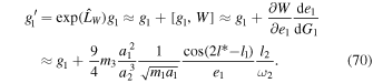
The reverse transformation is very similar, but the change with respect to the primed coordinate has the opposite sign (see Equations (67)–(68)). When transforming Equation (60), the variables in the perturbing Hamiltonian can be simply replaced by their primed counterpart at the quadrupole approximation, as they are already multiplied by the small parameter  (see Equation (14)). The unperturbed Hamiltonian together with the
  truncated perturbations may be obtained as in Equation (15):
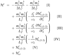
where in the first-order Taylor expansion we used ![${L}_{k}\approx {L}_{k}^{{\prime} }+[{L}_{k}^{{\prime} },W^{\prime} ]={L}_{k}^{{\prime} }-\partial W^{\prime} /\partial {l}_{k}^{{\prime} }$](https://content.cld.iop.org/journals/1538-3881/162/1/22/1/ajabfb6dieqn56.gif) . Using the definition of orbital frequencies
. Using the definition of orbital frequencies

and

and the fact that from Equation (66)  , rows IV and V mutually cancel and the Hamiltonian simplifies as
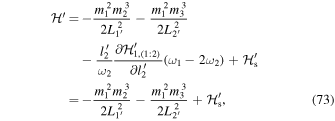
where the term in the parentheses vanishes because of the 1:2 resonant condition. As it is expected,  if
if  . The new equations of motions in the transformed variables are



These equations are orbit-averaged in the sense that the nonresonant oscillating terms have been eliminated from the Hamiltonian. Integrating them gives



These equations are nearly identical to Equations (56)–(58); the only difference is the absence of pericenter precession, which is the result of ignoring the  terms for simplicity. We stress, however, that even though these equations are formally the same, they are derived by a completely different generating function, which avoids divergences in MMRs, and these variables are related to the (a, e, g) orbital elements differently.
Equations (78)–(80) may be expressed with the (a, e, g) orbital elements using Equations (59) and Equations (69)–(71) as



Substituting l2 = l2,0 + ω2
t and setting the  terms properly, it yields that



where the time dependence is also implicit in the variables (l*, l1, e1, a1).
In Figure 2 we plot the evolution of the orbital elements both in the resonant (P1/P2 = 1/2) and in the nonresonant (P1/P2 = 1/2.2) case. The blue and brown curves are the numerical results, while the thick dashed green and orange curves are the fits from the nonresonant and resonant equations, respectively. We observe a qualitative agreement between the direct numerical and the analytical results using the resonant generating function. The discrepancy between the analytical and numerical results is unsurprising. It originates from the approximations we used, especially from the quadrupole assumption. The relative error may be estimated through the ratio of the octupole and the quadrupole terms, which in the 1:2 resonance is

To follow the evolution of the system more accurately on longer timescales, the multipole expansion must be carried out to higher orders, and one must use a smaller time step with an iterative symplectic integration scheme described in Section 3. We leave this to future work.
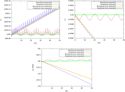
Figure 2. Comparison of the analytical and numerical results within the 1:2 mean motion resonance (blue and orange curves) and slightly out of it (P1/P2 = 1/2.2; brown and green curves). The masses are m1/m2 = 106 and m3/m2 = 10, the semimajor axes are a1 = 1000 and a2=1587.4 (arbitrary units), the inner eccentricity is e1 = 0.05, and the initial mean anomalies are l1,0 = 45°, l2,0 = 0. While the nonresonant analytical solution clearly misses the systematic secular change, the analytical resonant solution is a better approximation. The discrepancy is mostly due to ignoring the octupole and higher multipoles.
Download figure:
Standard image High-resolution image5. Discussion
In this paper we proposed a novel canonical transformation to eliminate the quick angle variables in dynamical systems that admit action-angle variables to leading order and which are subject to resonant perturbations. For a proof of concept, we applied this technique to coupled resonant harmonic oscillators and to the gravitational restricted three-body problem on nearly circular, coplanar orbits in MMR.
This transformation defines a new set of canonical variables explicitly as functions of the orbital elements, in which the perturbed Hamilton’s equations of motion may be integrated trivially. The transformed variables evolve according to the unperturbed equations of motion. Specifically, we have shown that if the perturbations in the original Hamiltonian were of order , the nonintegrable part of the perturbation in the transformed variables becomes ∝
2. We have shown that repeated applications of similar canonical transformations may be used to extend the integrable part to arbitrary accuracy in a series of powers of
. Because Hamilton’s equations may be integrated in the transformed variables with a large time step Δt ∝ 1/
, the iterative application of the canonical transformation, time evolution, and reverse transformation yields an efficient symplectic integrator to simulate the time evolution of the system.
We note that this algorithm cannot be directly applied to systems of three (uneven) degrees of freedom (for example, to Laplace resonances) because resonant terms in the Hamiltonian cancel each other in pairs (see rows III and IV in Equation (15)).
However, for even degrees of freedom, the applicability of this algorithm is not restricted to the simplifying assumptions adopted in the toy models presented here. In the future we plan to further develop this method by (i) relaxing the constraints of the orbital elements to make it applicable for general nonzero inclinations and arbitrary inner and outer eccentricities; (ii) incorporating terms of higher orders in the Hamiltonian, both in (a1/a2) and e; (iii) including general relativistic effects, apsidal precession, and gravitational wave radiation, and exploring Kozai–Lidov oscillations for triple systems that sweep through resonances.
We thank Smadar Naoz, Bálint Érdi, John Magorrian, and Scott Tremaine for helpful comments. We are also grateful to Mária Kolozsvári for help with logistics and administration related to the research. This work received funding from the European Research Council (ERC) under the European Union’s Horizon 2020 research and innovation program under grant agreement No 638435 (GalNUC). B.D. was supported by the ÚNKP-20-3-II New National Excellence Program of the Ministry for Innovation and Technology from the source of the National Research, Development and Innovation Fund.
Appendix A: Derivation of the Resonant Hamiltonian
Here we derive the 1:2 resonant Hamiltonian for the gravitational three-body problem up to quadrupole accuracy.
The cosine of the angle between r 1 and r 2 is

where v1 is the true anomaly of the inner binary and the other notations are the same as before. The argument of the inner periapsis is present only in the combination l* = l2 − g1, so g1 disappears when we average over l* (or l2). This implies that the inner eccentricity (e1) remains constant on the secular timescale. Now we have to express the true anomaly by the mean one, for which we use e ≪ 1 and e2 ≈ 0. In the  approximation the Kepler equation is modified as

where E1 is the eccentric anomaly and from which it follows that


Converting the eccentric anomaly to the true one, we obtain

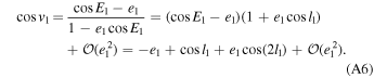
Substituting Equations (A5) and (A6) into Equation (A1) we get
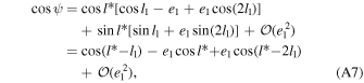
and from Equation (A4)

As the outer orbit is circular, r2 = a2. With all this preparation, the perturbing Hamiltonian in Equation (54) reads (up to quadrupole order and with m2 ≪ m1)
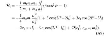
The term that corresponds to the 1:2 MMR is

Appendix B: Exact Solution to the Perturbed Harmonic Oscillator
Here we present the exact solution for the Hamiltonian Equation (24),

and introduce the canonical transformation
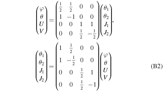
so that

where  and
and ω
=
ω1 −
ω2. Hamilton’s equations of motion are




This shows that U is a constant, and we may integrate the equation for θ and express all other phase-space variables with θ. A trivial solution is the case when  , then θ = θ0 for all times and the equations of motions may be integrated to give
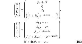
Otherwise we will assume that  . Then
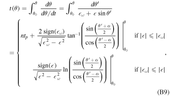
where tp
= t(2π) − t(0), n is an integer, and  if ∣
if ∣∣ ≤ ∣
ω
∣ and
 otherwise if ∣
ω
∣ ≤ ∣
∣. Note that in both cases this may be inverted analytically to give θ(t) in a closed form, but the resulting expression is complicated and we do not show it here. If ∣
∣ ≤ ∣
ω
∣ then, depending on the sign of
ω
, θ either increases or decreases monotonically for all times without bounds,
6
otherwise if ∣
∣ ≥ ∣
ω
∣ then, depending on the sign of
 , θ increases or decreases monotonically such that
  approaches −
ω
/
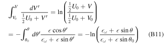
as t → ∞. Now to solve for the evolution of V, divide dV/dt by d
θ/dt

This is a separable differential equation because U is a constant:

Finally, to find the evolution of φ, divide d φ/dt by d θ/dt,
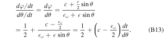
This may be integrated with respect to θ to give

Substituting into Equation (B12) gives the parametric solution in the original variables:
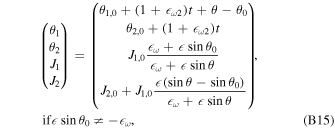
where t(θ) is given by Equation (B19). Note that for ∣ω
∣ > ∣
∣,
 is oscillatory in the full range −1 and 1, and for ∣
ω
∣ ≤ ∣
∣, it changes monotonically, and so J1 and J2 exhibit bounded oscillations and for ∣
ω
∣ ≤ ∣
∣, the denominator asymptotically vanishes so J1/J1,0 → ∞ and J2/J1,0 → − ∞ . For
 , the evolution is given by Equation (B18).
Footnotes
- 3
We note that we can replace
 with ω1,0, because the term including it is already multiplied by
 .
- 4
See Equation (9.30) in Valtonen & Karttunen (2006) with our assumptions.
- 5
We caution that dropping the terms proportional to
might cause trouble. For example, if we ignore it in Equation (55), then the right-hand side of Equation (58) vanishes, hence we miss the pericenter precession. However, as we will show below, the ∼e1 approximation is sufficient to show the effect of the resonance. - 6
However, note that θ ≡ θ + 2n π if n is an integer.

