Abstract
Diffuse radio recombination lines (RRLs) in the Galaxy are possible foregrounds for redshifted 21 cm experiments. We use EDGES drift scans centered at −267 decl. to characterize diffuse RRLs across the southern sky. We find that RRLs averaged over the large antenna beam (72° × 110°) reach minimum amplitudes of R.A. = 2–6 hr. In this region, the Cα absorption amplitude is 33 ± 11 mK (1σ) averaged over 50–87 MHz (27 ≳ z ≳ 15 for the 21 cm line) and increases strongly as frequency decreases. Cβ and Hα lines are consistent with no detection with amplitudes of 13 ± 14 and 12 ± 10 mK (1σ), respectively. At 108–124.5 MHz (z ≈ 11) in the same region, we find no evidence for carbon or hydrogen lines at the noise level of 3.4 mK (1σ). Conservatively assuming that observed lines come broadly from the diffuse interstellar medium, as opposed to a few compact regions, these amplitudes provide upper limits on the intrinsic diffuse lines. The observations support expectations that Galactic RRLs can be neglected as significant foregrounds for a large region of sky until redshifted 21 cm experiments, particularly those targeting cosmic dawn, move beyond the detection phase. We fit models of the spectral dependence of the lines averaged over the large beam of EDGES, which may contain multiple line sources with possible line blending, and find that including degrees of freedom for expected smooth, frequency-dependent deviations from local thermodynamic equilibrium (LTE) is preferred over simple LTE assumptions for Cα and Hα lines. For Cα we estimate departure coefficients 0.79 < bnβn < 4.5 along the inner Galactic plane and 0 < bnβn < 2.3 away from the inner Galactic plane.
Original content from this work may be used under the terms of the Creative Commons Attribution 4.0 licence. Any further distribution of this work must maintain attribution to the author(s) and the title of the work, journal citation and DOI.
1. Introduction
Radio recombination lines (RRLs) have long been a valuable tool used to study the interstellar medium in our Galaxy. These lines appear in the spectra of H i and H ii regions along the plane of the Galaxy (Lockman et al. 1996) and act as a probe of the physical conditions in the regions where they are observed. Line width and integrated optical depth give information about the temperature, electron density, and emission measure of the gas (Salas et al. 2017; Salgado et al. 2017a). Oonk et al. (2017) show that low-frequency carbon and hydrogen lines from molecular clouds can give a lower limit to the cosmic-ray ionization rate. A quantitative study of the low-frequency recombination lines and how they can be used to distinguish hot and cold components of the interstellar medium is done by Shaver (1975a, 1975b).
Diffuse recombination lines not associated with any specific star-forming region are also seen along the Galactic plane and are typically about 0.01%–0.1% of the continuum (Erickson et al. 1995). These lines are usually associated with the colder, lower-density areas inside molecular clouds illuminated by radio-bright objects near the observer's line of sight. Low-frequency carbon line regions are also suggested to be present with photodissociation regions (Kantharia & Anantharamaiah 2001), stimulated emissions from the low-density H ii regions (Pedlar et al. 1978), H i self-absorbing regions (Roshi & Kantharia 2011), CO-dark surface layers of molecular clouds (Oonk et al. 2017), and denser regions within CO-emitting clouds (Roshi et al. 2022). Although helium lines have been observed at 1.4 GHz toward the Galactic center (Heiles et al. 1996) and at 750 MHz toward DR21 (Roshi et al. 2022), due to the lower ionization levels, carbon and hydrogen RRLs are brighter and widely used observables to study the interstellar medium at lower frequencies (Konovalenko 2002). Erickson et al. (1995) used the Parkes 64 m telescope with a beam of ≈4° to survey the inner region of the Galactic plane for carbon RRLs at 76.4 MHz and found a large line-forming region spanning longitudes ∣ℓ∣ < 20° and latitudes within a few degrees of the plane. They also observed numerous targets in the plane of the Galaxy in the frequency range of 44–92 MHz. Cα lines had widths ranging from 5 to 47 km s−1. The region was estimated at distances up to 4 kpc, placing it in the Sagittarius and/or Scutum arms of the Galaxy. They also found lines tangent to the Scutum arm at longitudes between −48° < ℓ < 20° that decreased sharply at ℓ = 20°, believed to be due to change in opacity of the absorbing region. Erickson et al. (1995) suggest that the likely sites for the lines are cold H i regions; however, there were no hydrogen RRL detections.
One of the highly studied regions is around the supernova remnant Cassiopeia A (Cas A). It enables observation of both emission and absorption carbon RRLs (Payne et al. 1989) and is a common target for low-frequency radio telescopes. Oonk et al. (2017) used LOFAR to observe Cas A from 34 to 78 MHz. They found line widths ranging from 5.5 to 18 km s−1, with a line width of 6.27 ± 0.57 km s−1 for C467α. Payne et al. (1989) observed carbon recombination lines in the frequency range 34–325 MHz using the Green Bank Telescope in the direction of Cas A and suggest the origins of the lines to be neutral H i regions in the interstellar medium, which is further supported by the evidence presented in Roshi & Anantharamaiah (1997) using the Ooty Radio Telescope at 328 MHz. Roshi et al. (2002) performed low- and high-resolution surveys of the inner Galaxy over longitudes −28° < ℓ < 89° using the Ooty Radio Telescope at 327 MHz, finding carbon RRLs in emission, primarily for −1° < ℓ < 20°. Kantharia et al. (1998) detect carbon lines toward Cas A at 34.5, 332, 560, and 770 MHz and suggest that the line-forming regions are associated with cold atomic hydrogen in the interstellar medium using the integrated line-to-continuum ratio. Spatially resolved carbon RRLs have also been mapped toward Cas A and used as tracers of the cold interstellar gas (Salas et al. 2018). Carbon RRLs have also been instrumental in evaluating the physical conditions of the line-forming regions around Orion A (Salas et al. 2019).
High-frequency recombination lines are commonly found in dense H ii regions associated with star formation, where the energetic photons ionize the surrounding gas, allowing recombination to occur. This results in RRLs associated with hydrogen, helium, and carbon. Planetary nebulae are another source, as the expanding ionization bubble around protostars and stellar nurseries provide targets for detection. These types of recombination lines have been observed typically above 1 GHz. Using data from the H i Parkes All-Sky Survey at 1.4 GHz to observe H168α, H167α, and H166α RRLs, Alves et al. (2015) mapped the diffuse lines of the inner Galactic plane (−164° < ℓ < 52°) and compared the spatial distribution of the ionized gas with that of carbon monoxide (CO). They reported the first detection of RRLs in the southern ionized lobe of the Galactic center and found helium RRLs in H ii regions, as well as diffuse carbon RRLs. A higher-resolution survey is presented by SIGGMA (Liu et al. 2019) with a beam size of 34 using Arecibo L-band Feed Array in the frequency range of 1225–1525 MHz spanning from H163α to H174α. The project THOR uses the Very Large Array (VLA) to survey H i, OH, and recombination lines from the Milky Way at a resolution of 20″ in the frequency range of 1–2 GHz (Bihr et al. 2015; Wang et al. 2020).
Beyond our Galaxy, extragalactic RRLs have been seen in both emission and absorption. Shaver (1978) used the Westerbork Synthesis Radio Telescope to observe Hα recombination lines in emission from M82. The Expanded Very Large Array (EVLA) detected hydrogen RRLs in emission from NGC 253 (Kepley et al. 2011). More recently, Emig et al. (2019) detected RRLs in the frequency range 109–189.84 MHz in the spectrum of 3C 190 with an FWHM of 31.2 ± 8.3 km s−1 and at a redshift of z = 1.124.
With the advent of experiments aiming to detect redshifted 21 cm signals from neutral gas in the intergalactic medium (IGM) between early galaxies at z > 6, RRLs from our Galaxy and others have been considered as possible foregrounds for the cosmological observations (Peng & Mack 2003). Foregrounds for redshifted 21 cm observations are dominated by Galactic synchrotron radiation, which is typically ∼200 K away from the inner Galactic plane at 150 MHz (Mozdzen et al. 2017; Liu & Shaw 2020; Monsalve et al. 2021), increasing to ∼2000 K at 75 MHz (Mozdzen et al. 2019), and a factor of 10 higher along the inner plane. These levels are 105–106 times larger than the expected 21 cm emission amplitude of 1–10 mK during reionization. Before reionization, some astrophysical scenarios predict 21 cm absorption of ∼100 mK (Furlanetto et al. 2006), and nonstandard physics models can yield 21 cm signals up to 1000 mK (Fialkov et al. 2018). There are strategies in place to mitigate the spectrally smooth foregrounds from observations, including subtraction based on sky models or parameterized fits and avoidance in either Fourier or delay space (e.g., Di Matteo et al. 2002; Bowman et al. 2009; Bernardi et al. 2011; Parsons et al. 2012; Liu et al. 2014; Thyagarajan et al. 2015; Chapman et al. 2016; Kerrigan et al. 2018; Sims & Pober 2019).
Redshifted 21 cm observations aim to study the early epochs of the Universe 6 < z < 200 and target the frequency range of 10–200 MHz. The current generation of instruments primarily aims to make statistical measurements in the epoch of reionization (6 < z < 13, or roughly 100–200 MHz; Fan et al. 2006), where RRLs are typically 0.01%–0.1% of the continuum brightness along the Galactic plane (Erickson et al. 1995; Roshi & Anantharamaiah 1997). Below 200 MHz, RRLs are typically ∼10 K along the plane. This is much weaker than the synchrotron foreground but is still larger than the expected cosmological 21 cm signal. RRLs within this frequency range are therefore important not only for characterizing the diffuse gas regions but also for their effects on 21 cm observations. Hydrogen RRLs are primarily expected to be observed in emission, while carbon RRLs are expected to transition from emission above ∼150 MHz to absorption below (Payne et al. 1989; Erickson et al. 1995). Away from the Galactic center and at high Galactic latitudes where 21 cm observations are generally targeted, RRLs remain poorly quantified (Roshi & Anantharamaiah 2000). If diffuse RRLs away from the Galactic center are about 0.1% of the synchrotron continuum, similar to their ratio near the center, we might expect amplitudes as large as 200 mK at 150 MHz, increasing to 2 K at 75 MHz.
A number of experiments are underway to detect and characterize the redshifted 21 cm signal. They are divided into two groups by observational strategy. The first group attempts to measure the all-sky averaged global signal and includes the Experiment to Detect the Global EoR Signature (EDGES; Bowman et al. 2018), SARAS (Singh et al. 2017), LEDA (Price et al. 2018), and REACH (de Lera Acedo 2019). The second group aims to detect the power spectrum of angular and spectral fluctuations in the signal and includes HERA (DeBoer et al. 2017), LOFAR (Gehlot et al. 2019), OVRO-LWA (Eastwood et al. 2019), and MWA (Tingay et al. 2013). In the 50–200 MHz frequency band of redshifted 21 cm observations, diffuse Galactic RRLs potentially form a “picket fence” with a ≈ 10 kHz wide line every ≈ 300–1900 kHz. The narrow RRLs are easier to mitigate in 21 cm experiments than the brighter, spectrally smooth foregrounds. In global 21 cm observations, the RRL frequencies can be flagged and omitted from signal analysis with little impact on the result (which we will show in Section 4.1). However, for 21 cm power spectrum observations, flagging the RRL frequencies may complicate the analysis by correlating spectral Fourier modes used for the power spectrum estimate. This could potentially spread synchrotron contamination into otherwise foreground-free parts of the power spectrum, even after applying inpainting techniques that aim to fill in missing frequency channels. It would be preferable to skip this flagging if possible.
Here we use observations from the EDGES low-band and mid-band instruments to characterize diffuse RRLs at low radio frequencies. Primarily an instrument designed to measure the redshifted global 21 cm, EDGES also provides an opportunity to study the diffuse RRLs in frequencies relevant to 21 cm measurements during the era of cosmic dawn and epoch of reionization. While the EDGES instruments are very sensitive to faint signals in the radio spectrum between 50 and 200 MHz, they have poor angular resolution. Hence, EDGES observations provide primarily an average line strength over large regions of the sky. We use observed line strengths from EDGES to study the effects of RRLs on global and power spectrum 21 cm observations to determine whether detected RRLs and upper limit levels will have a significant impact on redshifted 21 cm analyses.
In Section 2 we summarize the observations and our methods. In Section 3 we present the results from EDGES low band between 50 and 87 MHz, focusing on the inner Galactic plane in Section 3.2 and away from the inner plane in Section 3.3. We extend the analysis to include 108–124.5 MHz in Section 3.5. In Section 4 we discuss the implications for 21 cm global measurements and 21 cm power spectrum observations, including foreground cleaning. We conclude in Section 5.
2. Methods
EDGES is located at the Murchison Radio-astronomy Observatory in Western Australia. It includes multiple instruments, each spanning a subset of the frequency range between 50 and 200 MHz. Each instrument consists of a wide-band dipole-like single-polarization antenna made from two rectangular metal plates mounted horizontally above a metal ground plane. Below the ground plane sits the receiver, and signals are carried from the antenna to the receiver via a balun.
2.1. Observations
We use 384 days of observations from the EDGES low-band instrument between 2015 October and 2017 April, in the frequency range of 50–100 MHz. The data include and expand on the observations used by Bowman et al. (2018) and Mozdzen et al. (2019). EDGES is a zenith-pointing drift-scan instrument without any steering capability. This gives the instrument a pointing decl. corresponding to the site latitude of −267. At 75 MHz, the antenna beam has an FWHM of 72° parallel to the excitation axis in the north–south direction and 110° perpendicular to the excitation axis (Mahesh et al. 2021). The spectrometer samples antenna voltages at 400 MS s−1 and applies a Blackman–Harris window function and fast Fourier transform to blocks of 65,536 samples to yield spectra with 32,768 channels from 0 to 200 MHz. This results in a frequency channel spacing of 6.1 kHz. Neighboring channels are correlated owing to the window function, yielding an effective spectral resolution of 12.2 kHz.
The size of the EDGES antenna beam is much larger than any single radio source or region. This has two main effects. First, any one source generally will not contribute substantially to the observed antenna temperature. Second, many individual sources or regions may be within the beam at any time, especially along the Galactic plane. The line strengths and line widths observed by EDGES, therefore, will be the aggregate effect of many contributions, each with its own intrinsic broadening and Doppler shift.
The averaging effect of the beam is compounded by the relatively poor spectral resolution of the observations. At 75 MHz, the raw frequency channel spacing of 12.2 kHz yields an equivalent velocity resolution of 48.8 km s−1, which is generally larger than typical gas velocities in RRL regions (see Section 2.3.1). The end result is that these observations are not suitable for studying individual RRL targets in detail, but rather for characterizing the broad RRL properties in different regions of the sky, particularly away from the Galactic center.
2.2. Data Processing
We reduce the EDGES observations and calibrate to an absolute temperature scale following the processes described in Rogers & Bowman (2012), Monsalve et al. (2017b), and Bowman et al. (2018), including filtering of radio frequency interference (RFI). Following this filter, instances of persistent, weak RFI can still be seen in terrestrial FM radio band transmission above 87 MHz. To avoid complications from this interference, we keep only data below 87 MHz for the remainder of the low-band analysis. The data for each day are then binned into 2 hr segments in local sidereal time (LST). Bin centers are referenced to the Galactic center at LST 17.8 hr, yielding a three-dimensional data set in frequency, day, and LST. For simplicity, we refer to the LST bins by their nearest whole hour in the rest of this paper (e.g., using LST 18 hr to refer to the bin centered on the Galactic center) since the distinction is insignificant given the 2 hr width of each bin and large EDGES beam that spans about 6 hr in R.A.
The spectra are fitted with a nine-term polynomial over the frequency range of 50–87 MHz. The expected rms in the daily spectra is typically ∼5 K when the Galactic center is overhead and ∼2 K when the Galactic center is below the horizon. We subtract the fits from the polynomial to obtain residuals that have the continuum removed. We perform RFI filtering again, marking any day-LST bins with residuals larger than 30 K (roughly 6σ) as bad and removing them from the analysis. Typically these cases are due to local weather or abnormal conditions in the upper atmosphere. The resulting total number of spectra for each LST bin varies from 375 to 384. The residuals for all remaining good days within a given LST bin are then averaged to yield a two-dimensional data set in frequency and LST. The duty cycle of the observations was only 17% of wall-clock time, yielding a total of about 126 hr of effective integration time in each LST bin. Figure 1 shows the spectra for LST 18 hr and the corresponding residuals after subtracting a polynomial fit, as well as the expected Cα frequencies. The subtraction of the polynomial fit removes the continuum and other broad structures in the spectra. The residual rms in each spectrum provides an estimate of thermal noise and varies from a high of 374 mK for the spectrum at LST 18 hr, when the Galactic center is overhead, to a low of about 100 mK for LST bins where the plane is primarily near or below the horizon. The noise in each spectrum is strongest at low frequencies because EDGES is sky noise limited and the sky noise follows the synchrotron power-law spectrum.
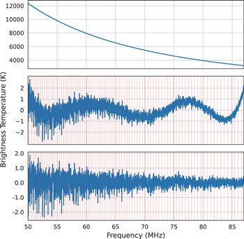
Figure 1. Integrated spectrum (top) and residuals following a five-term polynomial fit subtraction (middle) and a nine-term polynomial fit subtraction (bottom) for the 2 hr bin centered at LST 18 hr, when the Galactic center is at zenith. A five-term polynomial fit fails to capture all the bandpass features, whereas a nine-term polynomial fit removes all the structures, giving continuum-removed residuals. In the middle and bottom panels, the 85 vertical red lines represent the Cα frequencies that are expected within the observed frequency range of 50–87 MHz. Many of the most extreme negative deviations align with RRL frequencies. The lines are strongest at low frequencies, reaching about 2 K below 55 MHz, and weaker at higher frequencies with amplitudes of about 1 K at 60 MHz and less than 0.5 K above 70 MHz.
Download figure:
Standard image High-resolution image2.3. Radio Recombination Lines
When an electron in an atom loses or gains energy, it produces an emission or absorption line based on the change in energy levels. An electron falling from a higher energy state, n2, to a lower energy state, n1, will produce a photon with a frequency (see Gordon & Sorochenko 2009, for details)

where c is the speed of light, R is the Rydberg constant, and Z is the effective nuclear charge seen by the electron (usually very nearly Z = 1 for an excited electron in the outer shell of a neutral atom) for constants in cgs units. The Rydberg constant is given by

where h is Planck's constant, e is the charge of an electron, M is the mass of the nucleus, and me is the mass of the electron.
Free electrons captured by ionized atoms will cascade down through energy levels until they reach the ground state. Transitions are denoted by the element abbreviation, the principal quantum number of the lower energy level (n1), and a Greek letter indicating the change in principal quantum number (n2 – n1) with α = 1, β = 2, etc. Single (α) transitions are the most prevalent and should yield the strongest signals. Within the EDGES low-band range, neighboring α lines for a given species are generally separated by about 300–600 kHz. Cα and Hα lines of the same order are offset from each other by 150 km s−1 in velocity space, with hydrogen lines lower in frequency owing to the lower mass of the hydrogen nucleus compared to carbon. Erickson et al. (1995) observed that β lines are about a factor of two to three weaker than α lines, and γ lines are about a factor of four weaker than α lines at similar frequencies, but this ratio is dependent on specific physical conditions of the gas of any line-forming region. β and γ lines follow similar spacing and offset patterns to α lines in the EDGES band.
2.3.1. Line Widths
The observed line width of a typical RRL is determined by radiation broadening, pressure broadening, and thermal and turbulent Doppler broadening (Roshi et al. 2002; Salas et al. 2017). Only Doppler broadening is significant given the EDGES spectral resolution. The FWHM line width due to Doppler broadening is given by

where ν0 is the center frequency of the line, k is the Boltzmann constant, T is the temperature of the gas, and VT is the turbulent velocity (see Gordon & Sorochenko 2009, for a detailed explanation). For the most extreme case of hot hydrogen gas at T = 7000 K (Oonk et al. 2019), the characteristic thermal velocity is about 11 km s−1. An example H463α line, near the mean effective frequency of 66.1 MHz for α lines in the EDGES band (see Section 2.4), would have ΔνG ≈ 4 kHz in the absence of any turbulent motion. Thermal broadening is nearly a factor of 10 smaller for cold hydrogen gas at T ≈ 100 K. The thermal velocity of cold carbon gas is only about 0.37 km s−1, even lower by an additional factor of 3.5 due to the higher mass of carbon atoms, yielding ΔνG ≈ 0.1 kHz for C463α. Turbulent velocities for motions of individual cells of gas are typically ∣VT ∣ ≈ 20 km s−1 for observations on degree scales (Gordon & Sorochenko 2009). This is generally larger than the thermal velocities and sets a lower bound of ΔνG ≈ 7 kHz for hydrogen and carbon line widths in the EDGES band.
These typical line widths are small compared to the spectral resolution of the EDGES observations. However, the observed lines will include additional Doppler broadening because of other variations in radial velocity between the gas and Earth, including Galactic rotation and Earth's orbit around the Sun. First, when the Galactic center is at the zenith, the large EDGES beam encompasses the broad molecular ring within about ∣ℓ∣ < 30°. The radial velocity for most of the molecular gas in this region sweeps from about −60 to 60 km s−1, increasing linearly with ℓ , although some gas in the inner nuclear disk reaches over 200 km s−1 (Dame et al. 2001). Elsewhere along the plane, the radial velocity of molecular gas is generally within ∣VR
∣ < 40 km s−1. These Galactic rotational contributions are strong compared to the thermal and turbulent contributions to the line width. At 66 MHz, this will contribute about 13 kHz to the line width observed by EDGES when the Galactic center is near the zenith and 7 kHz when other parts of the plane are in the beam. Second, since the data were recorded over 18 months, the projection toward the gas of Earth's ∣VE∣ = 30 km s−1 orbital velocity around the Sun over that period varies. This further broadens line widths in the long integrations. Regions viewed along the ecliptic plane, including the Galactic center and anticenter, are broadened by the full 30 km s−1, equivalent to nearly 7 kHz. The effect decreases away from the ecliptic plane. At a decl. of −267, the effect is weakest around LST 6 hr.
Treating the radial velocity effects analogously to turbulent motions (but neglecting the FWHM conversion factor since they are not necessarily Gaussian distributions) and summing all of the Doppler velocity broadening contributions, the FWHM line widths can be estimated using

For cold carbon gas, the C463α line near the effective frequency of 66 MHz is expected to have width ΔνG ≈ 16 kHz toward the Galactic center and 13 kHz away from the Galactic center. For the hot hydrogen case, the H463α line width toward the Galactic center is about 17.5 and 15 kHz away from the Galactic center. The Doppler-broadened line widths are proportional to frequency and will be about 30% larger at the high end of the observed band. Even with this additional broadening, individual lines are essentially unresolved by the 12 kHz effective resolution of the observations.
2.4. Stacked Profiles
Figure 1 shows the final integrated spectrum from EDGES for the LST 18 hr bin when the Galactic center is at the zenith, as well as the residuals after removing the continuum fit of the spectrum. The RRLs are particularly evident in the residuals below 60 MHz as numerous absorption spikes extending below the noise. An example of an individual line is shown in Figure 2.
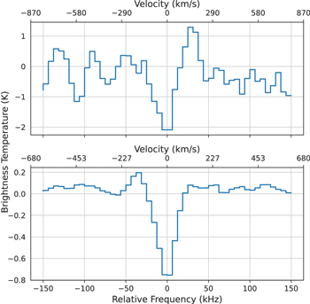
Figure 2. Observed C503α absorption line centered at 51.5 MHz (top) and the stacked average line profile from all 85 RRLs across the band 423 ≤ n ≤ 507 (bottom) for the LST 18 hr bin. The effective frequency of the stacked profile is 66.1 MHz. The significance of detection improves from about 4σ for the individual line to 28σ for the stacked profile.
Download figure:
Standard image High-resolution imageThe thermal noise in the residual spectrum of each LST bin is sufficiently large that individual RRLs are not detected at high significance. We therefore take one additional step to average all of the individual RRLs together within each LST bin. Using the residual spectrum for each LST bin, we extract a window around each expected carbon RRL, centered on the channel that contains the line center. This results in a total of 85 windowed spectra for each LST bin with an effective mean frequency of 66.1 MHz. The effective frequency is below the midpoint of the band because RRLs are more closely spaced at the lower end of the band. Each extracted window spans 300 kHz and contains 49 frequency channels. The full-band polynomial fit subtracted earlier in the analysis removed the continuum background for all lines. The 85 windowed spectra are averaged to yield the stacked profile. The stacking analysis is performed at the data's true spectral resolution of 6.1 kHz, aligning the frequency channels closest to the line centers, resulting in a maximum misalignment in individual lines of 6.1 kHz. Figure 2 illustrates the improvement in signal-to-noise ratio from a single Cα line to the stacked profile for all Cα lines in the band.
3. Results
The stacked α line profiles for each LST bin are shown in Figure 3. In each bin, we see a clear absorption centered on the expected Cα line. In most of the stacked line profiles, we also see a persistent excess in the brightness temperature centered about 35 kHz below the observed absorption line. This emission excess coincides with the expected offset in frequency for the corresponding Hα lines for the same principal quantum numbers, as noted in Section 2.3. We therefore begin in Section 3.1 by simultaneously fitting for Cα absorption-line and Hα emission-line profiles in the stacked spectrum at each LST bin. Then, we proceed to restack the spectra at Cβ and Cγ line centers and fit those lines independently. We note that the noise in the stacked profiles shows non-Gaussian noise that is correlated with the Galactic plane. This could be due to possible narrowband systematics and/or the possible overlapping of some α lines with higher principal quantum number β and γ lines. More sophisticated simultaneous fitting techniques could better address this possibility, but these are beyond the scope of this work.
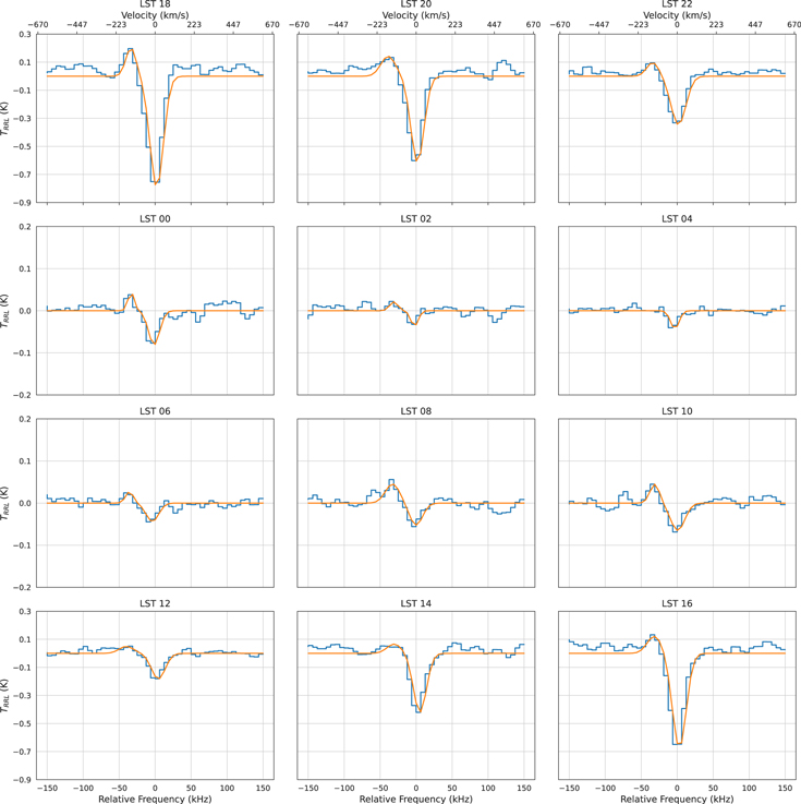
Figure 3. Stacked Cα line profile relative to the continuum for each LST bin (blue) and best-fit double-Gaussian model (orange). Each stacked profile is created from 85 individual lines with principal quantum numbers 423 ≤ n ≤ 507 and has an effective line center of 66.1 MHz. The small emission feature about 35 kHz below the Cα absorption in each panel is from Hα. The lines are strong when the Galactic center is in the beam, peaking at LST 18 hr when the center is at the zenith. They are weak when higher Galactic latitudes are in the beam (e.g., LST 2–6 hr). The best-fit Gaussian profile parameters for each LST bin are listed in Table 1.
Download figure:
Standard image High-resolution image3.1. Observed Line Profiles
The shape of the stacked profile is determined by the line profiles of each of the 85 lines, including their Doppler broadening (about 13–17 kHz), the instrument's spectral resolution (12 kHz), and misalignment of the individual line centers during averaging due to stacking with discrete spectral channels (6 kHz). The first is approximately a Gaussian profile, while the last two are top hat functions. Combining all the broadening contributions results in the effective convolution of a 13–17 kHz distribution with a 12 + 6 = 18 kHz distribution. For cold carbon near the Galactic center, the expected stacked line width is about  . The width is slightly lower when the Galactic plane is out of the beam with
  . Similarly for the hot hydrogen case, the expected stacked line width is about 25 kHz toward the Galactic center and 23 kHz away from the Galactic center. This width is similar to the separation between Cα and Hα lines within the band, which ranges from 25 to 43 kHz with an average of 33.2 kHz. Thus, we expect there to be some line blending between Cα and Hα lines, motivating simultaneous fits of both lines in the stacked profiles to reduce bias and better reflect the uncertainties on the inferred properties.
In each LST bin, we simultaneously fit Gaussian models for the Hα and Cα lines to account for any overlap. The Gaussian model for each line is given by

where A is the peak amplitude of the profile, ν0 is the frequency of the line center, and σ is the standard deviation width of the line. The FWHM of the profile is  . The thermal noise variance used in the fit of the average line profile is derived from the variances for each window. A larger 300-channel region is used to derive these variances, with the lines in each window masked out. The variance is used in the Gaussian fits to estimate the uncertainty on the best-fit parameters. The maximum hydrogen line width is limited by a prior to 24 kHz to prevent the model from trying to absorb any broad structure in the residuals, particularly when the hydrogen line is weak or not present.
The best-fit Gaussian profiles for each LST bin are also shown in Figure 3. Table 1 lists the best-fit parameters. We find Cα line detection significance ranges from 3σ at LST 4 hr, where the best-fit line amplitude is only −33 mK, to 28σ at LST 18 hr, where the amplitude is −795 mK. Hα line detections range from no significant detection at LST 4 hr to 6σ confidence at LST 18 hr, where the line is in emission with amplitude 203 mK.
Table 1. Best-fit Gaussian Model Parameters and Integrated Optical Depths for Each LST Bin
| Bin | Cα | Cβ | Hα | |||||||||
|---|---|---|---|---|---|---|---|---|---|---|---|---|
| LST | A | ν0 | FWHM | τ d ν | A | ν0 | FWHM | τ d ν | A | ν0 | FWHM | τ d ν |
| (hr) | (mK) | (kHz) | (kHz) | (Hz) | (mK) | (kHz) | (kHz) | (Hz) | (mK) | (kHz) | (kHz) | (Hz) |
| 00 | −81 ± 10 | −1 ± 1 | 18 ± 3 | 0.3 ± 0.1 | −8 ± 5 | 10 ± 12 | 64 ± 23 | 0.2 ± 0.1 | 44 ± 15 | −33 ± 2 | 10 ± 4 | −0.1 ± 0.1 |
| 02 | −37 ± 11 | −2 ± 2 | 12 ± 6 | 0.1 ± 0.1 | 0 ± 6 | 10 ± 1 | 47 ± 44 | 0.0 ± 0.1 | 21 ± 10 | −31 ± 3 | 13 ± 12 | −0.1 ± 0.1 |
| 04 | −43 ± 6 | −3 ± 1 | 14 ± 6 | 0.1 ± 0.1 | −10 ± 6 | 10 ± 15 | 44 ± 13 | 0.6 ± 0.4 | 2 ± 1 | −27 ± 24 | 24 ± 57 | −0.0 ± 0.1 |
| 06 | −44 ± 7 | −4 ± 2 | 20 ± 5 | 0.2 ± 0.1 | −32 ± 10 | −5 ± 2 | 13 ± 2 | 0.1 ± 0.1 | 27 ± 8 | −36 ± 2 | 13 ± 7 | −0.1 ± 0.1 |
| 08 | −53 ± 9 | 0 ± 2 | 21 ± 5 | 0.2 ± 0.1 | −43 ± 10 | −5 ± 2 | 21 ± 2 | 0.2 ± 0.1 | 45 ± 9 | −33 ± 3 | 24 ± 7 | −0.2 ± 0.1 |
| 10 | −65 ± 8 | 1 ± 1 | 23 ± 6 | 0.3 ± 0.1 | −37 ± 8 | 0 ± 2 | 23 ± 3 | 0.1 ± 0.1 | 45 ± 13 | −31 ± 2 | 16 ± 5 | −0.1 ± 0.1 |
| 12 | −183 ± 14 | 4 ± 1 | 22 ± 2 | 0.8 ± 0.1 | −84 ± 10 | 5 ± 1 | 16 ± 5 | 0.2 ± 0.1 | 50 ± 27 | −40 ± 3 | 24 ± 7 | −0.2 ± 0.1 |
| 14 | −420 ± 28 | 5 ± 1 | 21 ± 1 | 1.8 ± 0.2 | −162 ± 21 | 5 ± 1 | 23 ± 2 | 0.7 ± 0.1 | 66 ± 18 | −31 ± 5 | 24 ± 9 | −0.3 ± 0.2 |
| 16 | −677 ± 34 | 3 ± 1 | 22 ± 1 | 3.0 ± 0.2 | −304 ± 27 | 4 ± 1 | 25 ± 2 | 1.5 ± 0.2 | 123 ± 34 | −32 ± 4 | 24 ± 7 | −0.6 ± 0.3 |
| 18 | −795 ± 40 | 2 ± 1 | 22 ± 1 | 3.4 ± 0.3 | −261 ± 27 | 2 ± 1 | 29 ± 2 | 1.3 ± 0.2 | 203 ± 46 | −34 ± 2 | 17 ± 2 | −0.7 ± 0.2 |
| 20 | −616 ± 33 | 2 ± 1 | 22 ± 1 | 2.6 ± 0.2 | −211 ± 29 | 3 ± 1 | 26 ± 2 | 1.1 ± 0.2 | 143 ± 32 | −39 ± 3 | 24 ± 5 | −0.6 ± 0.2 |
| 22 | −346 ± 21 | 2 ± 1 | 24 ± 2 | 1.6 ± 0.2 | −162 ± 17 | −1 ± 1 | 26 ± 1 | 0.7 ± 0.1 | 98 ± 23 | −34 ± 1 | 20 ± 5 | −0.4 ± 0.2 |
Note. Integrated optical depths (τ d ν) are calculated using Equation (6). Reported Cα and Hα line profiles have 85 stacked lines 423 ≤ n ≤ 507 with an effective mean frequency of 66.1 MHz, while Cβ has 95 stacked lines 533 ≤ n ≤ 638 with an effective mean frequency of 66.3 MHz.
Download table as: ASCIITypeset image
The typical observed line FWHM is about 23 kHz for Cα and 20 kHz for Hα, in reasonable agreement with expectations. We also report integrated optical depths in Table 1. They are calculated as the area under the best-fit Gaussian model for each stacked absorption-line profile normalized by the observed continuum sky temperature, Tsky, at the effective line center frequency. This is given analytically as

where τ(ν) ≡ ∣TRRL(ν)∣/Tsky(ν). For Cα, the observed integrated optical depths range from 0.1 kHz at LST 2 hr to 3.4 kHz at LST 18 hr. We note that the integrated optical depths are affected by beam dilution (see Section 3.2) if the signal does not fill the full beam.
Figure 4 shows the stacked profiles centered on Cβ lines in each LST bin. Within the same frequency range of 50–87 MHz, we exclude those lines that overlap with Cα within 1 FWHM (n1 = 548, 553, 558, 577, 582, 587, 592, 611, 616, 621, 626) to avoid overlapping of Cα and Cβ lines. We stack 95 Cβ lines with principal quantum numbers spanning 533 ≤ n ≤ 638, resulting in an effective mean frequency of 66.3 MHz. We find that EDGES is sensitive to these lines, with a maximum significance of 13σ for a line amplitude of −304 mK at LST 16 hr. The Cβ profiles drop to the noise level when the Galactic center moves out of the instrument beam. Parameters from these fits are included in Table 1. We do not see clear evidence for Hβ lines, which would be centered about 35 kHz below the Cβ lines, but note additional structures in some LST bins (LST 14 hr, LST 16 hr, LST 18 hr, LST 20 hr) roughly 50 kHz below the Cβ line centers. We rule out RFI as the cause of these, as the structures are correlated with the Galactic plane, possibly indicating unaccounted-for lines or instrumental errors, as discussed above.
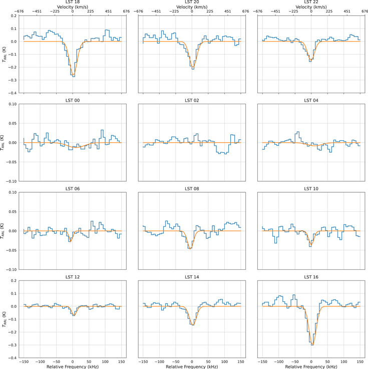
Figure 4. Same as Figure 3, but for C β lines. Each stacked profile is created from 95 individual lines between 533 ≤ n ≤ 638 and has an effective line center of 66.3 MHz. The presence of any contribution from hydrogen is less clear here compared to the α lines; hence, we have fit only a single Gaussian to the main Cβ profile in each bin.
Download figure:
Standard image High-resolution imageFigure 5 shows the stacked profiles at LST 18 hr and LST 6 hr for Cγ lines. We stack 122 Cγ lines with principal quantum numbers spanning 610 ≤ n ≤ 731 at an effective mean frequency of 66.1 MHz. The Gaussian fit to the stacked profile in the LST 18 hr bin gives a 5σ detection of −171.5 ± 34.3 mK. Similar to Cα and Cβ lines, the signal reduces as the Galactic center moves out of the beam. We see no evidence for detection between LST 0 and 6 hr.
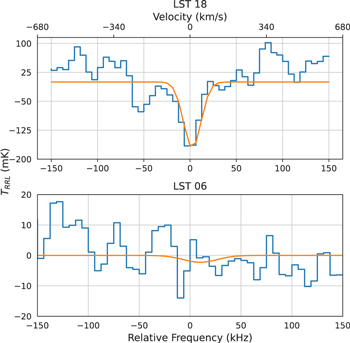
Figure 5. Cγ line profiles, with 122 individual lines stacked, 610 ≤ n ≤ 731, and an effective frequency of 66.1 MHz. The Gaussian model in the top panel gives the best-fit Cγ amplitude of −171.5 ± 34.4 mK when the Galactic plane is in the beam at LST 18 hr, and the bottom panel shows a nondetection when the Galactic plane moves away from the beam at LST 06 hr with a noise level of ∼4 mK.
Download figure:
Standard image High-resolution imageOverall, the magnitudes of Cβ lines are about 30%–50% of the Cα lines at corresponding LSTs and Cγ lines are about 20% of Cα lines, in agreement with trends reported by Erickson et al. (1995). Table 2 gives a summary of all observed line properties at LST 18 hr.
Table 2. Undiluted Line Estimates for LST 18 h
| Line | n | Observed | Undiluted Estimate | |||
|---|---|---|---|---|---|---|
| A | FWHM | A | L/C | τ d ν | ||
| (K) | (kHz) | (K) | (10−4) | (Hz) | ||
| 50–87 MHz | ||||||
| Cα | 423–507 | −0.795 | 22 | −30 | −12 | 9 |
| Cβ | 533–638 | −0.261 | 28 | −10 | −4 | 3 |
| Cγ | 610–731 | −0.171 | 22 | −6 | −2 | 2 |
| Hα | 423–507 | 0.203 | 17 | 7 | 3 | −2 |
| 108–124.5 MHz | ||||||
| Cα | 375–392 | −0.046 | 73 | −2 | −2 | 6 |
| Hα | 375–392 | 0.098 | 49 | 4 | 5 | −8 |
Note. Estimates of line strengths that would be observed by a narrow-beam instrument for the LST 18 hr bin along the inner Galactic plane. The effects of dilution due to the large EDGES beam and long observing season are accounted for.
Download table as: ASCIITypeset image
3.2. Inner Galactic Plane
We begin by comparing the EDGES observations to prior measurements along the inner Galactic plane. At LST 18 hr, when the Galactic center is directly overhead and the primary response of the EDGES beam includes the strong RRL regions seen in previous surveys, the average line profile shows distinct carbon absorption and hydrogen emission lines. The Cα line has a best-fit Gaussian amplitude of A = − 795 mK, and the Hα has a line amplitude of 203 mK. However, we cannot directly compare the amplitudes observed by EDGES to prior observations with higher angular resolution. Due to the large size of the EDGES beam, the inner Galactic plane only fills a relatively small fraction of the total beam. We must account for this beam dilution when the Galactic plane is overhead to compare EDGES observations with prior measurements. The large beam is also responsible for spectral effects not present in narrow-beam observations. Narrow-beam observations do not span a large range of Galactic longitudes; hence, the spectral smearing from Galactic rotation is lower in existing narrow-beam measurements. Lastly, prior measurements have typically been acquired in (or translated to) a single epoch, eliminating the spectral offset due to Earth's orbital velocity that is treated as an additional broadening contribution in our analysis. Here we will account for these effects in addition to the simple beam dilution.
To calculate the beam dilution, we take the area of the Galactic plane containing the strong line regions with height ∣b∣ < 3° (Roshi et al. 2002) and longitudinal width ∣ℓ∣ < 40° (Alves et al. 2015), yielding an effective solid angle for the Galactic plane of 480 deg2. Comparing this to the effective area of the EDGES beam yields an approximate beam dilution ratio of fb = 0.088. The effect of spectral smearing in EDGES observations also reduces the peak amplitude of observed line profiles. Typical intrinsic widths for low-frequency RRLs along the Galactic plane are 30 km s−1, or about 7 kHz at the center of the observed band, compared to the 23 kHz observed width for EDGES. This yields a spectral smearing factor in EDGES observations of fs = 0.30.
As an estimate of the undiluted amplitude of the RRL signal from the Galactic plane, we divide our fitted amplitudes by the calculated beam dilution and spectral smearing ratios for LST 18 hr. Table 2 summarizes the equivalent undiluted line strengths, which broadly match the expectations of  K (Emig et al. 2019). As an additional assessment, we report line-to-continuum ratios (L/C) and integrated optical depths using the undiluted line amplitudes. The line-to-continuum ratio is calculated using the undiluted peak amplitude of each stacked profile and an estimate of 26,945 K for the undiluted continuum temperature along the inner Galactic plane at the effective frequency of 66.1 MHz. The undiluted integrated optical depth, τ
d
ν, is a measure of the total line power. Assuming that line blending is minimal (as described in Section 3.1), τ
d
ν is conserved through spectral smearing. Hence, to calculate the undiluted optical depth, we apply only the beam dilution factor to the line amplitudes reported in Table 1 and use the same estimated undiluted continuum temperature as for the L/C calculations. We find 10−4 ≲ ∣L/C∣ ≲ 10−3 and 2 ≲ ∣τ
d
ν∣ ≲ 9. Both are generally in good agreement with previous measurements. The undiluted τ
d
ν estimates for Cα, Cβ, and Hα match the observations of Oonk et al. (2019) within about 20%. We investigate the frequency dependence for each of Cα, Cβ, and Hα line strengths further in Section 3.6.
K (Emig et al. 2019). As an additional assessment, we report line-to-continuum ratios (L/C) and integrated optical depths using the undiluted line amplitudes. The line-to-continuum ratio is calculated using the undiluted peak amplitude of each stacked profile and an estimate of 26,945 K for the undiluted continuum temperature along the inner Galactic plane at the effective frequency of 66.1 MHz. The undiluted integrated optical depth, τ
d
ν, is a measure of the total line power. Assuming that line blending is minimal (as described in Section 3.1), τ
d
ν is conserved through spectral smearing. Hence, to calculate the undiluted optical depth, we apply only the beam dilution factor to the line amplitudes reported in Table 1 and use the same estimated undiluted continuum temperature as for the L/C calculations. We find 10−4 ≲ ∣L/C∣ ≲ 10−3 and 2 ≲ ∣τ
d
ν∣ ≲ 9. Both are generally in good agreement with previous measurements. The undiluted τ
d
ν estimates for Cα, Cβ, and Hα match the observations of Oonk et al. (2019) within about 20%. We investigate the frequency dependence for each of Cα, Cβ, and Hα line strengths further in Section 3.6.
3.3. Away from the Inner Galactic Plane
We are particularly interested in the RRL strength at high Galactic latitudes and along the outer disk because these are the primary observing regions for redshifted 21 cm experiments. The best-fit Hα and Cα amplitudes reduce as the Galactic plane moves out of the EDGES beam. They reach minima around LST 2–6 hr, when the beam is centered around ℓ ≈ 220° and b ≈ − 50° and spans a large region of the southern Galactic hemisphere.
The RRLs observed by EDGES away from the inner Galactic plane may come from a discrete number of small regions, each with strong lines, or they may arise from large areas of diffuse gas with weak lines. In the scenario of diffuse gas with weak lines, we can assume that the gas fills the entire EDGES beam and so requires no dilution factor to estimate its true strength. We use this assumption to place an upper limit on the strength of these signals directly from the observations.
The inner plane of the Galaxy passes completely out of the EDGES beam starting at about LST 0 hr, leaving only high latitudes or the outer disk visible until about LST 10 hr. During this period, Cα is always detected at 3σ or higher and reaches its weakest amplitude of −33 ± 11 mK at LST 2 hr, as listed in Table 1, when the south Galactic pole is near zenith. In contrast, the Hα line is detected at the beginning and end of the period at 3σ or higher but decreases from about 40 mK at these boundaries to a minimum of 4 ± 8 mK at LST 4 hr, where it is consistent with no detection. The 3σ upper limit on Hα emission at LST 4 hr is 28 mK. Similarly, Cβ is marginally detected at about 2σ at LST 0 and 4 hr, but not at LST 2 hr. For the upper limit of Cβ absorption in this region, we use the 3σ upper limit of the LST 0 hr weak detection, giving 32 mK.
3.4. Model Tracers
While EDGES observations provide sensitive tests of RRLs away from the inner Galactic plane, they cannot produce maps of the line strength distribution on the sky. Here we investigate whether existing all-sky maps of molecular gas can predict the observed variations in RRL strength with LST, thus potentially serving as proxies for the RRL distribution on the sky.
We use the Planck 2015 CO map at 115.27 GHz (Adam et al. 2016; Ade et al. 2016). CO traces molecular gas in the Galaxy and serves as a proxy for Cα strength (Roshi et al. 2002; Chung et al. 2019). We convolve the EDGES beam with the CO map to simulate an observed drift scan as if EDGES were to see the sky described by the map. For simplicity, we take the CO map as a direct proxy to the RRL line strength. We do not account for underlying astrophysics and do not attempt to convert CO intensity to CO column density and C column density that could be used to more accurately calculate Cα line strengths. Figure 6 illustrates the CO sky as it would be viewed by EDGES. For comparison, Figure 7 shows the same view of the total radio emission found by following the same procedure to create simulated observations using the Haslam et al. (1981) 408 MHz map that is dominated by synchrotron radiation. We assume a constant spectral index of β = − 2.4 for scaling the Haslam map to the observed frequencies.
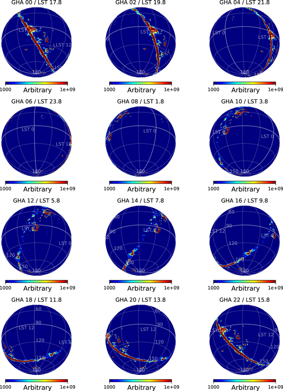
Figure 6. Simulated all-sky RRL proxy maps for the center of each LST bin. The images are orthographic projections of the Planck 2015 CO map at 115.27 GHz (Adam et al. 2016; Ade et al. 2016), which provides a rough proxy for the location of carbon in the Galaxy. The CO line emission is tightly concentrated along the Galactic plane, similar to RRL surveys of the plane.
Download figure:
Standard image High-resolution image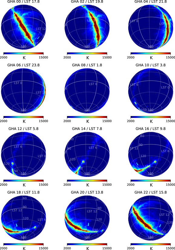
Figure 7. Same as Figure 6, but for the total radio emission visible by EDGES derived from the Haslam et al. (1981) 408 MHz sky map scaled to 70 MHz using a spectral index of β = − 2.4. The maps are dominated by synchrotron and free–free emission, which extends from the Galactic plane to higher latitudes compared to the CO emission observed by Planck.
Download figure:
Standard image High-resolution imageIn Figure 8, we show the simulated drift scans along with EDGES Cα and Hα observations, all normalized to their maximum amplitudes at LST 18 hr. The CO proxy map reasonably reproduces the relative LST trends of the Cα and Hα drift scans observed by EDGES, capturing the peak-to-peak range and the temporal width of the cycle more closely than the synchrotron continuum map. This is consistent with RRLs being more concentrated on the Galactic plane than synchrotron emission. Despite capturing the broad trends, the simplistic CO proxy fails to predict the relative RRL amplitudes and trends with LST observed between LST 0 and 10 hr, suggesting that it is a poor template for predicting RRLs in regions of the sky of most interest to redshifted 21 cm power spectrum observations.
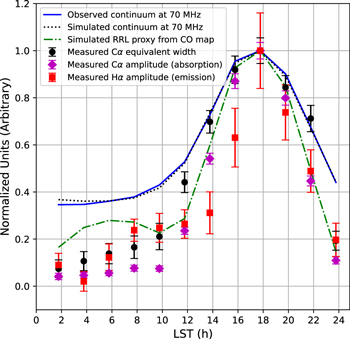
Figure 8. Peak normalized comparison of measured RRL strength and simulated proxy measurements as a function of LST. The average line profile magnitudes for Cα (purple diamonds) and Hα (red squares) are shown along with the Cα integrated optical depths (black circles). The simulated proxy measurement based on the Planck 115.27 GHz CO map (dashed–dotted green line) provides a reasonable predictor of relative RRL strength, particularly when the Galactic center is in the beam. However, it overpredicts the RRL strength at low LST. For reference, the continuum drift scan from EDGES observations (solid blue line) is plotted along with a simulated continuum drift scan using the Haslam et al. (1981) 408 MHz map (dotted black line). As expected, the continuum drift scans show a broader peak than the RRL scans, consistent with synchrotron emission extending farther from the Galactic plane compared to line emission.
Download figure:
Standard image High-resolution image3.5. Extending to 124.5 MHz
Here we repeat the line analysis for data from the EDGES mid-band instrument using 66 days of observations from early 2020. The mid-band instrument uses a smaller antenna than the low-band instrument, shifting the frequency range to 60–160 MHz. At 90 MHz, the mid-band antenna beam has FWHM of 754 parallel to excitation axis in the north–south direction and 106
6 perpendicular (Monsalve et al. 2021). For this analysis, we reduce the frequency range to 108–124.5 MHz, following a conservative approach of excluding RFI from FM band below 108 MHz and from satellite communication bands and air-traffic control channels above 125 MHz. Even in this narrow band, some of the frequency channels are dominated by RFI and thus need rigorous flagging. We completely discard time bins that have 60% or more of the frequency channels flagged. We fit and remove the continuum using an 11-term polynomial and further clean the data by discarding days with residual amplitudes larger than 10 K.
From Equation (1), we expect 18 RRL Cα transitions (375 ≤ n ≤ 392) in the frequency range of 108–124.5 MHz that are roughly spaced 1 MHz apart. We select 600 kHz windows around each line center and stack these segments from the continuum-removed residual spectra, resulting in an effective mean frequency of 116.3 MHz. We expect similar LST dependence to low-band results, and thus, for simplicity, we only investigate two LST bins: (1) a 2 hr bin centered on LST 18 hr, when the Galactic center is overhead, and (2) a large 12 hr bin centered on LST 6 hr, when the Galactic center is not overhead. The average line profile was fit in each bin with a double-Gaussian model for hydrogen emission and carbon absorption.
In the LST 18 hr bin, at a center frequency of 116.3 MHz, we find a best-fit amplitude of –46 ± 15 mK and FWHM of 73.4 ± 56 kHz for Cα and 98 ± 38 mK and FWHM of 48.9 ± 15 kHz for Hα, as shown in Figure 9. We can also correct for beam dilution and compare these observations to existing RRL surveys. The EDGES mid-band antenna is a scaled copy of the low-band antenna; hence, it has similar beam properties, and the dilution factors we calculated earlier are still valid. Accounting for the dilution effects and using an undiluted continuum temperature of 6980 K, we find an undiluted Hα amplitude of about 4 K with τ dv ≈ − 8 Hz and L/C ≈ 5 × 10⁻⁴. Cα has an undiluted amplitude of 2 K with τ d ν ≈ 6 Hz with L/C ≈ − 2 × 10⁻⁴. Away from the Galactic center in the large LST bin centered on 6 hr, we find the best-fit amplitude for Cα of 3.4 ± 3.5 mK, consistent with no detection, and yielding a 3σ upper limit of 14 mK. Similarly, we see no evidence of Hα emission present and can assign a comparable upper limit.
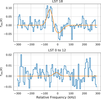
Figure 9. Stacked line profiles (blue) in mid-band EDGES data spanning the frequency range 108–124.5 MHz, with 375 ≤ n ≤ 392 and effective mean frequency of 116.3 MHz. The top panel shows a 2 hr LST bin centered on the Galactic center. A double-Gaussian model (orange) gives a best-fit Cα amplitude of −46 ± 15 mK. The best-fit Hα amplitude of 98 ± 38 mK, peaking 59 kHz below the carbon absorption, is about half of the peak level found at lower frequencies. The bottom panel shows a long 12 hr bin centered on LST 6 hr, yielding stacked line profiles consistent with no detection (best-fit Cα amplitude of 3.4 ± 3.5 mK).
Download figure:
Standard image High-resolution image3.6. Frequency Dependence of RRLs
In this section, we investigate the frequency dependence of Cα, Cβ, and Hα line amplitudes within the observed bands and compare the EDGES observations to prior observations and theoretical expectations. The observed temperature brightness of the lines relative to the background is dependent on the electron temperature (Te
; Shaver 1980), optical depth of the lines ( ), and background radiation temperature (TR
). The assumption of local thermodynamic equilibrium (LTE) may not hold for n ≳ 100 (Salgado et al. 2017b), resulting in increased contributions from stimulated emission or absorption. In this regime, observed line temperatures relative to the total continuum can be written as
), and background radiation temperature (TR
). The assumption of local thermodynamic equilibrium (LTE) may not hold for n ≳ 100 (Salgado et al. 2017b), resulting in increased contributions from stimulated emission or absorption. In this regime, observed line temperatures relative to the total continuum can be written as

where bn
and βn
are departure coefficients (Gordon & Sorochenko 2009) accounting for deviations from LTE and νn
is the frequency corresponding to a specific transition line. For the low-frequency, large-n lines observed here,  is effectively constant with frequency owing to the nearly identical Saha–Boltzmann occupations for nearby n and low photon energy relative to the excitation temperature. The departure coefficients are smooth functions of n, although they may have multiple inflection points. For Cα they can span 0.6 ≲ bn
≲ 1.3 and −20 ≲ bn
βn
≲ 15, depending on the density and temperature of the gas (Salgado et al. 2017b), which are expected to be ne
≈ 0.1 cm−3 and Te
≈ 50–100 K, respectively.
is effectively constant with frequency owing to the nearly identical Saha–Boltzmann occupations for nearby n and low photon energy relative to the excitation temperature. The departure coefficients are smooth functions of n, although they may have multiple inflection points. For Cα they can span 0.6 ≲ bn
≲ 1.3 and −20 ≲ bn
βn
≲ 15, depending on the density and temperature of the gas (Salgado et al. 2017b), which are expected to be ne
≈ 0.1 cm−3 and Te
≈ 50–100 K, respectively.
The sky continuum temperature is dominated by synchrotron and free–free emission at low radio frequencies and follows a power law,  K, where β is the spectral index and T100 is a normalizing temperature at ν100 = 100 MHz. The observed sky temperature from Earth toward the inner Galactic plane is about 10,000 K at 100 MHz, falling to about 1000 K away from the plane (Dowell et al. 2017). The gas that produces RRLs is at varying distances from Earth. Some of the synchrotron and free emission we observe originates between Earth and the gas. This portion of the received emission does not experience RRL absorption in the gas and is not included in the radiation background, TR
, in Equation (7). To account for this, TR
is typically approximated as a fraction of Tcont.
K, where β is the spectral index and T100 is a normalizing temperature at ν100 = 100 MHz. The observed sky temperature from Earth toward the inner Galactic plane is about 10,000 K at 100 MHz, falling to about 1000 K away from the plane (Dowell et al. 2017). The gas that produces RRLs is at varying distances from Earth. Some of the synchrotron and free emission we observe originates between Earth and the gas. This portion of the received emission does not experience RRL absorption in the gas and is not included in the radiation background, TR
, in Equation (7). To account for this, TR
is typically approximated as a fraction of Tcont.
In Figure 10, we show the frequency dependence of the Cα and Cβ lines measured by EDGES. To place the EDGES observations on the same scale as previously reported results from other instruments, we use undiluted  line amplitude estimates instead of the directly measured values. To estimate the undiluted
  of individual lines, we use the amplitude of the continuum-subtracted residual spectrum at each line center frequency. The 1σ uncertainty for each line is estimated from the residual spectrum rms, scaled to each line frequency by a power law matching the sky spectrum. For LST 18 hr, we plot the undiluted estimates and compare them with the Oonk et al. (2019) and Erickson et al. (1995) observations of the Galactic center region. The Oonk et al. (2019) data were reported as τ
d
ν integrals, where τ = TRRL/Tcont is the observed line-to-continuum ratio. To convert them to brightness temperature units, we estimate τ from their reported τ
d
ν and FWHMline and then multiply by Tcont assuming β = − 2.4 and T100 = 10,000 K, appropriate for the inner Galactic plane. We use the reported nondetections as τ
d
ν = 0 and the associated upper limits as error bars on τ
d
ν. We also calculate and correct for beam dilution factors for each of their measurements using their reported FWHMbeam values and treating them as the diameters of circular top hat areas in solid angle. The beam dilution factors increase from 0.63 at 40 MHz to unity (no dilution) at 87 MHz and above. Erickson et al. (1995) report the line amplitudes scaled by the system temperature. With an FWHMbeam of 4° at 76.4 MHz, the line amplitudes are likely not beam diluted, and we apply no correction. We take 35 of the total 43 reported fields from the line-forming region with Galactic longitudes l = 340° to l = 20°, ignoring eight regions with unreported system temperature and those with nondetections. We rescale them with the reported system temperature and calculate an effective mean line amplitude of –7.9 ± 0.9 K at an effective mean frequency of 76.4 MHz for C348α–C444α. Even with the simple assumptions and approximations used to place all of the observations on the same scale, we see good agreement between the line amplitudes measured here and those previously reported by Oonk et al. (2019) and Erickson et al. (1995). We repeat a similar process for the middle row of Figure 10 to show the undiluted
of individual lines, we use the amplitude of the continuum-subtracted residual spectrum at each line center frequency. The 1σ uncertainty for each line is estimated from the residual spectrum rms, scaled to each line frequency by a power law matching the sky spectrum. For LST 18 hr, we plot the undiluted estimates and compare them with the Oonk et al. (2019) and Erickson et al. (1995) observations of the Galactic center region. The Oonk et al. (2019) data were reported as τ
d
ν integrals, where τ = TRRL/Tcont is the observed line-to-continuum ratio. To convert them to brightness temperature units, we estimate τ from their reported τ
d
ν and FWHMline and then multiply by Tcont assuming β = − 2.4 and T100 = 10,000 K, appropriate for the inner Galactic plane. We use the reported nondetections as τ
d
ν = 0 and the associated upper limits as error bars on τ
d
ν. We also calculate and correct for beam dilution factors for each of their measurements using their reported FWHMbeam values and treating them as the diameters of circular top hat areas in solid angle. The beam dilution factors increase from 0.63 at 40 MHz to unity (no dilution) at 87 MHz and above. Erickson et al. (1995) report the line amplitudes scaled by the system temperature. With an FWHMbeam of 4° at 76.4 MHz, the line amplitudes are likely not beam diluted, and we apply no correction. We take 35 of the total 43 reported fields from the line-forming region with Galactic longitudes l = 340° to l = 20°, ignoring eight regions with unreported system temperature and those with nondetections. We rescale them with the reported system temperature and calculate an effective mean line amplitude of –7.9 ± 0.9 K at an effective mean frequency of 76.4 MHz for C348α–C444α. Even with the simple assumptions and approximations used to place all of the observations on the same scale, we see good agreement between the line amplitudes measured here and those previously reported by Oonk et al. (2019) and Erickson et al. (1995). We repeat a similar process for the middle row of Figure 10 to show the undiluted  of Cα and Cβ lines measured by EDGES away from the inner Galactic plane in a large LST 0–12 hr averaged bin. In this case, however, there are no comparable observations from other instruments for comparison.
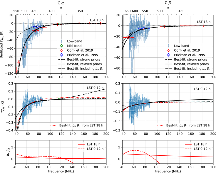
Figure 10. Frequency dependence of Cα and Cβ absorption lines. The top panels shows LST 18 hr after correcting for beam dilution and spectral smearing. The middle panels shows the average over LST 0–12 hr assuming that the lines are due to diffuse gas filling the beam; hence, no beam dilution correction is applied. In both cases, EDGES low-band data (blue circles) have a strong frequency dependence. A single mid-band point (green square) for Cα represents the average across its analyzed data. For LST 18 hr, the Oonk et al. (2019) data (red diamonds) and a composite of the Erickson et al. (1995) data (blue square) are shown after adjusting to brightness temperature units as described in Section 3.6. 1σ error bars are plotted for all points but do not include dilution uncertainty in the LST 18 hr case, which is conservatively estimated as a 50% error in undiluted  . Overall, there is good agreement between this work and Oonk et al. (2019). The black solid and dashed lines show best-fit models in the LTE limit of Equation (7) as described in Section 3.6. The black dashed–dotted lines show the best-fit model when the departure coefficient product, bn
βn
, is modeled as a third-order polynomial in frequency and included in the parameter estimation with the strong priors. The best-fit departure coefficient models are shown in the bottom panel. For LST 18 hr, the best-fit bn
βn
for Cα qualitatively resembles the curves in Salgado et al. (2017b).
. Overall, there is good agreement between this work and Oonk et al. (2019). The black solid and dashed lines show best-fit models in the LTE limit of Equation (7) as described in Section 3.6. The black dashed–dotted lines show the best-fit model when the departure coefficient product, bn
βn
, is modeled as a third-order polynomial in frequency and included in the parameter estimation with the strong priors. The best-fit departure coefficient models are shown in the bottom panel. For LST 18 hr, the best-fit bn
βn
for Cα qualitatively resembles the curves in Salgado et al. (2017b).
Download figure:
Standard image High-resolution imageAs a further check, we fit a model to the data using Equation (7) simplified to its LTE limit by setting bn = βn = 1. For LST 18 hr, we fit all three data sets jointly and initially assume Te = 100 K and TR (ν) = 0.2 × Tcont(ν), similar to the background radiation model used by Oonk et al. (2019). We again use T100 = 10,000 K and β = −2.4. We find a best-fit τL = 1.91 × 10⁻³ for Cα with a Bayesian information criterion (BIC) of 2938. This is shown as the “strong prior” model in Figure 10. Removing our assumptions for Te , T100, and β and including them in the parameter estimation improves agreement between data and model and is highly preferred, decreasing the BIC to 844. This “relaxed prior” fit yields Te = 190 K, T100 = 5550 K, β = −3.6, and τL = 5.01 × 10⁻³. Similarly, for Cβ, a strong prior fit yields τL = 1.62 × 10⁻³ with a BIC of 899, while a “relaxed prior” fit yields Te = 162 K, T100 = 9000 K, β = −2.7, and τL = 1.82 × 10⁻³ with a BIC of 854, thus favoring a relaxed prior model. While the relaxed priors yield good fits in both cases, the steep spectral index in the best-fit Cα model is unrealistic.
For the LST 0–12 hr case, which contains only EDGES observations, we test an analogous pair of strong and relaxed prior constraints. For the strong prior, we use T100 = 1000 K but retain Te = 100 K and β = −2.4. For Cα, we find τL = 1.29 × 10⁻⁴ with a BIC of 281. With relaxed priors we find best-fit Te = 10 K, T100 = 42, 965 K, β = −4.1, and τL = 1.10 × 10⁻⁶ with a BIC of 271, thus slightly favoring a relaxed prior model, but hitting the lower limit on the prior set to Te and finding an extreme T100. Similarly for Cβ, a strong prior model yields τL = 4.90 × 10⁻⁵ with a BIC of 366, while a relaxed prior model yields τL = 2.09 × 10⁻⁴, Te = 278 K, T100 = 1285 K, β = −1.0 with a BIC of 353, although here we hit the lower limit on the prior for β. The relatively low signal-to-noise ratio of the Cβ observations and more limited frequency range at LST 0–12 hr compared to LST 18 hr likely reduce the sensitivity to distinguish between the two models for the Cβ lines. Nevertheless, we again see unrealistic background radiation preferred in the relaxed prior cases.
For both LST 18 and 0–12 hr cases for Cα, the relaxed prior models prefer steep spectral indices for TR that are physically unrealistic. This suggests assuming that ideal LTE conditions may be insufficient to accurately capture the full frequency dependence of the line amplitudes along the inner Galactic plane between 40 and 200 MHz. A full treatment of bn and βn in the model could improve agreement with data without driving the models to extreme background radiation properties. It is beyond the scope of this work to incorporate detailed departure coefficient models, which are sensitive to Te and ne for each of the gas clouds in the observed fields, but we can test whether smoothly varying departure coefficients can provide useful degrees of freedom for the model to be consistent with the data without requiring extreme conditions for the gas or background radiation. Since bn has been calculated to remain close to unity and the background radiation brightness temperature is likely much larger than the gas temperature, we expect that RRL amplitudes in our observations are dominated by the TR term in Equation (7) and relatively insensitive to the Te term. We keep bn = 1 fixed and focus on the product bn βn = βn , for both Cα and Cβ cases. The departure coefficient models of Salgado et al. (2017b) show that βn is generally a monotonically varying smooth function for 300 ≲ n ≲ 550 for Cα and 490 ≲ n ≲ 700 for Cβ, over a large range of Te and ne . We account for this structure by modeling βn as a third-order (cubic) polynomial in frequency as

with M = 3. We fit for the βn
terms and  while otherwise following the strong prior scenario described above with fixed Te
, T100, and β. For Cα in the LST 18 hr case, including the polynomial for βn
yields good fits and is the most preferred model, lowering the BIC by 64 beyond the relaxed prior case, whereas for Cβ at LST 18 hr, including βn
is slightly less preferred, increasing the BIC by 5 over the relaxed prior case. For LST 0–12 hr, including the βn
polynomial is not preferred for both Cα and Cβ, with similar BIC to the relaxed prior model. Further, for the Cβ model fit, βn1 and βn3 hit their prior limits.
while otherwise following the strong prior scenario described above with fixed Te
, T100, and β. For Cα in the LST 18 hr case, including the polynomial for βn
yields good fits and is the most preferred model, lowering the BIC by 64 beyond the relaxed prior case, whereas for Cβ at LST 18 hr, including βn
is slightly less preferred, increasing the BIC by 5 over the relaxed prior case. For LST 0–12 hr, including the βn
polynomial is not preferred for both Cα and Cβ, with similar BIC to the relaxed prior model. Further, for the Cβ model fit, βn1 and βn3 hit their prior limits.
The bottom panel of Figure 10 shows the derived bn
βn
dependence on frequency. For LST 18 hr, it matches qualitatively with Salgado et al. (2017b, their Figure 8) and has a smoothly varying trend across the frequency range with 0.79 < bn
βn
< 4.5. With its higher values at lower frequencies, this non-LTE extension absorbs the need for a steep spectral index in the background radiation found in the LTE limit. The LST 0–12 hr observations are more limited without accompanying measurements at high frequencies, and the best fit is not constrained by data above 120 MHz. This makes bn
βn
highly covariant with  . We had to fix
  to prevent the estimation from trending to unrealistically large
  and small bn
βn
. With this additional constraint, we found 0 < bn
βn
< 2.3 over the range of the data. If the gas in both LST cases has similar properties, we might expect that the better-constrained bn
βn
model from the LST 18 hr data would also improve the LST 0–12 hr fits. Using that polynomial instead of bn
= βn
= 1 and fixing all other parameters except
and small bn
βn
. With this additional constraint, we found 0 < bn
βn
< 2.3 over the range of the data. If the gas in both LST cases has similar properties, we might expect that the better-constrained bn
βn
model from the LST 18 hr data would also improve the LST 0–12 hr fits. Using that polynomial instead of bn
= βn
= 1 and fixing all other parameters except  with the strong prior assumptions decreases the BIC by nearly 3, making it the most preferred model for the LST 0–12 hr case.
We repeat a similar analysis to show the frequency dependence of Hα for the LST 18 hr case. We apply the beam dilution and spectral smearing factors for EDGES low band and EDGES mid-band as described in Section 3.2 and use the Hα observations and instrument properties reported in Oonk et al. (2019) to place their data on the same temperature scale. Similar to Cα and Cβ, we see a good agreement between the measurements reported here and those in Oonk et al. (2019), providing further evidence that our simple approximations for placing all observations on the same scale are reasonable. We again use Equation (7) and begin by fitting in the LTE limit with relaxed priors. This yields  , Te
= 9925 K, T100 = 5000 K, β = −3.84 with a BIC of 571 and is shown as the best-fit relaxed prior case in Figure 11. The model is in poor agreement with the data, failing to capture the increase in amplitude with decreasing frequency and again resulting in an unrealistically steep best-fit spectral index for the background radiation.
, Te
= 9925 K, T100 = 5000 K, β = −3.84 with a BIC of 571 and is shown as the best-fit relaxed prior case in Figure 11. The model is in poor agreement with the data, failing to capture the increase in amplitude with decreasing frequency and again resulting in an unrealistically steep best-fit spectral index for the background radiation.
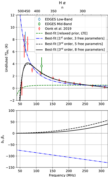
Figure 11. Frequency dependence of Hα emission lines for the LST 18 hr case. We show the undiluted line amplitude of EDGES low band and EDGES mid-band, along with the results from Oonk et al. (2019) after adjusting to brightness temperature units following the same process as for Cα and Cβ in Figure 10. Again, we see reasonable agreement between the EDGES and Oonk et al. (2019) observations. The green dashed line shows the best-fit model in the LTE limit. The blue dashed line shows the best-fit model for a non-LTE case using the strong priors described in Section 3.6 and with bn = 1 and bn βn modeled as a first-order (linear) polynomial. The black solid and dashed lines show the best-fit models in the non-LTE limit of Equation (7), where βn is further expanded as a third-order polynomial. The bottom panel shows the derived models of bn βn in the non-LTE cases.
Download figure:
Standard image High-resolution imageAs with the carbon lines, the poor agreement motivates exploring the models for Hα in non-LTE conditions. To do so, we assume a hot hydrogen gas scenario and use the strong priors to fix Te
= 7000 K, T100 = 10, 000 K, β = −2.4, and bn
= 1. We fit only for  and the βn
components of a first-order (linear) polynomial using M = 1 in Equation (8). This yields a best fit with a negative bn
βn
component,
and the βn
components of a first-order (linear) polynomial using M = 1 in Equation (8). This yields a best fit with a negative bn
βn
component,  , and a BIC of 171. The model is now in reasonable agreement with the data, although the lowest-frequency measurement of Oonk et al. (2019) at 55.7 MHz suggests that an unmodeled turnover may occur.
Extending the βn
model to the full third-order polynomial (M = 3) allows it to capture the apparent turnover at the lowest frequencies. We show the result of using the third-order polynomial and the same strong prior constraints as above in Figure 11 as the case with five free parameters. It yields a positive bn
βn
contribution with  and a BIC of 26. Relaxing all priors (labeled as eight free parameters in Figure 11), we find a best-fit bn
βn
contribution similar to the strong prior case along with
and a BIC of 26. Relaxing all priors (labeled as eight free parameters in Figure 11), we find a best-fit bn
βn
contribution similar to the strong prior case along with  , Te
= 3954 K, T100 = 15,400 K, β = −2.98, and a BIC of 32. Thus, the non-LTE strong prior case with five free parameters is favored among all models. Given the sensitivity of bn
βn
to the lowest-frequency data point reported by Oonk et al. (2019), more observations around and below 50 MHz would be valuable.
, Te
= 3954 K, T100 = 15,400 K, β = −2.98, and a BIC of 32. Thus, the non-LTE strong prior case with five free parameters is favored among all models. Given the sensitivity of bn
βn
to the lowest-frequency data point reported by Oonk et al. (2019), more observations around and below 50 MHz would be valuable.
Table 3 lists the best-fit model parameters for Cα, Cβ, and Hα lines in the LTE limit with relaxed priors and in the non-LTE scenario with strong priors and a third-order polynomial for βn . Note that we only report the best-fit model parameters without their associated statistical uncertainties because errors are likely driven more by biases in our simple assumptions for scaling measurements onto the same temperature scale than by the statistical uncertainties in the fits.
Table 3. Best-fit Models of RRLs
| Line | LST | LTE | Non-LTE | ||||||||||
|---|---|---|---|---|---|---|---|---|---|---|---|---|---|

| Te | T100 | β |

| Te | T100 | β |

|

|

|

| ||
| (K) | (K) | (K) | (K) | ||||||||||
| Cα | 18 hr | 5.01 × 10⁻³ | 190 | 5550 | −3.6 | 8.71 × 10⁻³ | 100 | 10,000 | −2.4 | 0.30 | −0.60 | 0.56 | 0.03 |
| 0–12 hr | 1.10 × 10⁻⁶ | 10 | 42,965 | −4.1 | 1.26 × 10⁻⁴ | 100 | 1000 | −2.4 | 1.05 | −0.33 | −7.82 | −17.89 | |
| Cβ | 18 hr | 1.82 × 10⁻³ | 162 | 9000 | −2.7 | 9.75 × 10⁻⁴ | 100 | 10,000 | −2.4 | 1.53 | −0.94 | 0.25 | 0.008 |
| 0–12 hr | 2.09 × 10⁻⁴ | 278 | 1285 | −1.0 | 1.26 × 10⁻⁵ | 100 | 1000 | −2.4 | 0.71 | −20.00 | −14.61 | 20.00 | |
| Hα | 18 hr | 5.01 × 10⁻⁵ | 9925 | 5000 | −3.84 | 8.91 × 10⁻³ | 7000 | 10,000 | −2.4 | 0.65 | −2.29 | 4.37 | 0.59 |
Note. Best-fit parameters for LTE and non-LTE models of the frequency dependence of Cα, Cβ, and Hα lines using Equation (7). For the LTE model, bn = βn = 1. For the non-LTE model, Te , T100, and β are fixed matching the strong prior cases described in Section 3.6, bn = 1, and βn is represented by a third-order polynomial in frequency following Equation (8). The data and models are plotted in Figures 10 and 11.
Download table as: ASCIITypeset image
The LTE models presented in Shaver (1975b) and Salgado et al. (2017a) show increasing amplitudes of Hα lines with increasing frequency that are inconsistent with the amplitude changes observed by EDGES from 66 to 116 MHz and with our interpretation of the data reported in Oonk et al. (2019). However, including the departure coefficients in the models improves agreement with the data, suggesting that the more sophisticated non-LTE treatment is necessary to model the spectral dependence of RRLs at the observed frequencies. Thus, collectively, these findings are consistent with theoretical analyses that show that non-LTE effects are significant at large n for lower-density, higher-temperature gas, such as Shaver (1975b, their Figure 5). Both negative and positive best-fit ranges of bn βn are allowed in the models of Salgado et al. (2017a), depending on the electron temperature and density of the gas.
We briefly consider alternative explanations for the decrease in Hα amplitude with frequency other than non-LTE physics. Strong Hα emission lines may be preferentially flagged during the RFI excision in our analysis, particularly in the mid-band data; however, we find no bias in the flag counts at the frequencies corresponding to Hα lines. Overlap between the Hα and Cα lines could hinder the model fitting; however, our synthetic tests on the two-component model with varying separation of Cα and Hα lines (20–100 kHz) show confident retrieval of line parameters with less than 5% error for all line parameters that have at least 20 kHz separation, while the model fails to retrieve the hydrogen line parameters at 10 kHz separation, and the errors on carbon line parameters rise to 15%. This establishes robustness against such confusion unless there was an unknown systematic offset between the radial velocities of hydrogen and carbon clouds that causes them to overlap more than expected.
Oonk et al. (2019) report evidence for a nearby cold hydrogen cloud along the line of sight to the Galactic center based on a narrowing of the Hα line width with decreasing frequency from 25 km s−1 between 300 and 80 MHz to 12 km s−1 in their lowest-frequency detections at 73 and 63 MHz. This could be explained by beam dilution effects: as the beam size increases at lower frequencies, it could encompass more of an extended nearby cloud of cooler gas than the Galactic center region compared to beam at higher frequencies. Such effects are less likely for the EDGES observations, which have nearly constant beam size; hence, the relative dilution of different regions should not change with frequency. The other possible explanations could be due to line blending with Cα lines; however, we see a similar scaling in line width to that of Oonk et al. (2019; a factor of 2.5 from 12 ± 3.7 km s−1 at 63 MHz and 29 ± 3.7 km s−1 at 113 MHz for Oonk et al. 2019, and a factor of 2.8 from 77 ± 9 km s−1 at 66.7 MHz and 221.6 ± 68 km s−1 at 116 MHz for EDGES). Further, we find the Oonk et al. (2019) observations to be consistent with the  derived from EDGES, suggesting little change in line blending due to frequency-dependent beam dilution since the two instruments have different beam characteristics—although the uncertainties are large in both cases, suggesting the need for more precise measurements.
4. Implications for 21 cm Observations
Summarizing the findings from Section 3.3 for diffuse RRL contributions away from the Galactic center, we have detected C α absorption at about 30–40 mK and placed upper limits on Cβ absorption and Hα emission lines at 30 mK levels in the 50–87 MHz band. In the 108–124 MHz band, we have placed upper limits on Cα absorption and Hα emission at about 14 mK. These levels are generally at or below the expected redshifted 21 cm angular and spectral fluctuation amplitudes in theoretical models (e.g., Furlanetto et al. 2004; Barkana 2009; Fialkov & Barkana 2019), which are typically 10–100 mK, depending on model and redshift. Here we empirically study the quantitative effects induced by RRLs on the global and power spectrum of 21 cm signal using the amplitudes of the detected lines.
4.1. Global 21 cm Signal
Early results in the search for the global 21 cm signal (e.g., Monsalve et al. 2017a; Bowman et al. 2018; Singh et al. 2018, 2022) have generally ignored the presence of RRLs. To test whether this is a reasonable assumption, we create simulated observations to investigate the recovery of the global 21 cm signal with and without the strongest RRLs in an extreme scenario assuming that the measurement is made at LST 18 hr, when the strong lines on the inner Galactic plane are present.
To model the carbon absorption lines, we include all individual Cα lines in the full EDGES low band of 50–100 MHz by scaling the measured stacked line amplitude in frequency and adding Gaussian profiles with 19.8 kHz FWHM at each line center. For the frequency scaling, we note that for the target frequencies Equation (7) is dominating by the TR term. We therefore simplify the expression and use only a power law:

where A is the best-fit stacked amplitude at LST 18 hr from Table 1, νeff = 66.1 MHz is the effective frequency of our observations, and β is the best-fit spectral index for the relaxed prior LTE model in Table 3. For Cα lines we use A = −0.795 K and β = −3.6, while for Cβ we use A = −0.261 K and β = −2.7.
Hα emission lines are added with a constant amplitude of 203 mK, as an extreme case of the highest detected amplitude representing all the lines in the full frequency band. This RRL model has an rms of 207 mK for a simulated spectrum with 6 kHz resolution, matching the raw resolution of the EDGES data. The rms reduces to 101 mK after binning to 61 kHz, which matches the spectral resolution of SARAS (Singh et al. 2022), and 14 mK after binning to the 390 kHz resolution used in Bowman et al. (2018). The noise falls faster than the square root of the channel size because, for large spectral bins, some of the emission and absorption lines fall in the same bins, offsetting their contributions to the rms. At the respective spectral resolutions, the rms is below the thermal noise, which is about 25 mK for deep EDGES observations and about 200 mK for SARAS (Singh et al. 2022). Hence, we expect that the RRLs will have little impact on the signal recovery.
To test signal recovery, we start by extracting a realistic foreground continuum model from the EDGES observations used in Bowman et al. (2018). We use edges-analysis 8 to calibrate the data and flag RFI, correct for beam chromaticity, and bin the observations between LST 17 and 18 hr. We simultaneously fit a five-term linearized logarithmic polynomial (“linlog”) foreground model and a five-term flattened Gaussian 21 cm absorption profile. We use this best-fit foreground model as the continuum in the simulated observations. We then add the RRL model and a modeled 21 cm absorption feature matching the best-fit properties reported in Bowman et al. (2018), but with a conservative amplitude of 200 mK. When we fit a five-term linlog foreground model and 21 cm absorption flattened Gaussian profile simultaneously to the simulated observations, the difference in amplitude of the best-fit global 21 cm absorption feature with and without the RRLs is about 2 mK, extremely small compared to the 200 mK injected signal. Figure 12 shows the RRL model and resulting global 21 cm fit. Lastly, we tested flagging RRLs in the analysis of actual observations and found that it did not affect the results reported in Bowman et al. (2018).
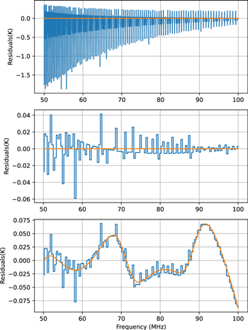
Figure 12. Top: residuals after fitting and removing a five-term foreground model from simulated spectra in the 50–100 MHz band at LST 18 hr with 6 kHz resolution. The orange curve shows the residuals to a model without RRLs, whereas the blue curve includes modeled Cα, Cβ, and Hα lines. Middle: the residuals rebinned to 390 kHz for comparison with Bowman et al. (2018). Bottom: residuals after the foreground model is fitted and removed when a 200 mK flattened Gaussian global 21 cm absorption signal is also included in the simulated spectra. RRLs contribute to an increase in rms by 12 mK in the data. The difference in amplitude of the best-fit 21 cm profile is only 2 mK, an error of 1%.
Download figure:
Standard image High-resolution imageThese findings apply directly to EDGES observations. They also should be representative of most other global 21 cm experiments since most instruments have large beams that would similarly dilute the observed amplitude of strong lines from the inner Galactic plane. We note, however, that the effects of RRLs on global 21 cm searches could be more significant for instruments with higher angular resolution.
4.2. 21 cm Power Spectrum
Interferometers optimized for 21 cm power spectrum observations aim to detect and characterize the IGM during cosmic dawn and reionization. Most instruments have focused on observing the reionization era between 13 > z > 6, corresponding to frequencies between 100 and 200 MHz. Recently, several instruments have begun to place initial upper limits on the 21 cm signal during cosmic dawn between 25 > z > 15, between about 50 and 90 MHz (Eastwood et al. 2019; Gehlot et al. 2019, 2020). During reionization, fluctuations in the 21 cm signal are dominated by the growth of reionized regions on scales of order 10 Mpc, corresponding to spectral fluctuations on scales of order 1 MHz in observations, although there is also a significant power on smaller scales. Before reionization, the 21 cm power spectrum traces the matter power spectrum and ultraviolet and X-ray heating of the IGM, yielding power on generally similar scales to those during reionization. The amplitude of 21 cm fluctuations is predicted to be Δ2 ≲ 102 mK2, varying with redshift as the IGM evolves. Although there have been significant improvements in upper limits of 21 cm power spectrum measurements in the past decade, the current best upper limits are an order of magnitude higher than the fiducial model (Barry et al. 2021; Abdurashidova et al. 2022).
Here we estimate the approximate power contributed by RRLs over these spectral scales in a typical observation by simulating all Cα, Cβ, and Hα RRLs spanning 50–100 MHz following a similar method to that for the global 21 cm test but using the average line amplitudes and limits found for LSTs 0–12 hr. These lines are much weaker than those along the inner Galactic plane. This analysis is directly relevant for the 21 cm interferometers targeting cosmic dawn between 25 > z > 15, including OVRO-LWA, LOFAR, and AARTFAAC. The Hydrogen Epoch of Reionization Array (HERA; DeBoer et al. 2017; Abdurashidova et al. 2022) is also sensitive down to 50 MHz, although it is optimized for 100–200 MHz to observe reionization. We focus our analysis here on HERA given our familiarity with the instrument.
To simulate observations including RRLs, we use the best-fit strong prior model shown in the middle panel of Figure 10 as our reference for Cα amplitudes and a constant Hα amplitude of 33 mK across the band, which is the average from the individual 2 hr LST bins centered between 0 and 12 hr. This model somewhat overestimates the line strength compared to the very weakest region of sky at LSTs 2–6 hr but will be more typical of the region covered by long drift scans with HERA. We note that instruments like HERA have high angular resolution (08 at 75 MHz) in comparison to EDGES (72° at 75 MHz). Here we study a monopole-like RRL contribution that is assumed to be uniform over the full beam of HERA, focusing on the spectral line-of-sight effects rather than the angular effects. The resulting simulated spectra have 14 mK rms when the lines are fully resolved at 1 kHz resolution, falling to 6 mK rms when binned with 100 kHz resolution, typical of HERA observations. We note that, due to the smaller beam of HERA, one could expect lower line blending as compared to EDGES.
Figure 13 shows the simulated RRL contribution to HERA spectra and the corresponding delay spectra for different spectral resolutions. The delay spectra are found by applying a Blackman–Harris window function to the simulated sky spectra and Fourier transforming into delay space. The delay spectra are equivalent to what would be seen by a zero-length baseline in an interferometer if the sky contained only RRLs. They illustrate that much of the power introduced by the RRLs resides on small spectral scales below 500 kHz, corresponding to delays greater than 2 μs. The limited spectral resolution of HERA couples some of this small-scale power to larger scales, but the total power contributed by scales larger than 500 kHz accounts for less than 10 mK2 of the total 36 mK2 variance in the 100 kHz binned spectrum. These variances are two orders of magnitude lower than the current best upper limits at high redshift of Δ2 ≤ 3496 mK2 at z = 10.4 (HERA Collaboration et al. 2023) and Δ2 ≤ 7388 mK2 at z = 17.9 − 18.6 (Gehlot et al. 2020). The RRL power will likely be lower on nonzero-length baselines, falling quickly with baseline length similar to other diffuse Galactic emission. Future work to map the spatial distribution of RRLs would be valuable to confirm this assumption. The levels of systematics introduced owing to RRLs may need to be considered in next-generation instruments. Nevertheless, the power levels introduced by RRLs are at the low end of expected 21 cm signal levels, and we anticipate that the lines can likely be ignored in the current generation of 21 cm interferometers, which are focused on detection and not detailed characterization of the signal.
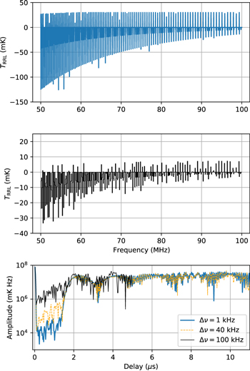
Figure 13. Top: simulated RRL spectrum, similar to Figure 12 but for LST 0–12 hr, away from the inner Galactic plane. Cα, Cβ, and Hα lines are modeled in the 50–100 MHz band with 1 kHz resolution. No other foreground contributions are included. Middle: the simulated spectrum rebinned to 100 kHz, which is approximately the spectral resolution used by HERA. Bottom: delay spectra calculated from the simulated RRLs for three different spectral binnings. These are equivalent to delay spectra from a notional zero-length baseline in an interferometer. Most of the power contributed by the RRLs is above 2 μs delay, corresponding to spectral scales smaller than 500 kHz. The 100 kHz spectral resolution of HERA couples power from smaller scales to larger scales of order 1 MHz. An intermediate spectral resolution of 40 kHz removes much of the coupling to large scales. Even with coupling, the power from scales larger than 500 kHz (<2 μs) contributes less than 10 mk2 to the total 36 mk2 variance in the simulated spectrum with HERA-like resolution.
Download figure:
Standard image High-resolution imageIn the ultimate case that the lines cannot be neglected initially, two scenarios are possible. First, if our assumption that diffuse weak lines dominate the observations is incorrect and instead strong lines from several small regions do indeed dominate, then the diffuse contribution would be even lower than our estimated upper limits above. Surveys of the localized dominant regions would likely enable them to be subtracted from 21 cm observations during processing with reasonable accuracy. Second, if diffuse lines are present across large areas of the sky at levels that interfere with the 21 cm analysis as may be possible (see, e.g., Grenier et al. 2005), then those frequencies may need to be completely omitted from analysis.
To investigate possible spectral leakage effects that RRL flagging could have on 21 cm power spectrum analysis, we use pyuvsim to simulate observations with HERA. HERA is a 350-element radio interferometer being built in South Africa for observing redshifted 21 cm power spectrum. HERA is designed to observe in the frequency range of 50–250 MHz. We simulate HERA visibilities at LST 0, 6, 12, and 18 hr on 18 baselines for the telescope's east–west polarization using the Global Sky Model (de Oliveira-Costa et al. 2008). The resulting visibilities are then passed through a Blackman–Harris window and transformed into delay space both before and after masking RRL channels. We apply a delay-inpainting algorithm in the masked delay spectra (Parsons & Backer 2009; Aguirre et al. 2022) and attempt to reconstruct the ideal observation as if RRLs had not been present. The inpainting algorithm is a deconvolution that effectively extrapolates along frequency for each visibility to fill in gaps due to RFI excision or other missing data. An example of the resulting delay spectra is shown in Figure 14 for LST 6 hr, which is broadly representative of all baselines and LSTs simulated. The effect of masking the RRL frequencies, even with inpainting, is to raise the noise floor in the modes of interest to 21 cm power spectrum analysis with absolute delays greater than about 0.1 μs by about two orders of magnitude. This limits the dynamic range to approximately 103, below the target performance of the telescope that is likely needed to detect the 21 cm power spectrum. This suggests that further development would be needed to identify successful strategies for mitigating diffuse RRLs in power spectrum analysis if flagging is required.
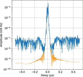
Figure 14. Comparison of simulated delay spectra for a baseline on the HERA radio telescope at LST 6 hr with and without assuming that RRL frequencies need to be masked. The dotted line shows the reference delay spectrum without flagging RRLs. Masking and inpainting RRL frequencies before the delay transform (solid line) raises the foreground leakage by over two orders of magnitude in the delay modes used for redshifted 21 cm science. A similar trend was observed for the other simulated LSTs and baselines in HERA.
Download figure:
Standard image High-resolution image5. Conclusions
We have used existing long drift scans from the EDGES low-band and mid-band instruments, with an effective spectral resolution of 12.2 kHz, divided into LST bins, to assess the strength of RRLs averaged over large areas of the sky. In the lower frequency range of 50–87 MHz, Cα absorption lines were seen at all LST periods, with amplitudes from −33 to −795 mK, and Hα lines were seen in emission, with average fitted amplitudes as a function of LST ranging from no detection to 203 mK. Cβ and Cγ lines were also seen in absorption with average fitted amplitudes between no detection and −305 mK and between no detection and −171 mK, respectively. At the higher frequency band of 108–124.5 MHz, RRL lines were seen only when the Galactic center was overhead. Hα lines were seen in emission with amplitude of 98 mK and Cα in absorption with an amplitude of −46 mK. We note that, due to large beam and line broadening, some line blending of absorption and emission lines may not be fully captured in our models.
Conservatively interpreting the observations away from the Galactic center as RRLs from diffuse gas, as opposed to isolated sources, we find that the amplitudes of the diffuse lines are at or below the expected redshifted 21 cm signal from cosmic dawn. They will likely have no impact on global 21 cm detection (assuming that the global 21 cm signal matches the current fiducial theoretical expectations of 50–100 mK) and are two orders of magnitude below current 21 cm power spectrum limits at high redshift. This suggests that Galactic RRLs do not impose significant systematics in low-frequency regimes and do not need mitigations in current 21 cm experiments. However, the power levels introduced by RRLs may need mitigation in the next generation of instruments aiming to characterize the 21 cm signal in detail after initial detections. A delay spectrum analysis for simulated HERA observations showed that if masking and inpainting RRL frequencies is required, foreground leakage could increase by about two orders of magnitude in the higher delay modes used for 21 cm analysis. This reduces the dynamic range in delay spectra to about 103, suggesting that new development would be needed in such a scenario. Further work is also warranted to extend this analysis to higher frequencies between 100 and 200 MHz, corresponding to the 21 cm redshifts for reionization, although the nondetection of Cα and Hα we find away from the inner Galactic plane at 116 MHz suggests that RRLs will be less of a problem for reionization observations than for higher-redshift cosmic dawn observations.
Acknowledgments
This work was supported by the NSF through research awards for EDGES (AST-1609450, AST-1813850, and AST-1908933) and by the NASA Solar System Exploration Research Virtual Institute cooperative agreement No. 80ARC017M0006. The authors thank the anonymous reviewer for detailed inputs and suggestions. The authors also thank Dr. Anish Roshi for useful discussions and providing relevant references. EDGES is located at the Inyarrimanha Ilgari Bundara, the CSIRO Murchison Radio-astronomy Observatory. We acknowledge the Wajarri Yamatji people as the traditional owners of the Observatory site. We thank CSIRO for providing site infrastructure and support.
Software: astropy (Astropy Collaboration et al. 2013, 2018), edges-analysis (http://github.com/edges-collab), pyuvsim (Lanman et al. 2019), pyuvdata (Hazelton et al. 2017).