Abstract
The mass accretion rates of young stellar objects (YSOs) are key to understanding how stars form, how their circumstellar disks evolve, and even how planets form. We develop a Bayesian framework to determine the accretion rates of a sample of 15 YSOs using archival data from the VIRUS spectrograph (R ∼ 800, 3500–5500 Å) on the Hobby–Eberly Telescope. We are publicly releasing our developed tool, dubbed nuts-for-ysos, as a Python package, which can also be applied to other spectroscopic data sets (https://github.com/laurenwillett/nuts-for-ysos). The nuts-for-ysos code fits a simple accretion model to the near-UV and optical continuum of each VIRUS spectrum. Our Bayesian approach aims to identify correlations between model parameters using the No U-Turn Sampler (NUTS). Moreover, this approach self-consistently incorporates all parameter uncertainties, allowing for a thorough estimation of the probability distribution for accretion rate not accomplished in previous works. Using nuts-for-ysos, we derive accretion rates of each YSO. We then verify the reliability of our method by comparing to results separately derived from only the spectral emission lines, and to results from earlier studies of the Lupus, Chamaeleon I, and NGC 1333 regions. Finally, we discuss what qualitative trends, covariances, and degeneracies were found among model parameters. The technique developed in this paper is a useful improvement that can be applied in the future to larger samples of YSOs observed by VIRUS or other spectrographs.
Original content from this work may be used under the terms of the Creative Commons Attribution 4.0 licence. Any further distribution of this work must maintain attribution to the author(s) and the title of the work, journal citation and DOI.
1. Introduction
Understanding how quickly a young star accretes mass is important for constraining models of circumstellar disk evolution and planet formation. Over the first few million years of their life, low-mass stars (≲2M⊙) possess a circumstellar disk that is dissipated mainly through photoevaporation, stellar winds, and accretion onto the star (R. Alexander et al. 2014). One commonly accepted paradigm is that young stellar objects (YSOs) in the class II phase accrete matter via magnetospheric accretion (Y. Uchida & K. Shibata 1985; A. Koenigl 1991; F. Shu et al. 1994; L. Hartmann et al. 2016). In this model, the stellar magnetic field couples to material from the inner circumstellar disk, and then guides gas along magnetic field lines onto the stellar surface. The gravitational energy released from this free-falling gas consequently heats up the gas and causes broad emission lines. The infalling material produces a “shock” when it encounters the stellar surface, heating up patches of the surface to about 104 K and creating UV continuum emission (E. Gullbring et al. 2000). Class III YSOs can still exhibit line emission like the younger accreting class II stars, but often to a lesser degree, and the emission is attributed mainly to the chromosphere rather than to accretion processes (C. F. Manara et al. 2013b).
Accretion directly “uses up” some of the circumstellar disk material. Moreover, the energy released from the accretion drives dissipation of material through outflows and photoevaporation of the disk. Finally, accretion influences the temperature and chemical composition of the inner disk. Through these channels, accretion therefore augments what material in the protoplanetary disk is available for planet formation. Deriving the mass accretion rate (Macc) of YSOs is therefore key to understanding both low-mass star formation and consequentially how planets may form around the star (C. F. Manara et al. 2019). In particular, the Macc–M⋆ empirical relation from class II YSOs has been heavily studied in order to probe changes in mass accretion over time (e.g., C. J. Clarke & J. E. Pringle 2006) and the related evolution in disks (e.g., B. Ercolano et al. 2014; C. F. Manara 2018, and references within).
Lacc is the total accretion luminosity: the luminosity from the YSO that can be attributed purely to the accretion process. Lacc can be treated as the release of gravitational potential energy during accretion, and therefore be converted into a mass accretion rate, Macc (see Equation (6) in Section 5.4). Accreting YSO spectra present continuum emission in excess of a main-sequence stellar photosphere, most notably through a “jump” in emission in the Balmer continuum (a “Balmer jump”) for wavelengths shortward of ∼3600 Å. The strength of this excess continuum emission can be used to estimate Lacc. Although not the only valuable wavelength range (for example, see the study of near-IR lines in E. Fiorellino et al. 2021; E. Fiorellino et al. 2023), the optical and near-UV wavelength range of a YSO spectrum therefore contains particularly useful information for estimating the total accretion luminosity Lacc. The typically high extinction of the YSO can make this a challenging regime for targeted observations, however, compared to the near-IR.
The “direct” method for determining Lacc involves fitting a model of the excess continuum emission to the YSO spectrum over a wide wavelength range. This direct method has been applied to numerous YSOs (e.g., J. A. Valenti et al. 1993; E. Gullbring et al. 1998; G. J. Herczeg & L. A. Hillenbrand 2008; E. Rigliaco et al. 2012; C. F. Manara et al. 2016; J. M. Alcalá et al. 2014, 2017). However, the techniques from previous literature have not been able to thoroughly examine degeneracy among model parameters. For example, the procedure described in C. F. Manara et al. (2013a) uses a discrete grid of parameter values and then finds the best fit by minimizing a likelihood function similar to a χ2 distribution (see Equation (4)). While this approach self-consistently determines Lacc, stellar spectral type, and extinction AV, it does not allow one to examine in detail the covariance of the parameters. Moreover, the uncertainty in Lacc has generally only been roughly estimated. For example in J. M. Alcalá et al. (2017), they state that the approximate uncertainty in Lacc is about ∼0.25 dex for log(Lacc/L⊙), and they qualitatively describe the contributors to this uncertainty. However, they do not include a precise quantitative accounting of the uncertainty in Lacc for each individual YSO. We aim to address these deficiencies using the same model as in C. F. Manara et al. (2013a), but in a Bayesian framework, to our collection of YSO spectra in Section 4. While we study a relatively small sample of YSOs, our work acts as a proof of concept for how the analysis of YSO spectra can be improved, and a demonstration of the new nuts-for-ysos tool.
The accretion luminosity Lacc can also be indirectly estimated by measuring the luminosities of a variety of emission lines (Lline) and then applying known empirical relationships between Lline and Lacc. For example, the strength of the He i lines, Ca ii lines, and both the visible and near-infrared hydrogen recombination lines has been shown to exhibit a correlation with the accretion luminosities of YSOs derived from the direct method (e.g., J. Muzerolle et al. 1998; G. J. Herczeg & L. A. Hillenbrand 2008; E. Rigliaco et al. 2012). Therefore, determining accretion luminosities from such emission lines is a reliable alternative, having yielded results that are consistent with the direct method, albeit with a higher scatter (G. J. Herczeg & L. A. Hillenbrand 2008; E. Rigliaco et al. 2012; J. M. Alcalá et al. 2014). Additional proxies besides emission-line fluxes include excess U-band emission (E. Gullbring et al. 1998), and the H-alpha 10% line width (A. Natta et al. 2004). These various “indirect” methods are useful for YSOs in which directly fitting a model of excess continuum emission near the Balmer jump is too difficult because the spectrum is low-signal-to-noise (due to high extinction in star-forming regions, or low throughput in transmission optics of the spectrograph, for example) or because the spectrum is only available over a narrow wavelength range.
Using either the direct method or indirect method, accretion rates have been acquired for YSOs in various star-forming regions including Taurus (E. Gullbring et al. 1998; J. Muzerolle et al. 2005), TWA (L. Venuti et al. 2019), ρ Oph (A. Natta et al. 2006), Chamaeleon I (J. Muzerolle et al. 2005; C. F. Manara et al. 2016, 2017b), η-Chamaeleon (M. Rugel et al. 2018), Lupus (J. M. Alcalá et al. 2014, 2017), Upper Scorpius (C. F. Manara et al. 2020), and NGC 1333 (E. Fiorellino et al. 2021), among others. M* and Macc for these stars have been shown to exhibit a loosely positive correlation, of roughly Macc . Some stars of the same mass exhibit a discrepancy in Macc of more than 3 dex (E. Gullbring et al. 1998; J. Muzerolle et al. 2005; A. Natta et al. 2006; K. Biazzo et al. 2012; S. Antoniucci et al. 2014; J. M. Alcalá et al. 2017, and references therein). There is currently no single explanation for why there is a relationship between stellar mass and accretion rate, or why there is a large scatter in this relationship, although several possibilities have been put forward (e.g., L. Hartmann et al. 1998; A. Natta et al. 2006; C. P. Dullemond et al. 2006; E. I. Vorobyov & S. Basu 2008; B. Ercolano et al. 2014). Gathering statistics on a larger population of YSOs in the future may help to parse out the reasons for the scatter in the M*–Macc relation (R. Alexander et al. 2023).
Despite the value in examining the Balmer jump of YSO spectra, there has nonetheless been a lack of large spectroscopic surveys dedicated toward studying YSOs in the UV range. This is partly due to instrumental limitations, and also because the extinction within star-forming regions often prohibits a high enough UV signal. The entire UV spectrum has only been accessible from space telescopes, such as through the ULYSSES survey with the Hubble Space Telescope (HST; J. Roman-Duval et al. 2020; C. C. Espaillat et al. 2022; C. V. Pittman et al. 2022). However, very large ground-based instruments have recently provided access to wavelengths as small as ∼3000 Å such as X-Shooter (J. Vernet et al. 2011). We utilize the Hobby-Eberly Telescope (HET), a 10 m aperture telescope located at the McDonald Observatory in the Davis Mountains in Texas (L. W. Ramsey et al. 1998; G. J. Hill et al. 2021). HET is one of the largest optical telescopes in the world, and it feeds the three spectrographs housed by the observatory: Visible Integral-field Replicable Unit Spectrograph (VIRUS; G. J. Hill et al. 2021), the second-generation Low Resolution Spectrograph (LRS2; T. S. Chonis et al. 2016), and the Habitable-zone Planet Finder (HPF; S. Mahadevan et al. 2012, 2014). Spectra of a 3500–5500 Å wavelength range were obtained using VIRUS, a low resolving power (R ∼ 800) integral-field spectrograph with a 18’ diameter field of view (FOV). In this paper, we present the results of our analysis of VIRUS observations that were taken in parallel with the other spectrograph observations at the HET. This parallel data consists of VIRUS exposures that take place whenever another instrument aboard the HET is exposing for more than 5 minutes.
The nuts-for-ysos code automates the model-fitting process such that in the future, it could be applied to numerous stars with little human input. Especially since VIRUS is a multiobject spectrograph, future targeted observations of star-forming regions by VIRUS could provide a large collection of YSO spectra to be studied using our new approach. Moreover, the wavelength region and spectral features inputted into nuts-for-ysos can be customized to observations from other spectrographs. A similar analysis framework can even be used for spectra in the near-infrared range, for example, with future large area near-IR surveys done by the upcoming Nancy Grace Roman Space Telescope (D. Spergel et al. 2015; R. Akeson et al. 2019). Our study therefore offers an exciting prototype of what can be achieved with both VIRUS observations or with other YSO spectroscopic surveys in the future.
We describe the VIRUS instrument and the observations in Section 2, and the selection criteria for class II and class III YSOs in Section 3. In Section 4, we then describe the procedure in nuts-for-ysos for directly fitting an accretion model to our data, and how our procedure allows us to simultaneously derive spectral type, luminosity, and AV for each target. We then interpret results from the fitting procedure, calculating L*, Lacc, M*, and Macc in Section 5. In Section 6 we measure various emission lines for these YSO spectra, and apply the empirical Lline–Lacc relationship from J. M. Alcalá et al. (2017) to the targets, so that we can separately determine Lacc,line and compare it to Lacc. In Section 7 we then discuss covariances found within the results, and compare to results from Lupus, Chamaeleon I, and NGC 1333. Finally, in Section 8 we summarize our main points and reiterate the usefulness of nuts-for-ysos for future possible applications. Appendix A contains details about the data-reduction process and a table of observations (Table 10), and Appendix B contains plots of the accretion model fit to each YSO in our current sample, and corresponding corner plots for the model parameters (Figures 21–50).
2. Observations
At its full capacity, VIRUS has 78 identical fiber-fed integral-field units (IFUs) of 448 fibers (each 51″ × 51″) arrayed in a grid pattern over a field of 18’ diameter. Each IFU is connected to two spectrograph channels each with CCDs read out through two amplifiers. Each of the ∼35,000 total fibers in VIRUS has a 1 5 diameter, with 2
 2 between each fiber (1/3 fill factor). The resulting spectra have R = 670 at 3900 Å, R = 850 at 4600 Å, and R = 990 at 5200 Å (A. Kelz et al. 2006; G. J. Hill et al. 2018; G. J. Hill et al. 2021). VIRUS is primarily built for making extragalactic observations for the HET Dark Energy Experiment (HETDEX; K. Gebhardt et al. 2021). However, VIRUS continues to take data when LRS2 or HPF is making targeted observations for more than 5 minutes. These “parallel” VIRUS pointings occasionally coincide with the galactic plane, in which case they may capture YSOs within the 18’ VIRUS FOV. Parallel VIRUS observations are not dithered to fill in the fiber pattern, so the field has a fill factor of only ≈33%. Both the location and exposure time of each parallel observation are solely determined by the observations of whichever other spectrograph at the HET is being used for the primary science program at that time. The spectra extracted from these parallel observations between 2019 January 1 and 2023 March 31 have recently been released within the ongoing HET VIRUS Parallel Survey (G. R. Zeimann et al. 2024). The details of the data-reduction process are presented in Appendix A.
3. Sample Selection
VIRUS made 4269 parallel observations between 2019 January 1 and 2021 May 30, with each of these observations typically containing hundreds to thousands of extracted spectra. We isolated potential YSO spectra from this large collection using the catalog presented in G. Marton et al. (2019). This catalog adopts machine learning methods to assign a probability of a star being a YSO (as well as main-sequence star, evolved star, or extragalactic object) based on Gaia DR2 (Gaia Collaboration et al. 2016, 2018) and on AllWISE photometry (E. L. Wright et al. 2019; R. M. Cutri et al. 2021). G. Marton et al. (2019) only examines regions where the two-dimensional, 353 GHz R2.01 Planck dust opacity map (Planck Collaboration et al. 2016) yields a value of at least τ = 1.3 × 10⁻⁵, to purposely focus on dusty regions more likely to contain YSOs; G. Marton et al. (2019) found that 99% of YSOs known from the literature occupy such regions with τ > 1.3 × 10⁻⁵. They also do not consider any objects with multiple Gaia IDs or missing photometric bands within Gaia DR2 or AllWISE. In building our sample, we first crossmatch VIRUS-observed objects within 2″ of G. Marton et al. (2019) catalog entries having an assigned YSO probability LY > 70%. We then retain only the VIRUS spectra with an average signal-to-noise ratio (SNR) >5 over the entire spectrum, and an average SNR of at least 1.5 between 3500 and 4000 Å. This is because the signal covering the Balmer jump is especially important for the continuum fitting we perform in Section 4. We then crossmatch this set of observations with the catalog presented in C. A. L. Bailer-Jones et al. (2021) within 2″, to determine the distance to each object. Within this catalog, we use the “geometric distances” derived from GAIA EDR3 parallaxes8 (Gaia Collaboration et al. 2021).
This resulting sample has VIRUS spectra with sufficiently high SNR, known distances, and photometry available in the AllWISE catalog. However, it is important to note that stars on the Galactic plane can often possess spurious WISE photometry. The WISE mission was mainly designed for studying near-Earth asteroids, infrared galaxies, and brown dwarfs. The process for identifying sources from WISE images (described in their explanatory supplement 9 and in K. A. Marsh & T. H. Jarrett 2012) is not well suited for regions containing dust or clouds bright in the mid-infrared. As a result, stars can often have W1 and W2 band photometry associated with a legitimate point source, but spurious W3 and W4 band photometry. In identifying YSOs by their infrared excess, WISE photometry must be used with great caution.
X. P. Koenig & D. T. Leisawitz (2014) investigates this issue with WISE photometry, and finds that real detections in AllWISE can be well-isolated by making cuts on four specific parameters within each of the W1–W4 bands:
- 1.wBsnr: The SNR in the band B ∈ [1,2,3,4]
- 2.wBrchi2: the reduced chi2 of the profile fit
- 3.wBm: the number of exposures over which a profile-fit flux measurement for the source could be performed
- 4.wBnm: the number of profile-fit flux measurements for which the source was detected with wBsnr > 3
G. Marton et al. (2019) addressed the problem of spurious AllWISE photometry by adopting the same general strategy of examining these AllWISE catalog parameters. However, instead of making hard cuts, they take a probabilistic approach. They make a training sample of 500 real and 500 spurious sources from visually inspecting WISE W3 and W4 images. They then use the AllWISE parameters from this training sample and apply the Random Forest method to assign to other sources a probability of being real, R.
We find that although this approach generally works, many objects have a probability R that hovers around 0.5, such that requiring R ≥ 0.5 still results in apparent false positives. We decide to impose additional requirements on AllWISE photometry, which we find ultimately isolates true YSOs more effectively. Following X. P. Koenig & D. T. Leisawitz (2014), we require that for WISE bands W1-W4, the photometric uncertainty wBsigmpro be non-null, and require that the signal-to-noise wBsnr and reduced chi-squared wBrchi2 meet the following conditions:
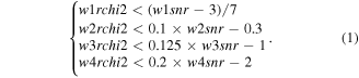
Though this set of equations is very effective in suppressing contamination from fake AllWISE detections, X. P. Koenig & D. T. Leisawitz (2014) noted that it also eliminates around two-thirds of real detections in bands W3 and W4. X. P. Koenig & D. T. Leisawitz (2014) thus changed their criteria to raise the retrieval rate in the W3 and W4 bands, at the cost of allowing more fake detections. We decide that instead of adopting this changed criteria, we select sources that either:
1. have AllWISE photometry with non-null photometric uncertainty, R ≥ 0.5 from G. Marton et al. (2019), and meet the criteria presented in Equation (1), or
2. have existing Spitzer photometry (IRAC 1-4 and MIPS1 bands with non-null photometric uncertainty) that can be used as an alternative.
We have thus only used AllWISE photometry when catalog parameters meet a number of strict requirements, and opted to search for Spitzer photometry in cases where the requirements are not met. The Spitzer photometry is acquired using the VizieR Photometry viewer tool10 with a Python interface,11 using a search radius of 2.”
We ultimately select 16 YSOs for our current sample. Nine YSOs have usable AllWISE photometry determined with our criteria, and 15 of them have published Spitzer photometry. We use photometry from the c2d (Cores to Planet-forming Disks) Spitzer Legacy Program when available (N. J. I. Evans et al. 2003; C2D Team 2020), and use alternatives otherwise, as listed in Table 1. To classify the YSOs in our sample, we use the 4-class system introduced by T. P. Greene et al. (1994), which classifies via the spectral index α; essentially the slope of the SED between ∼2 and 20 µm:

To estimate α, we fit a line by least-squares fitting to the available AllWISE and/or Spitzer photometry. We then classify α with the cutoffs presented in T. P. Greene et al. (1994):
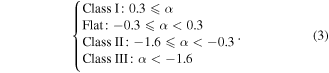
Information related to the VIRUS observations of each star is presented in Table 10 in Appendix A. Table 1 contains the YSO likelihood LY and the AllWISE validity likelihood R obtained from G. Marton et al. (2019), the classification and region for each object, the photometry used in determining each classification12 , and the name of the object in the SIMBAD database. We find 12 of the stars are class II, and four are class III. Among them, Object 10 (EM* LkHA 351) is classified as class II but its spectral index α very nearly places it in the class III category. Object 3 (2MASS J20580138+4345201) is also considered class II, but is almost in the “Flat” category. Though it has a class II SED, the spectrum of Object 16 (ATO J052.3580+31.4444) could not be fit by a model of an accreting YSO, nor did it exhibit the Balmer emission lines expected of an accreting YSO. These two issues are discussed in Sections 4 and 6, respectively. Ultimately, this object was not included in the results (i.e., in Tables 5 and 6). By visual inspection, none of the objects had SEDs that resembled transition disk YSOs.
Table 1. Photometry and Classification Information for the Total Sample
| ID | SIMBAD Name | LYa | Rb | AllWISE ID | Spitzer Source | α | Class | Region | Note |
|---|---|---|---|---|---|---|---|---|---|
| 1 | 2MASS J21523325+4710505 | 0.9354 | 0.456 | 2 | −0.84 | II | IC 5146 | ||
| 2 | 2MASS J21533310+4716092 | 0.9798 | 0.422 | 2 | −1.09 | II | IC 5146 | ||
| 3 | 2MASS J20580138+4345201 | 0.9966 | 0.56 | J205801.37+434520.1 | 3 | −0.32 | II | NGC 7000 | |
| 4 | EM* LkHA 188 | 0.9972 | 0.568 | J205823.80+435311.3 | 3 | −0.8 | II | NGC 7000 | |
| 5 | 2MASS J18300610+0106170 | 0.9996 | 0.5 | J183006.10+010616.8 | 1 | −0.71 | II | Serpens | |
| 6 | 2MASS J18295618+0110574 | 0.8058 | 0.448 | 1 | −2.55 | III | Serpens | ||
| 7 | V* V776 Ori | 0.8752 | 0.388 | 5 | −2.22 | III | Orion | ||
| 8 | CVSO 1897 | 0.9888 | 0.51 | J054015.13-005726.6 | −0.87 | II | Orion | ||
| 9 | [HL2013] 052.17673+30.49810 | 0.9996 | 0.55 | J032842.43+302953.0 | 1 | −0.82 | II | Perseus | |
| 10 | EM* LkHA 351 | 0.997 | 0.596 | 1 | −1.56 | II | NGC 1333 | ||
| 11 | 2MASS J03285101+3118184 | 0.9996 | 0.644 | J032851.03+311818.3 | 1 | −0.61 | II | NGC 1333 | |
| 12 | 2MASS J03283651+3119289 | 0.9004 | 0.21 | 1, 4 | −2.58 | III | NGC 1333 | ND | |
| 13 | 2MASS J03292815+3116285 | 0.9346 | 0.264 | 1, 4 | −2.5 | III | NGC 1333 | ND | |
| 14 | 2MASS J03284782+3116552 | 0.9956 | 0.638 | J032847.83+311655.0 | 1 | −0.91 | II | NGC 1333 | |
| 15 | 2MASS J03285216+3122453 | 1.0 | 0.506 | J032852.16+312245.1 | 1 | −1.04 | II | NGC 1333 | |
| 16 | ATO J052.3580+31.4444 | 0.9972 | 0.55 | J032925.92+312640.0 | 1 | −0.69 | II | NGC 1333 |
Notes. ND: Object has MIPS1 photometry from Table 2 of H. Y. A. Meng et al. (2017) with the flag “Not Individually Detected”. aLY: the YSO likelihood in G. Marton et al. (2019). bR: the AllWISE validity likelihood in G. Marton et al. (2019).References. (1) N. J. I. Evans et al. (2003); (2) P. M. Harvey et al. (2008); (3) L. M. Rebull et al. (2011); (4) H. Y. A. Meng et al. (2017); (5) D. Cornu & J. Montillaud (2021).
Download table as: ASCIITypeset image
The four class III objects are 6, 7, 12, and 13. Two of these objects, 12 and 13 (2MASS J03283651+3119289 and 2MASS J03292815+3116285), have Spitzer IRAC and MIPS1 photometry obtained from separate catalogs since their MIPS1 photometry could only be found exclusively in Table 2 of H. Y. A. Meng et al. (2017). For both these objects, the MIPS1 photometry is labeled as “Not Individually Detected” by H. Y. A. Meng et al. (2017). Despite the dubious nature of their MIPS1 detections, we nonetheless include these two objects because their spectra confirm that they are young stars and because the MIPS1 photometry is not used for anything beyond categorizing the YSOs as class III.
4. Analysis: Bayesian Fitting to the Continuum
In Section 3 we identified a sample set of YSO spectra, for which we now develop a procedure to fit a multicomponent YSO model. The goal is to acquire accretion luminosities Lacc of our class II sample using the “direct” method (fitting a model of excess continuum emission to the spectrum) with a Bayesian approach. We have written our procedure into a publicly available Python code called nuts-for-ysos. We first outline the methodology of nuts-for-ysos in Sections 4.1, 4.2, and 4.3. We then discuss in Section 4.4 the specific requirements of nuts-for-ysos for inputted YSO spectra, and which parts of the analysis can be customized by the user.
4.1. The Model
The continuum of a YSO spectrum in the UV and optical range is mainly affected by two different phenomena, which need to be modeled simultaneously. Accretion from its circumstellar disk causes a YSO to display stronger continuum emission in the blue end of its spectrum, along with emission lines and a veiling of its photospheric absorption lines. On the other hand, flux from the YSO may be extinguished by foreground material, local material within the surrounding molecular cloud, and material within its own circumstellar disk. This extinction subdues the blue part of the spectrum. The two phenomena thus have opposite effects on the perceived temperature of the star, making them difficult to disentangle (C. F. Manara et al. 2013a). We therefore use a model that incorporates both the accretion and extinction simultaneously so that these dual effects can be considered when determining the stellar properties. Since we are fitting the U-band region of the spectrum, any contribution from the protoplanetary disk itself is negligible, and we can ignore that component in the modeling.
Accretion Spectrum. We use a slab of isothermal hydrogen in local thermodynamic equilibrium (LTE), including emission from both H and H−, to model the excess continuum emission from accretion. This approach has been used numerous times in the past to derive accretion luminosities (e.g., J. A. Valenti et al. 1993; G. J. Herczeg & L. A. Hillenbrand 2008; E. Rigliaco et al. 2012; C. F. Manara et al. 2013a; J. M. Alcalá et al. 2014, 2017). We take the equations for the slab model from C. F. Manara (2014). The slab model by itself has three parameters: electron temperature (Tslab), electron density (ne), and optical depth at λ = 300 nm (τ0). This model was originally developed to describe particles transversing a boundary layer between the disk and stellar surface (D. Lynden-Bell & J. E. Pringle 1974). This is contrary to the more current paradigm of magnetospheric accretion producing shocks on the stellar surface, as in models like that of N. Calvet & E. Gullbring (1998). Nonetheless, the slab model is still oftentimes trusted as a relatively simple empirical way to determine a bolometric correction for the accretion luminosity Lacc, even if the three parameters Tslab, ne, and τ0 themselves do not have a physical basis. Further justification for using the slab model is discussed in Section 7.1 and can also be found in C. F. Manara (2014).
Photospheric Templates. While the slab model represents the excess emission due to accretion, the photospheric contribution to a YSO spectrum can be represented by a class III spectrum of the same spectral type. Modeling the photosphere of an accreting YSO (the “target”) using a nonaccreting YSO (the “template”) is considered a better approach than using a main-sequence star. This is because it better captures the effects of elevated chromospheric activity and the altered surface gravity of YSOs compared to field dwarfs, which makes for an overall more accurate representation of the photosphere (C. F. Manara et al. 2013a). We use a total of 23 class III photospheric templates taken from C. F. Manara et al. (2013b) and C. F. Manara et al. (2017a). These class III YSOs were chosen by the authors because they have an AV ≈ 0. The spectra were acquired with the ESO VLT/X-shooter spectrograph (R ∼ 4000–17000, depending on wavelength and slit width; J. Vernet et al. 2011), and have been convolved with a Gaussian to match the lower VIRUS resolution. The templates range in spectral type from G5–M9.5, with the most thorough sample (at least one template per SpT) ranging from G8–M6.5. Each of these templates has a Teff estimated from its SpT, following the same SpT-Teff scale as in C. F. Manara et al. (2013b) and C. F. Manara et al. (2017a). For the earlier templates up to M0, the scale uses the relation from S. J. Kenyon & L. Hartmann (1995) and for later templates, the relation from K. L. Luhman et al. (2003). The corresponding distances, luminosities, and uncertainty on the luminosity (estimated 0.2 dex) for the templates we take directly from C. F. Manara et al. (2013b) and C. F. Manara et al. (2017a). As discussed in Section 4.3.1, the flux for each template is rescaled such that the NUTS sampler can easily interpolate between them. The complete list of photospheric templates used in this paper is provided in Table 2. Recently, 19 more de-reddened class III photospheric templates were introduced by R. A. B. Claes et al. (2024) to make a grid of 57 templates in total. R. A. B. Claes et al. (2024) also includes updated estimates for the luminosity L* and the effective temperature Teff, using the SpT-Teff scale from G. J. Herczeg & L. A. Hillenbrand (2014). These values for L* and Teff are different from the values we had taken from C. F. Manara et al. (2013b) and C. F. Manara et al. (2017a). Moreover, R. A. B. Claes et al. (2024) included uncertainties on SpT, luminosity, and distance individual to each object. While these new templates were not involved in our analysis, nuts-for-ysos is capable of using the updated template library, which can then be utilized in future works. R. A. B. Claes et al. (2024) also included an interpolation procedure between the templates of this enhanced grid, which we discuss in Section 4.3.1.
Table 2. Photospheric Templates and Corresponding Data Taken from C. F. Manara et al. (2013b) and C. F. Manara et al. (2017a)
| Name | SpT | Teff | log(L⋆/Lsun) | Distance (pc) | Source |
|---|---|---|---|---|---|
| RXJ0445.8+1556 | G5 | 5770 | 0.485 | 140 | 2 |
| RXJ1508.6-4423 | G8 | 5520 | 0.043 | 150 | 2 |
| RXJ1526.0-4501 | G9 | 5410 | −0.061 | 150 | 2 |
| RXJ1515.8-3331 | K0.5 | 5050 | 0.098 | 150 | 2 |
| RXJ0457.5+2014 | K1 | 5000 | −0.15 | 140 | 2 |
| RXJ0438.6+1546 | K2 | 4900 | −0.024 | 140 | 2 |
| RXJ1547.7-4018 | K3 | 4730 | −0.081 | 150 | 2 |
| RXJ1538.6-3916 | K4 | 4590 | −0.217 | 150 | 2 |
| TWA 9A | K5 | 4350 | −0.61 | 68 | 1 |
| RXJ1540.7-3756 | K6 | 4205 | −0.405 | 150 | 2 |
| TWA 6 | K7 | 4060 | −0.96 | 51 | 1 |
| TWA 25 | M0 | 3850 | −0.61 | 54 | 1 |
| TWA 14 | M0.5 | 3780 | −0.83 | 96 | 1 |
| TWA 13B | M1 | 3705 | −0.7 | 59 | 1 |
| TWA 2A | M2 | 3560 | −0.48 | 47 | 1 |
| TWA 7 | M3 | 3415 | −1.14 | 28 | 1 |
| Sz121 | M4 | 3270 | −0.34 | 200 | 1 |
| SO797 | M4.5 | 3200 | −1.26 | 360 | 1 |
| SO641 | M5 | 3125 | −1.53 | 360 | 1 |
| SO999 | M5.5 | 3060 | −1.28 | 360 | 1 |
| Par-Lup3-1 | M6.5 | 2935 | −1.18 | 200 | 1 |
| CHSM17173 | M8 | 2710 | −1.993 | 160 | 2 |
| TWA 26 | M9 | 2400 | −2.7 | 42 | 1 |
References–(1) C. F. Manara et al. (2013b); (2) C. F. Manara et al. (2017a)
Download table as: ASCIITypeset image
Combined Model. The slab and the photospheric template are separately scaled and then added together. The reason for the scaling is to match the raw flux of the model to the flux of each target, which has its own inherent distance and luminosity. Then, the entire model spectrum is reddened to match the extinction of the target. We use the reddening law presented in J. A. Cardelli et al. (1989) with RV = 3.1. There are thus a total of seven parameters involved in the model: the three slab parameters (Tslab, ne, and τ0), the scale factor of the slab (Kslab), the effective temperature Teff of the photospheric template, the scaling of the photospheric template (Kphot), and the overall extinction of the model (AV).
4.2. Criteria Used in Fitting
As in C. F. Manara et al. (2013a), we do not explicitly fit the entire target YSO spectrum but instead choose certain features of the spectrum that the model fitting attempts to match. The nuts-for-ysos code allows the user to customize which features of the spectrum to use. The tool is by default capable of computing several different “types” of spectral features: individual flux values, slopes, ratios, and photometric magnitudes. The number, types, and wavelength ranges of these features can be changed by the user as desired. For our particular work with VIRUS spectra, we chose features that sample both bluer parts of the spectrum dominated by accretion emission (around the Balmer Jump) and redder parts of the spectrum dominated by photospheric emission. The chosen features deliberately avoid wavelengths with strong emission lines. The emission lines of an accreting YSO are not replicated by the simple model we use, and separately modeling these emission lines would be a more complicated process. The chosen features include the slope of the Balmer continuum between ∼3500 and ∼3600 Å, the slope of the Paschen continuum between ∼3980 and ∼4790 Å, the slope of the continuum between ∼5060 and ∼5420 Å, and the value of the continuum at several locations (∼3600 Å, ∼3860 Å, ∼4020 Å, ∼4610 Å, and ∼5480 Å). Overall, these features are similar to those used in C. F. Manara et al. (2013a). However, C. F. Manara et al. (2013a) used targets from the ESO VLT/X-shooter spectrograph, which has a larger wavelength region available for fitting spectral features. Instead, our spectrum occupies the shorter-wavelength region of VIRUS. We attempt to make up for the lack of VIRUS coverage from ∼5500 to ∼7150 Å by instead using photometry (an approach originally suggested in C. F. Manara et al. 2013a). We compute synthetic Pan-STARRS r and i magnitudes for models. These synthetic magnitudes are included as features to be compared to the actual Pan-STARRS DR1 r and i magnitudes of the targets. Because this photometry is nonsimultaneous with the spectrum, and because of the inherent variability of YSOs, we assign conservative uncertainties of 0.2 mag to the Pan-STARRS r and i magnitudes when performing the fitting. The exact wavelength ranges for these 11 features are reported in Table 3. Only these features are used when fitting the model to the target spectrum. It should be emphasized that the process for fitting the model attempts to fit only the continuum and not the emission lines, a practice consistent with previous similar works. This is most evident near the higher-level Balmer lines, where the spacing between lines becomes small and the superimposed lines form a pseudo-continuum for which the model does not account.
Table 3. Spectral Features Used in Fitting the Total Model to Each Target Spectrum
| Name | Wavelength Range (Å) |
|---|---|
| Slope of Balmer continuum | mean[3580:3600]-mean[3504:3524] |
| Slope of Paschen continuum | mean[4770:4790]-mean[3980:4000] |
| Slope ∼508 nm to ∼541 nm | mean[5390:5424]-mean[5060:5100] |
| Continuum at ∼360 nm | mean[3580:3620] |
| Continuum at ∼386 nm | mean[3850:3870] |
| Continuum at ∼402 nm | mean[4000:4030] |
| Continuum at ∼461 nm | mean[4596:4624] |
| Continuum at ∼511 nm | mean[5090:5130] |
| Continuum at ∼548 nm | mean[5470:5490] |
| Pan-STARRS r magnitude | Pan-STARRS r filter [5200:7100] |
| Pan-STARRS i magnitude | Pan-STARRS i filter [6700:8400] |
Download table as: ASCIITypeset image
4.3. Initializing the Bayesian Fit
We use the Python package PyMC (J. Salvatier et al. 2016) to implement a Bayesian process for fitting the total model to each target spectrum. Within PyMC, we use the No U-Turn Sampler (NUTS) with 16 chains, each having a length of 2000. We set target_accept = 0.99, so that the sampler takes very small steps. We used NUTS because for a system with significant parameter correlations such as ours, a Hamiltonian-based Monte Carlo algorithm like NUTS is more efficient than the Metropolis–Hastings algorithm or Gibbs sampling (M. D. Hoffman & A. Gelman 2014).
To reduce the burn-in time, a starting point for the sampler is determined using a least-squares optimization. In finding the starting point, we attempt to match the spectral features listed in Table 3 by minimizing a likelihood function similar to a χ2 function. This  function was first introduced in C. F. Manara et al. (2013a) and is as follows:

where fobs is the feature from the VIRUS spectrum, σobs is the respective uncertainty, and f is the same feature predicted the composite model. After the starting point for each parameter is found, it is used as the initial point for the chains of the NUTS sampler.
4.3.1. Interpolating between Photospheric Templates
NUTS requires each parameter in the model to have a continuous range, because it is a gradient-based sampler. NUTS takes the gradient of the likelihood with respect to each parameter, to reach convergence faster than other sampling methods (M. D. Hoffman & A. Gelman 2014). Six out of the seven total model parameters are inherently continuous, but Teff is not, because we rely only on a set of 23 discrete photospheric templates of various spectral types. We thus made Teff a continuous parameter by having the sampler linearly interpolate between photospheric templates. Each of the class III photospheric templates comes from real observations rather than simulation, and so each has an (unspecified) uncertainty on its stellar distance provided in C. F. Manara et al. (2013b) or C. F. Manara et al. (2017a). This introduces scatter in the perceived relative brightnesses between templates. For the sampler to smoothly interpolate between templates, we decided to scale the flux of each template so the templates are at the same distance, and then slightly rescale both the templates and their respective luminosities L*,phot so that the brightness from each template would smoothly and monotonically increase with Teff. We do so by forcing the median fluxes from 4500 to 5500 Å of each template to follow a fourth-degree polynomial fitted to the original medians. Figure 1 shows these original medians plotted against Teff, with the best-fit polynomial overlaid as a dashed line. These adjustments ultimately give the sampler an easier set of templates to interpolate between without fundamentally changing the nature of the results. Without this cleaning of the templates, we would not have been able to make Teff a continuous parameter in the model and instead would have needed to make an ad hoc selection of a template before the rest of the model-fitting process.
A similar methodology has been used by R. A. B. Claes et al. (2024) to interpolate between their grid of 57 class III photospheric templates. They first normalized their class III spectra to factor out the individual distances to each star. They then computed the median fluxes of the spectra within multiple wavelength ranges. Next, they performed nonparametric local polynomial fits to the medians as a function of SpT. The smooth curve resulting from each fit then served as a basis for an interpolable set, such that the grid of templates could be made as well-sampled as needed. Within the polynomial fitting procedure, they also account for uncertainties in the median fluxes, the extinction, and spectral type of each template. They do this by repeating the polynomial fit over 1000 Monte Carlo iterations with the error terms sampled from Gaussian distributions. The result of this process is that each interpolated template has an uncertainty in the spectral flux. This inclusion of uncertainty within the interpolation is an important addition, which was not in our work. In our work, we simply incorporated uncertainties of AV and Teff directly into the Bayesian inference of the parameters. However, propagating uncertainty during the template interpolation stage could be particularly relevant when using the late-M spectral type class III templates, which generally have the lowest SNRs in the grid. The interpolation procedure of R. A. B. Claes et al. (2024) is available through their FRAPPE tool on Github.13 While our own interpolation did not use this approach, nuts-for-ysos has recently been updated with a new version that gives the NUTS sampler the ability to include uncertainties in the spectral flux of an inputted template grid, such as those acquired from FRAPPE.
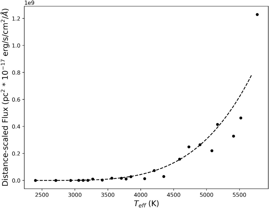
Figure 1. The median values of each photospheric template flux, after being multiplied by its squared distance. A fourth-degree polynomial is fit to the medians, and the template fluxes and respective luminosities are then rescaled to match this polynomial.
Download figure:
Standard image High-resolution image4.3.2. Priors
After making the adjustment so the Teff parameter is continuous rather than discrete, we are then able to create priors for every component of the YSO model. A schematic diagram is presented in Figure 2 showing how each prior contributes to the model. The priors associated with the slab model are bounded within a mostly typical range of parameter space: Tslab ranges from 5000–11,000 K, ne ranges from 1010–1016 cm−3, and τ0 ranges from 0.01–5.0. The Tslab and τ0 priors are uniform distributions, and ne is a uniform distribution in logarithmic space. The priors for Kslab and Kphot are set as Half-Flat distributions, constraining them to be above zero. The AV prior is a uniform distribution bounded between 0 and 10.
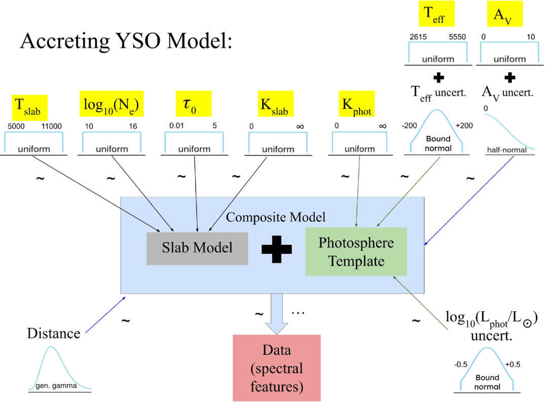
Figure 2. A diagram illustrating the components of the YSO model. Parameters that are fitted for are highlighted in yellow. The shape of each prior is shown using Kruschke-style plots. Each prior has a color-coded arrow indicating whether it belongs to the slab portion, the photospheric portion, or to the entire composite model (black, green, and blue, respectively).
Download figure:
Standard image High-resolution imageTable 4. Priors Used
| Name of Prior | Distribution Type | Lower Bound | Upper Bound |
|---|---|---|---|
| Tslab | Uniform | 5000K | 11000K |
| log(ne) | Uniform | 1010cm−3 | 1016cm−3 |
| τ0 | Uniform | 0.01 | 5.0 |
| Kslab | Half-Flat | 0 | ∞ |
| Kphot | Half-Flat | 0 | ∞ |
| Teff | Uniform | 2615 K | 5550 K |
| Teff Uncert | Bounded Normal (μ = 0K, σ = 100K) | −200K | 200K |
| AV | Uniform | 0 | 10 |
| Distance dobs | GGDa | 0 pc | ∞ pc |
| Phot. template AV | Half-Normal (σ = 0.167) | 0 | ∞ |
| Phot. template log(L*,phot/L⊙) Uncert | Bounded Normal (μ = 0, σ = 0.2) | −0.5 | 0.5 |
Note. aMedian, 16th percentile, and 84th percentile of generalized gamma distribution defined for each target using the distance values in Table 5.
Download table as: ASCIITypeset image
The benefit of a Bayesian model for the fitting is that systemic uncertainties in the photospheric templates can be seamlessly integrated into the model. For example, the templates have an uncertainty in their spectral type of roughly 1 subclass for K-type stars, and half a subclass for M-type stars (C. F. Manara et al. 2013b; C. F. Manara et al. 2017a), which we translate into an uncertainty in Teff of 100 K. The prior for Teff by itself is set to be a Uniform prior, bound between 2615 and 5550 K (roughly SpTs M8.5 to G8), but a Normal prior centered on 0K with σ = 100 K is then added to this, to reflect the uncertainty in Teff of the photospheric templates. However, the Teff uncertainty can only extend to the extrema of available templates (SpTs M9 and G5), beyond which we are unable to generate a model. We therefore bound the Teff uncertainty prior to be within ±200K.
Additionally, the photospheric templates are uncertain in their extinction; although the templates were selected by C. F. Manara et al. (2013b) and C. F. Manara et al. (2017a) to have AV close to zero, it is more accurate to include a possibility of nonzero extinction. According to C. F. Manara et al. (2017a), all templates compared to BT-Settl models (F. Allard et al. 2011) have an AV < 0.5 mag, with the possibility of AV = 0 mag being within 3σ at most. We add a Half-Normal prior centered on 0 with σ = 0.5/3 to the uniform AV prior, to represent this uncertainty on AV.
We also include other uncertainties not directly related to a fitted parameter. The photospheric templates have an uncertainty in their luminosity L*,phot, given by C. F. Manara et al. (2013b) to be 0.2 dex. We represent this uncertainty with a Normal prior in log space, centered on 0 with σ = 0.2. For the distance to each target YSO, the catalog associated with C. A. L. Bailer-Jones et al. (2021) provides the median, 16th percentile, and 84th percentile of a posterior probability distribution. C. A. L. Bailer-Jones et al. (2021) used a generalized gamma distribution (GGD) as a prior when computing the “geometric distances” we used. We thus choose to represent the distance to each target YSO as a GGD, defined using the median, 16th percentile, and 84th percentile. Table 4 summarizes all of the priors.
4.4. The nuts-for-ysos Workflow
The nuts-for-ysos package incorporates the Bayesian analysis described throughout Section 4. The code has been written to also be compatible with YSO spectra obtained by other instruments other than VIRUS. The inputted YSO spectrum can be of a higher resolution than that of VIRUS, but it must be of the same or lower resolution than the Class III templates, and must occupy a wavelength range covered by the Class III templates (for example, between 3300.0 Å and 10189.0 Å if using the UV and optical Class III templates from X-Shooter). The user can customize several aspects of the analysis. The grid of interpolable Class III templates can be changed from the default grid of templates listed in Table 2. For example, the new grid of templates presented in R. A. B. Claes et al. (2024) is better sampled in SpT and can be substituted within nuts-for-ysos. The only requirement for the templates themselves is that the wavelengths of the template spectra are no lower than 500.0 Å or higher than 25000.0 Å. As mentioned in Section 4.2, the features for which the model is evaluated can also be altered within nuts-for-ysos. The tool is by default capable of computing individual flux values, slopes, ratios, and photometric magnitudes from spectra. The number, types, and wavelength ranges of these features can be changed by the user as desired. As an example, we tested nuts-for-ysos with several low-resolution class II YSO spectra among the HST ULYSSES survey (J. Roman-Duval et al. 2020). 14 Specifically, we fit the model to data from the R ∼ 500 STIS G430L and G750L gratings. We did so between 3300Å and 6000Å, using the same Class III templates in Table 2 and using the same features as in Table 3, with three additional features included at ∼3310 Å, ∼5850 Å, and ∼6000 Å. We found the code runs successfully, and we show in Figure 3 an example fit for the Class II YSO Sz97. We performed compatibility tests of nuts-for-ysos with X-Shooter data of several Class II YSOs from J. M. Alcalá et al. (2014) and J. M. Alcalá et al. (2017) as well. Version 1.1 of nuts-for-ysos is available on GitHub15 and on Zenodo (L. H. Willett et al. 2024).
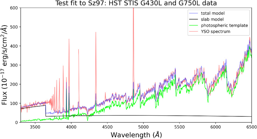
Figure 3. The median model fit resulting from testing nuts-for-ysos on HST STIS G430L and G750L data of Sz97, considering 14 different continuum features between ∼3300 Å and ∼6000 Å.
Download figure:
Standard image High-resolution image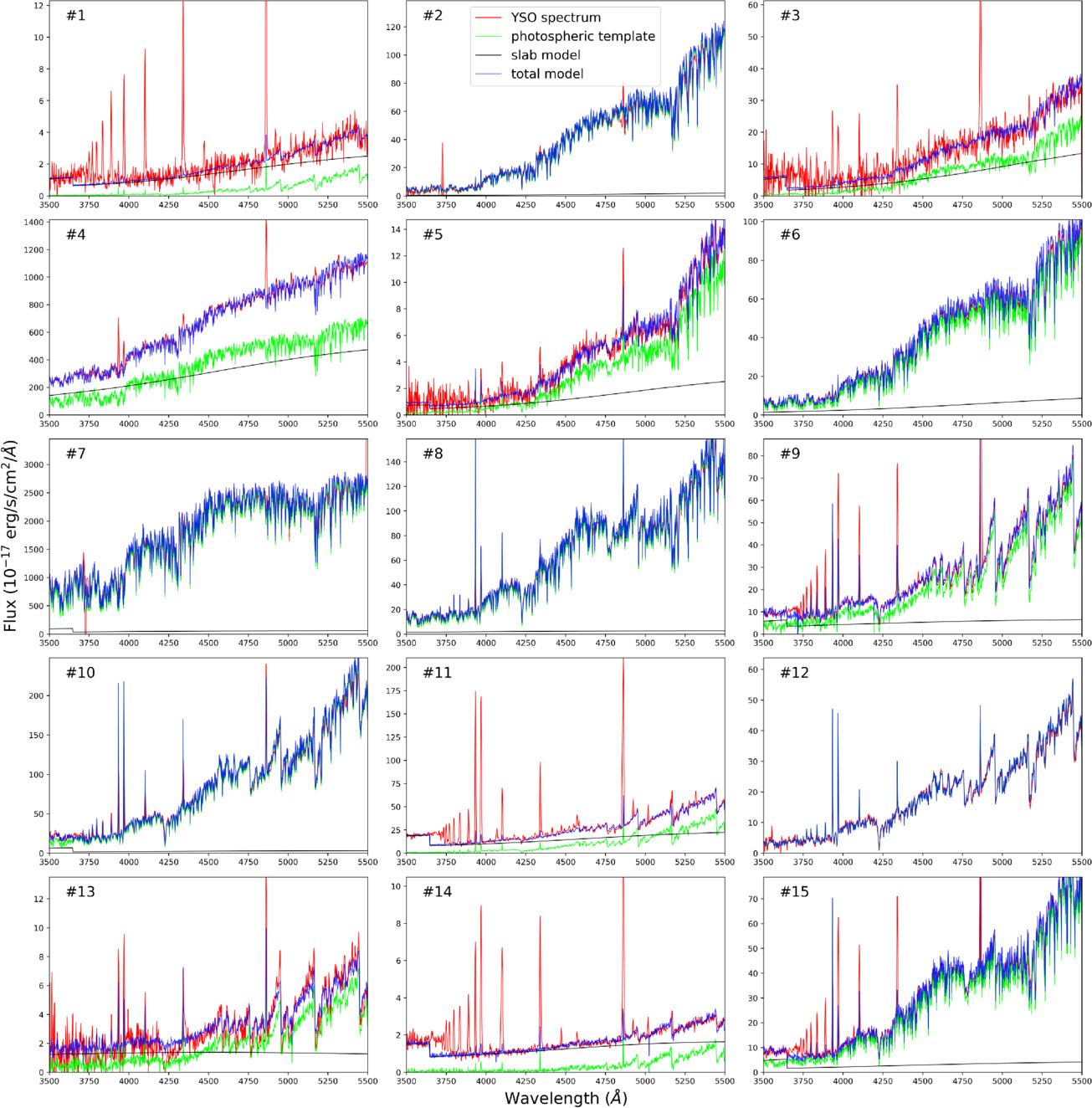
Figure 4. The YSO model fit to VIRUS spectra of class II and class III YSOs. On the top left of each plot is the object ID originating in Tables 1 and 10. The VIRUS spectrum (red) has a model fit to its continuum (blue), which is the sum of the hydrogen accretion slab (black) and the photospheric template (green).
Download figure:
Standard image High-resolution image5. Accretion Model Fit Results
We check for convergence of each fit using the Gelman-Rubin statistic, by requiring  ≤ 1.1 (A. Gelman & D. B. Rubin 1992) for every parameter. To mitigate autocorrelation, we only use every 20th value in each parameter posterior outputted by PyMC to compute further results. Since we ran 16 chains with length 2000 each, the original posterior has a length of 32,000, and the new thinned posterior has length of 1600.
The composite model can have a Teff of at least 2615 K and at most 5550 K. We encountered two cases in which the fitted model to a target from our sample had an effective temperature on the edge of these boundaries. Object 13 (2MASS J03292815+3116285), a class III YSO, was found to have a Teff posterior that peaks at ∼2600 K and is cut off for lower temperatures. Similarly, for Object 4 (EM* LkHA 188), a class II YSO, we found a Teff posterior that peaks at ∼5500K and is cut off for higher temperatures. Because the sampler was unable to explore the entirety of the plausible model parameter space for these two objects, we take their Teff to be upper and lower limits, respectively. The results for their other parameters are taken to only be approximate throughout further analysis.
Object 16 (ATO J052.3580+31.4444) was the only star for which we were unable to fit an accretion model, a finding that was briefly previewed at the end of the Sample Selection section (Section 3). This object has seemed to be a YSO in some ways, as it belongs to NGC1333 and has a class II SED. However, we found that our process was unable to plausibly fit an accretion model to the spectrum of Object 16. The spectrum also appears to have Balmer lines that are in absorption rather than emission, as discussed in Section 6. We were only able to fit a model of a reddened class III template having Teff ≈ 5500 K and AV ≈ 3.0. A plot of the data and model is shown in Figure 5.
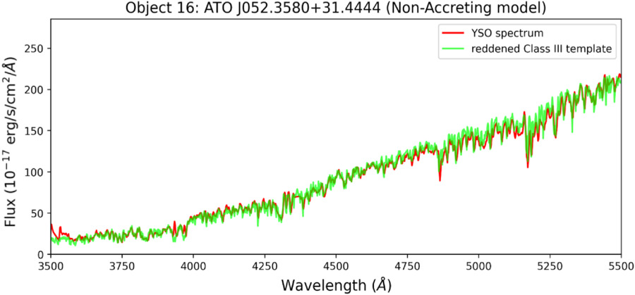
Figure 5. Object 16 (ATO J052.3580+31.4444), the one YSO in our current sample for which we were unable to fit a model including accretion. Instead, we fit the spectrum (red) with only a reddened Class III template (green) having Teff ≈ 5500K and AV ≈ 3.2.
Download figure:
Standard image High-resolution imageFor the rest of the objects we were successful in fitting a model of an accreting YSO that converged and explored the full plausible range of Teff. Plots of the median model fits for these 15 objects are shown in Figure 4. Figures 21–50 in Appendix B illustrate the full set of results for the 15 objects. This includes all median model fits, and underneath are also plots of probability distributions for each of the model parameters. For each object, a corner plot of the model parameters is also shown, as discussed in Section 5.2.
We find that in general, the least-constrained parameters tend to be those associated with the slab portion of the model. This is especially true of the electron density ne, which has a posterior sometimes occupying a flat or nearly flat probability distribution in logarithmic space. The posterior probability distributions of slab parameters Tslab, ne, and τ0 also sometimes appear to peak at or near the bounds of their uniform priors; however, extending the bounds on these priors into more extreme territory was often found not to reveal any sudden dropoff in probability. Other model parameters Kphot, Teff, and AV are more constrained and tend to have posterior probability distributions that are more Gaussian in appearance. In Section 7 we discuss the posteriors and their correlations in more detail.
5.1. Discerning Upper Limits on Accretion
In objects that appear to have a minimal slab component in the model fit (e.g., Objects 8, 10, and 12, as seen in Figures 35, 39, and 43 of Appendix B), there is an additional technicality that needs to be considered. The Kslab posterior reaches very low values for these objects (for example, log(106*Kslab) ∼ −5 for Object 12), but the lower bound for the uniform Kslab prior was set exactly to 0 in Section 4.3.2. The sampler has a small but nonnegligible step size, which keeps it from precisely reaching this Kslab = 0. We therefore must develop some way to check each object for whether the tapering of probability at low Kslab values is a legitimate property, or if it is caused by boundary behavior. We accomplish this by creating an altered Kslab prior that is uniform instead in logarithmic space. The lower bound of this prior is set to log(106*Kslab) = −10, which is much lower than any Kslab resulting from the original model fits. If fitting the model with this new Kslab prior yields a posterior that goes all the way down to –10, then this means the original model fit was affected by the lower bound of the prior. In these cases, our original model fit should only be interpreted as an upper limit on accretion. The object could be accreting, but it also might not be accreting at all. In the opposite scenario, if the object is definitely accreting, the resulting Kslab will be biased toward lower values but will still taper off in probability at approximately the same value as the original result.
Using this criteria, we find that five YSOs have slab components that should only be interpreted as upper limits: the class III objects 6, 7, and 12, and class II objects 2 and 8. Figure 6 illustrates the difference between Kslab posteriors of a YSO that is definitely accreting, albeit relatively low (Object 10), and a YSO which has an upper limit only (Object 8). For Object 10, the posterior tapers at ≈ −1 regardless of which prior is used. For Object 8, the posterior resulting from the altered prior extends all the way to the lower bound of log(106*Kslab) = −10.
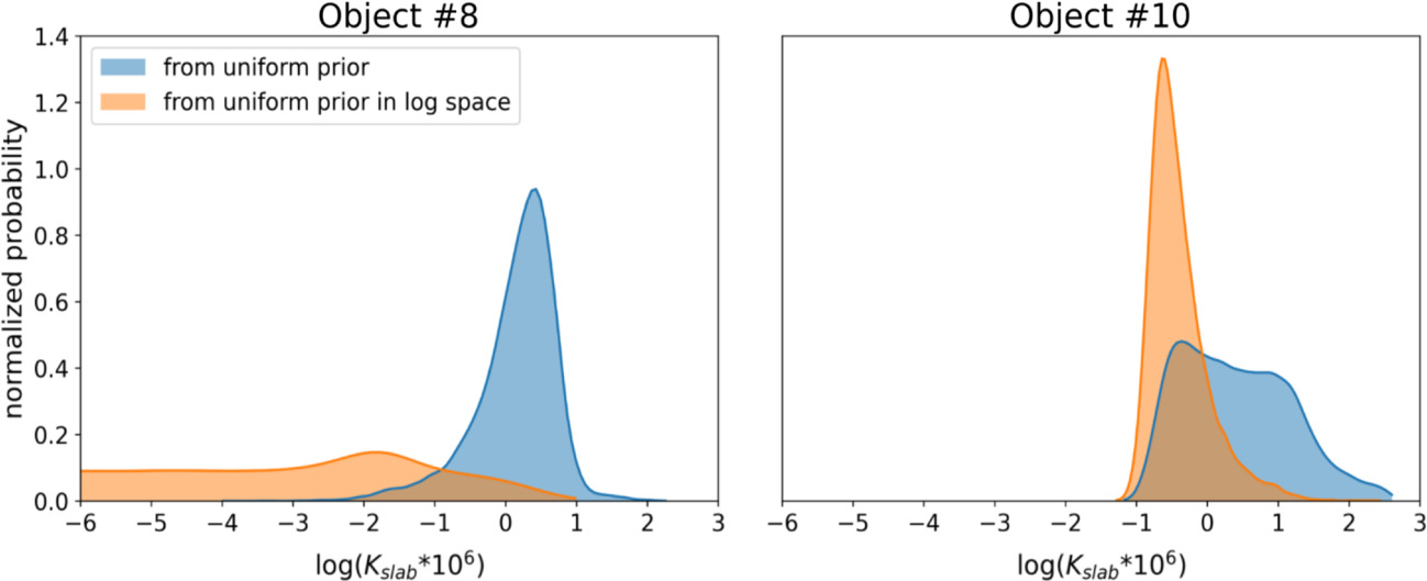
Figure 6. Comparison of Kslab posteriors (expressed as log(106*Kslab)) for Object 8 versus Object 10. In blue is the original Kslab posterior, using the uniform prior for Kslab that was introduced in Section 4.3.2 and Table 4. In orange is the posterior resulting from an altered Kslab prior that is uniform instead in logarithmic space. From this comparison, we see that Object 8 is possibly nonaccreting by virtue of having a slab component in the accretion model, which approaches zero.
Download figure:
Standard image High-resolution image5.2. Calculating Luminosity and Accretion Luminosity from Fit
The flux from accretion Facc is derived simply by integrating the hydrogen spectrum portion of the model fit (the “slab” portion) over a very wide wavelength range; we integrate from 500 Å to 25000 Å. The integration is repeated for every possible slab created by the posterior. Facc is then converted into an accretion luminosity using the relation  for a distance dobs from the target. The stellar luminosity of each target is derived using the class III template portion of the model fit (the photspheric portion). Every best-fit class III template has a precomputed luminosity L*,phot as discussed in Section 4.3.1, which can then be combined with the determined template scaling, Kphot, to calculate the stellar luminosity L* of the target. The formula is:

Since every parameter involved in these calculations occupies a probability distribution defined in advance or defined by posterior outputted by PyMC, we are essentially building probability distributions for L* and Lacc.
Table 5 lists averages and standard deviations for the most physically relevant parameters of the sample: Teff, AV, log(L*), and log(Lacc), as well as the distances to each of these targets (with their 16th and 84th percentiles included). Objects 4 and 13, for which Teff is only a lower or upper limit, have all other model parameters listed as approximate. The objects with the lowest-SNR VIRUS spectra in Table 10 of Appendix A tend to have the largest uncertainties in Teff and AV, and the largest fractional uncertainty in Kphot. These uncertainties translate into wider error bars on log(L*) and log(Lacc). For example, the class II Objects 1 and 3 (with average SNRs of 5.6 and 5.8, respectively) both have a standard deviation in log(Lacc) of σlog(Lacc) ∼ 0.5, larger than the σlog(Lacc) ∼ 0.15–0.30 found for other objects in the sample. In Table 5, we do not list numerical results for Tslab, ne, and τ0. As we briefly addressed in Section 4.1 (and discussed further in Section 7), the flux of the slab model is useful for determining Lacc, but the model itself is based on simplified physical assumptions, and so the numerical results for these three individual parameters should not be considered in great detail.
Table 5. Both Class II and Class III YSOs from the Sample, with Information on Their Distances Taken from C. A. L. Bailer-Jones et al. (2021), and Information on Temperature, Distance, Luminosity, and Accretion Luminosity Derived from the Model Fit to the Continuum
| ID | Class | dobs (pc) | dobs,L (pc) | dobs,U (pc) | Mean Teff | σTeff | Mean AV | σAV | Mean log(L*) | σlog(L*) | Mean log(Lacc) | σlog(Lacc) |
|---|---|---|---|---|---|---|---|---|---|---|---|---|
| 1 | II | 694.89 | 660.88 | 746.28 | 2971 | 220 | 2.7158 | 0.9156 | −0.2056 | 0.3459 | −1.2957 | 0.5477 |
| 2 | II | 734.37 | 720.62 | 746.51 | 4291 | 107 | 2.8836 | 0.1629 | 0.5163 | 0.1657 | ≤−1.5617 | |
| 3 | II | 785.71 | 754.77 | 814.22 | 3968 | 387 | 3.4723 | 0.786 | 0.241 | 0.268 | −0.1417 | 0.5203 |
| 4 | II | 746.32 | 737.9 | 753.86 | ≥5166 | ≈ 1.4186 | ≈ 0.5773 | ≈ 0.3249 | 0.2741 | |||
| 5 | II | 411.97 | 398.19 | 430.07 | 3761 | 116 | 3.6198 | 0.3877 | −0.3555 | 0.2052 | −1.3807 | 0.3005 |
| 6 | III | 430.93 | 424.05 | 438.52 | 4341 | 114 | 2.1424 | 0.1462 | −0.3679 | 0.1564 | ≤−1.5028 | |
| 7 | III | 347.26 | 340.54 | 352.53 | 5012 | 163 | 0.1269 | 0.0994 | −0.0044 | 0.166 | ≤−1.6016 | |
| 8 | II | 335.56 | 332.25 | 338.38 | 3582 | 98 | 0.1224 | 0.0904 | −0.6987 | 0.1687 | ≤−3.1574 | |
| 9 | II | 282 | 277.84 | 286.37 | 3060 | 93 | 0.1863 | 0.1282 | −0.5797 | 0.1889 | −2.7998 | 0.1467 |
| 10 | II | 285.52 | 283.18 | 287.5 | 3350 | 94 | 0.5525 | 0.1467 | −0.2532 | 0.1578 | −2.813 | 0.2962 |
| 11 | II | 303.16 | 297.88 | 307.58 | 3147 | 111 | 2.0873 | 0.399 | −0.0704 | 0.2079 | −1.2693 | 0.2532 |
| 12 | III | 281.19 | 275.61 | 286.59 | 3274 | 92 | 0.0824 | 0.0707 | −1.0181 | 0.1653 | ≤−6.2905 | |
| 13 | III | 297.2 | 285.6 | 308.59 | ≤2938 | ≈ 0.2679 | ≈ −1.1377 | ≈ −3.413 | ||||
| 14 | II | 308.01 | 296.58 | 321.96 | 2828 | 114 | 2.1155 | 0.2844 | −0.7414 | 0.2095 | −2.2991 | 0.177 |
| 15 | II | 286.53 | 282.49 | 289.76 | 3676 | 106 | 1.0444 | 0.2114 | −0.8576 | 0.1712 | −2.542 | 0.2611 |
Download table as: ASCIITypeset image
Appendix B (containing Figures 21–50) additionally includes corner plots of the model fit results for each object: both the parameters of the model itself, as well as log(L*) and log(Lacc). We find several correlations between parameters within the corner plots, which are discussed in Section 7. Though all corner plots are in Appendix B, we also show an example for Object 11 in Figure 7. Figure 8 shows log(Lacc) plotted against log(L*) for the 15 objects, where the error bars signify the standard deviations in log(Lacc) and in log(L*). Downward arrows indicate an upper limit on log(Lacc) and open circles indicate only an approximate result for log(Lacc) and log(L*).
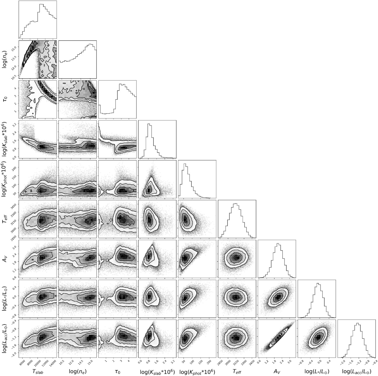
Figure 7. An example corner plot for the fit of an accreting YSO model to the spectrum of Object 11 (2MASS J03285101+3118184). Included are the model parameters as well as the log(L*) and log(Lacc) posteriors. The corner plots for all fits are given in Appendix B.
Download figure:
Standard image High-resolution image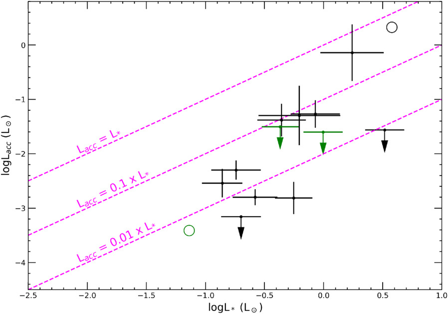
Figure 8. Plot of log(Lacc) vs. log(L*) for the class II and class III YSO targets. Class II YSOs are plotted in black, and the class III objects are plotted in green. Upper limits on logLacc are denoted with downward arrows instead of error bars. Object 12 has an upper limit for log(Lacc), but it is so low ( ≈ −6.3) that it falls below the plot limits. Object 4 is shown as a black open circle, and Object 13 is shown as a green open circle. These two objects only have upper or lower limits on Teff, as explained in Section 5, so their L* and Lacc values are taken to be approximate.
Download figure:
Standard image High-resolution image5.3. Estimating the Mass Posterior
We estimate masses for the class II and class III sample by interpolating pre-main-sequence (PMS) evolutionary models. Each object has a posterior outputted by PyMC for Teff and L*, which can be fed directly into an interpolation of evolutionary models to generate a probability distribution for the stellar mass M⋆. We interpolate two sets of PMS models, from I. Baraffe et al. (2015) and L. Siess et al. (2000). The I. Baraffe et al. (2015) models are available for masses ≤1.4M⊙ and ages ≥ 0.5 Myr. The L. Siess et al. (2000) models extends to younger ages and to a higher mass of 7M⊙, but the lowest mass available is 0.1M⊙. An HR diagram for all of the targets is plotted in Figures 9 and 10 with the I. Baraffe et al. (2015) and L. Siess et al. (2000) tracks, respectively.
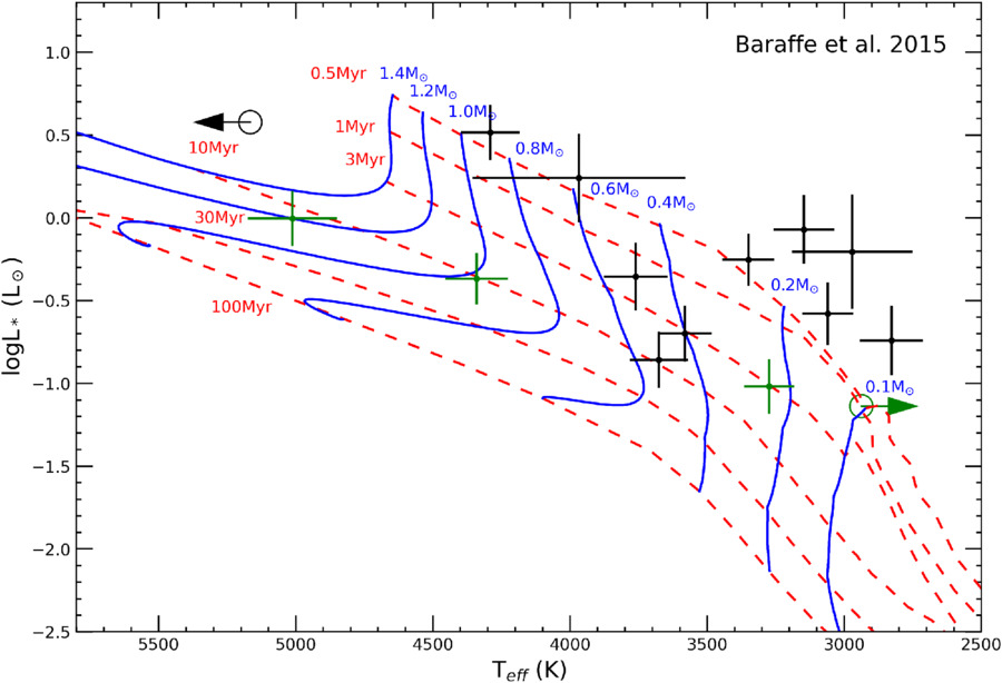
Figure 9. Hertzsprung–Russell diagram for the total sample, plotted over evolutionary tracks (blue lines) and isochrones (dashed red lines) from I. Baraffe et al. (2015). Class II YSOs are plotted in black, and class III YSOs are plotted in green. Objects 4 and 13 have only approximate L* and are therefore shown as open circles, with arrows to signify their respective lower and upper limits on Teff.
Download figure:
Standard image High-resolution image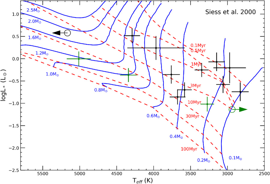
Figure 10. Hertzsprung–Russell diagram for the total sample, plotted over evolutionary tracks (blue lines) and isochrones (dashed red lines) from L. Siess et al. (2000). Plotting conventions are the same as in Figure 9.
Download figure:
Standard image High-resolution imageFor the I. Baraffe et al. (2015) tracks, there are a number of objects (all class II) that lie above the youngest isochrone. We use a nearest interpolation for these objects, as opposed to linear interpolation for the rest. When determining which mass track a data point is nearest to on the HR diagram, we create a metric where 1 dex in log(L*) scales to 1000K in Teff. This scaling matches the ratio of the full ranges in log(L*) and Teff covered by the I. Baraffe et al. (2015) tracks.
Object 4 (EM* LkHA 188), a class II object with an SpT of roughly G8, was briefly discussed in Section 5 and considered to have only a lower limit on Teff. It is too massive to lie on any track from I. Baraffe et al. (2015). For the tracks from L. Siess et al. (2000), it has an estimated mass of ≈2M⊙. Object 13 (2MASS J03292815+3116285), a class III object with an SpT of roughly M8.5, was also briefly discussed in Section 5 and considered to have only an upper limit on Teff. This Teff is slightly too low-mass to lie on the 0.1M⊙ track from L. Siess et al. (2000), whereas for the tracks from I. Baraffe et al. (2015), it has an estimated mass of ∼0.1M⊙ or less.
Four of the objects lying above the youngest (0.5 Myr) I. Baraffe et al. (2015) isochrone (Objects 10, 11, 13, and 14) are from NGC 1333, which, in its entirety, is estimated to have an age of only <1 Myr (E. Fiorellino et al. 2021). NGC 1333 also includes Object 13, which also demonstrates a young age of (∼1Myr) according to I. Baraffe et al. (2015) models despite its class III SED. The other class III object from NGC 1333, Object 12, has an older estimated age of 3 Myr from I. Baraffe et al. (2015) and 6 Myr from L. Siess et al. (2000). On the other hand, Object 15 appears to be the oldest object from NGC 1333 in the sample (∼10 Myr), despite being a class II object, raising the possibility that it is subluminous. The rest of the class II sample has ages ≲10 Myr according to both the L. Siess et al. (2000) and I. Baraffe et al. (2015) models.
5.4. Estimating the Mass Accretion Rate Posterior
With the estimated accretion luminosities and radii from Table 5 and masses estimated with the I. Baraffe et al. (2015) and L. Siess et al. (2000) tracks, we calculate mass accretion rate Macc with the formula

where R⋆ is the stellar radius (calculated with  ), and Rin is the inner radius of the circumstellar disk (E. Gullbring et al. 1998). Rin is assumed to be 5R⋆ as has been done in a number of other studies (e.g., E. Gullbring et al. 1998; L. Hartmann et al. 1998; J. M. Alcalá et al. 2014; E. Fiorellino et al. 2021).
Masses and mass accretion rates (or their upper limits) are presented in Table 6 for both the I. Baraffe et al. (2015) and L. Siess et al. (2000) models. We find that for objects that have a mass that can be determined from both models, the masses and accretion rates from each model tend to lie within each others’ errors. Figures 11 and 12 show log(Macc) plotted against log(M*) for the 15 objects, derived using the I. Baraffe et al. (2015) and L. Siess et al. (2000) models, respectively.
Table 6. Mass and Mass Accretion Rate Information Derived from both the L. Siess et al. (2000) and I. Baraffe et al. (2015) Stellar Models
| ID | Class | log(M⋆) (S00) | σ log(M⋆) | log(Macc) | σ log(Macc) | log(M⋆) (B15) | σ log(M⋆) | log(Macc) | σ log(Macc) |
|---|---|---|---|---|---|---|---|---|---|
| (M⊙ yr−1) | (M⊙ yr−1) | (M⊙ yr−1) | (M⊙ yr−1) | (M⊙ yr−1) | (M⊙ yr−1) | (M⊙ yr−1) | (M⊙ yr−1) | ||
| 1 | II | −0.72 | 0.12 | −7.68 | 0.62 | −0.64 | 0.11 | −7.57 | 0.65 |
| 2 | II | 0.02 | 0.07 | ≤−8.45 | −0.02 | 0.06 | ≤−8.42 | ||
| 3 | II | −0.16 | 0.17 | −6.99 | 0.57 | −0.18 | 0.15 | −6.91 | 0.66 |
| 4 | II | ≈ 0.23 | ≈ −6.93 | ||||||
| 5 | II | −0.30 | 0.07 | −8.29 | 0.35 | −0.30 | 0.08 | −8.30 | 0.35 |
| 6 | III | −0.02 | 0.04 | ≤−8.82 | −0.03 | 0.04 | ≤−8.81 | ||
| 7 | III | 0.06 | 0.06 | ≤−8.94 | 0.07 | 0.06 | ≤−8.94 | ||
| 8 | II | −0.41 | 0.06 | ≤−10.06 | −0.39 | 0.08 | ≤−10.08 | ||
| 9 | II | −0.73 | 0.08 | −9.2 | 0.19 | −0.75 | 0.06 | −9.19 | 0.17 |
| 10 | II | −0.53 | 0.05 | −9.33 | 0.33 | −0.54 | 0.06 | −9.32 | 0.32 |
| 11 | II | −0.64 | 0.06 | −7.54 | 0.32 | −0.56 | 0.08 | −7.62 | 0.29 |
| 12 | III | −0.65 | 0.08 | ≤−13.06 | −0.62 | 0.09 | ≤−13.08 | ||
| 13 | III | ≈ −0.93 | ≈ −10.04 | ||||||
| 14 | II | −0.93 | 0.09 | −8.52 | 0.24 | −0.87 | 0.1 | −8.58 | 0.21 |
| 15 | II | −0.36 | 0.07 | −9.63 | 0.28 | −0.3 | 0.08 | −9.69 | 0.3 |
Download table as: ASCIITypeset image
6. Emission-line Flux as a Proxy for Measuring Accretion Luminosity
Having determined accretion rates for the YSOs using a model fit to the continuum, we now check that they agree with results independently derived from the emission lines. J. M. Alcalá et al. (2017) studied X-shooter spectra of 81 class II or transition disk YSOs in Lupus, using the “direct” method on each YSO by fitting the continuum model to each spectrum. They then updated empirical linear relationships between Lline and Lacc to calibrate the “indirect” method. The 3500–5500 Å wavelength range of VIRUS is suited for detecting numerous emission lines characteristic to YSOs, most notably the hydrogen Balmer lines beginning with the Hβ line (4860 Å) and higher-level lines in the series. For each class II YSO, we measured fluxes (or estimated upper limits) of emission lines within the VIRUS wavelength range for which in J. M. Alcalá et al. (2017) there are empirical relations given between line luminosity Lline and Lacc. This includes the hydrogen Balmer lines, from the Hβ line up to H15, the Ca ii K line, and various helium lines.
We developed a routine in Python separate from nuts-for-ysos, to measure these emission-line fluxes from the VIRUS spectra. For each spectrum, we first subtract an approximate continuum determined via a least-squares polynomial fitting function. For each individual emission line, we then estimate a baseline to match the flux of the local continuum with greater precision. In order to determine whether each emission line is detected in a spectrum, we use a “threshold finding” function from the package Specutils, which looks for deviations from the continuum above a given noise factor (Astropy-Specutils Development Team 2019). We deem a line “detected” if the function locates an emission feature above spectrum uncertainty by a factor of at least 2, and within 3 Å of the expected centroid. Finally, we measure the emission-line flux using an integrating function combined with a Monte Carlo procedure. We integrate the emission line 50 times with random noise added that is consistent with spectrum variance at these locations. The average of these 50 integrations is taken to be the final flux measurement, and the standard deviation becomes the associated error. If an emission line is not detected, we estimate 3σ upper limits on the flux using the same general approach as J. M. Alcalá et al. (2014). We take the upper limit to be 3 × Fnoise × Δλ, where Fnoise is the rms flux uncertainty over a 20 Å region centered on the expected line centroid, and the line width Δλ of the undetected line is assumed to be 5 Å at most. While this routine is not a part of the main nuts-for-ysos code, we do include it in a separate folder of the GitHub repository for the interested reader. There also exist plenty of other general line flux measurement tools in the community (eg. Specutils), and tools specific to YSOs such as the STAR-MELT package (J. Campbell-White et al. 2021).
The full list of emission lines used, and the corresponding extinction-corrected flux measurements for our current sample, can be found in Tables 7, 8, and 9. J. M. Alcalá et al. (2017) included Lline–Lacc relationships for the H and Ca ii H lines, but we did not attempt to measure fluxes for these emission lines. These two lines are partially blended in X-Shooter spectra, but fully blended with one another in our relatively low-resolution VIRUS spectra. Therefore, they could not be de-blended, as was done in J. M. Alcalá et al. (2017). Several line fluxes were omitted within Tables 7, 8, and 9 due to data-reduction-related issues over narrow wavelength regions. For example, Object 11 (2MASS J03285101+3118184) has no Hβ emission-line flux listed in Table 7. We also measured line fluxes for the class III YSOs, though we found that Objects 6 and Object 7 demonstrated very few detected emission lines. Object 16 (ATO J052.3580+31.4444), for which we were unable to fit a continuum accretion model to its spectrum, displays almost all of the applicable lines as either unmeasurable or in absorption rather than emission. The only exception is the Ca ii K line, which is in emission. We therefore did not measure line fluxes for Object 16.
Table 7. Extinction-corrected Fluxes of Balmer Lines Hβ to H10 (Excluding H) in erg s−1 cm−2
| ID | fHβ | fHγ | fHδ | fH8 | fH9 | fH10 |
|---|---|---|---|---|---|---|
| 1 | 2.84(±2.63)e-14 | 3.16(±3.36)e-14 | 2.74(±3.07)e-14 | 2.27(±2.66)e-14 | 1.80(±2.12)e-14 | 1.16(±1.39)e-14 |
| 2 | 3.87(±0.67)e-14 | 2.02(±0.41)e-14 | 1.71(±0.40)e-14 | 6.09(±1.92)e-15 | 6.43(±2.44)e-15 | <7.08e-15 |
| 3 | 3.25(±3.74)e-13 | 2.40(±3.40)e-13 | 1.81(±2.84)e-13 | 1.65(±2.81)e-13 | 1.44(±2.46)e-13 | <6.03e-14 |
| 4 | 2.27(±0.70)e-13 | 8.54(±3.01)e-14 | 4.06(±1.53)e-14 | 3.78(±1.49)e-14 | 2.19(±0.88)e-14 | 3.09(±1.24)e-14 |
| 5 | 2.19(±1.00)e-14 | 2.07(±1.12)e-14 | 1.66(±1.03)e-14 | 2.61(±1.63)e-14 | ... | 1.16(±0.87)e-14 |
| 6 | <1.08e-15 | <1.25e-15 | <1.21e-15 | 1.44(±0.38)e-15 | <1.23e-15 | <1.30e-15 |
| 7 | <1.58e-15 | <1.59e-15 | <1.73e-15 | <1.84e-15 | 8.07(±1.32)e-15 | <1.98e-15 |
| 8 | 2.92(±0.31)e-15 | 1.72(±0.21)e-15 | 1.04(±0.14)e-15 | 9.29(±1.40)e-16 | 6.92(±1.02)e-16 | 4.12(±0.82)e-16 |
| 9 | 1.02(±0.15)e-14 | 4.54(±0.78)e-15 | 3.20(±0.59)e-15 | 2.60(±0.50)e-15 | 2.19(±0.43)e-15 | 1.43(±0.28)e-15 |
| 10 | 1.62(±0.22)e-14 | 8.58(±1.36)e-15 | 5.28(±0.90)e-15 | 4.64(±0.82)e-15 | 3.73(±0.67)e-15 | 2.79(±0.51)e-15 |
| 11 | ... | 4.98(±2.67)e-14 | 6.01(±3.43)e-14 | 4.77(±2.86)e-14 | 4.92(±2.98)e-14 | 3.47(±2.12)e-14 |
| 12 | 9.90(±0.89)e-16 | 2.47(±0.66)e-16 | 2.38(±0.35)e-16 | 1.13(±0.25)e-16 | <1.11e-16 | <1.07e-16 |
| 13 | 9.65(±3.68)e-16 | 4.86(±2.24)e-16 | 3.55(±1.82)e-16 | 2.01(±1.32)e-16 | 1.35(±0.86)e-16 | 2.68(±1.63)e-16 |
| 14 | 1.18(±0.35)e-14 | 8.25(±2.78)e-15 | ... | 5.62(±2.11)e-15 | 3.99(±1.53)e-15 | 3.66(±1.40)e-15 |
| 15 | 1.91(±0.46)e-14 | 1.38(±0.39)e-14 | 9.28(±2.78)e-15 | 6.16(±1.94)e-15 | 6.37(±2.04)e-15 | 3.83(±1.25)e-15 |
Download table as: ASCIITypeset image
Table 8. Extinction-corrected Fluxes of Balmer Lines H11 to H15 and Ca ii λ 3934 in erg s−1 cm−2
| ID | fH11 | fH12 | fH13 | fH14 | fH15 | fCa ii λ 3934 |
|---|---|---|---|---|---|---|
| 1 | 7.71(±9.30)e-15 | 7.86(±9.86)e-15 | 7.87(±9.69)e-15 | <2.31e-15 | <2.36e-15 | 1.15(±1.34)e-14 |
| 2 | <7.87e-15 | <7.92e-15 | <9.70e-15 | ... | ... | 1.37(±0.35)e-14 |
| 3 | <7.01e-14 | <6.75e-14 | <6.80e-14 | 6.37(±14.16)e-14 | <6.85e-14 | 3.55(±5.83)e-13 |
| 4 | 3.12(±1.26)e-14 | <5.22e-15 | <5.31e-15 | 4.20(±1.70)e-14 | 2.49(±1.02)e-14 | 2.16(±0.84)e-13 |
| 5 | <1.67e-14 | 1.37(±0.96)e-14 | <1.83e-14 | <1.95e-14 | <2.02e-14 | 2.07(±1.29)e-14 |
| 6 | <1.39e-15 | <1.40e-15 | <1.49e-15 | <1.47e-15 | 6.00(±1.33)e-15 | 5.66(±1.18)e-15 |
| 7 | <2.10e-15 | <1.88e-15 | <2.42e-15 | <2.58e-15 | <2.25e-15 | <1.53e-15 |
| 8 | 2.66(±0.64)e-16 | 1.89(±0.63)e-16 | <2.60e-16 | <2.48e-16 | <2.28e-16 | 2.29(±0.31)e-15 |
| 9 | 1.13(±0.23)e-15 | 1.14(±0.23)e-15 | 6.64(±1.40)e-16 | 4.62(±0.96)e-16 | 3.23(±0.71)e-16 | 6.45(±1.23)e-15 |
| 10 | 1.86(±0.35)e-15 | 2.21(±0.42)e-15 | <3.41e-16 | <3.20e-16 | 8.86(±1.95)e-16 | 1.26(±0.22)e-14 |
| 11 | 2.24(±1.38)e-14 | 3.17(±1.96)e-14 | <2.42e-15 | <2.27e-15 | <2.38e-15 | 1.89(±1.12)e-13 |
| 12 | 2.09(±0.41)e-16 | 1.23(±0.29)e-16 | <1.27e-16 | 1.41(±0.30)e-16 | 1.20(±0.37)e-16 | 7.09(±0.84)e-16 |
| 13 | 2.38(±1.68)e-16 | 2.65(±1.81)e-16 | 1.75(±1.22)e-16 | <2.19e-16 | <2.27e-16 | 8.14(±4.32)e-16 |
| 14 | 2.66(±1.03)e-15 | 2.61(±1.04)e-15 | 1.57(±0.66)e-15 | 9.82(±4.07)e-16 | <5.65e-16 | 7.90(±2.93)e-15 |
| 15 | 2.96(±0.98)e-15 | 2.07(±0.70)e-15 | 2.27(±0.76)e-15 | 1.16(±0.41)e-15 | <5.82e-16 | 8.93(±2.79)e-15 |
Download table as: ASCIITypeset image
Table 9. Extinction-corrected Fluxes of Helium Lines in erg s−1 cm−2
| ID | fHe i λ 4026 | fHe i λ 4470 | fHe ii λ 4686 | fHe i λ 4712 | fHe i+Fe i λ 4922 | fHe i λ 5016 |
|---|---|---|---|---|---|---|
| 1 | 5.56(±6.46)e-15 | <1.52e-15 | <1.07e-15 | 1.86(±1.94)e-15 | 2.73(±2.64)e-15 | 1.64(±1.60)e-15 |
| 2 | 8.36(±2.20)e-15 | <3.44e-15 | <2.96e-15 | <3.22e-15 | ... | <2.03e-15 |
| 3 | <4.33e-14 | <2.07e-14 | <1.82e-14 | <6.37e-15 | <1.38e-14 | 4.22(±4.69)e-14 |
| 4 | 3.13(±1.20)e-14 | <3.51e-15 | <3.40e-15 | <3.40e-15 | <3.49e-15 | <3.20e-15 |
| 5 | <8.00e-15 | 2.77(±2.02)e-15 | <3.11e-15 | <2.84e-15 | <1.92e-15 | <1.85e-15 |
| 6 | ... | <1.17e-15 | 2.40(±0.55)e-15 | <1.26e-15 | <9.35e-16 | <9.35e-16 |
| 7 | <1.84e-15 | <1.67e-15 | <1.61e-15 | <1.63e-15 | <1.68e-15 | <1.52e-15 |
| 8 | <1.39e-16 | <1.40e-16 | <1.68e-16 | <1.67e-16 | <1.57e-16 | <1.45e-16 |
| 9 | 2.43(±0.53)e-16 | 4.93(±0.85)e-16 | <9.17e-17 | <9.52e-17 | <1.04e-16 | <7.44e-17 |
| 10 | 4.76(±1.11)e-16 | <2.36e-16 | <2.87e-16 | <2.83e-16 | <2.56e-16 | <2.48e-16 |
| 11 | 6.30(±3.72)e-15 | 6.50(±3.38)e-15 | <8.57e-16 | <7.90e-16 | 1.19(±0.54)e-14 | 1.19(±0.53)e-14 |
| 12 | <1.03e-16 | <7.96e-17 | <8.59e-17 | 1.54(±0.22)e-16 | <8.36e-17 | <8.05e-17 |
| 13 | 1.04(±0.73)e-16 | <9.10e-17 | <1.08e-16 | <1.04e-16 | <7.85e-17 | <7.25e-17 |
| 14 | ... | 1.10(±0.36)e-15 | <1.81e-16 | 7.95(±6.39)e-17 | 6.02(±1.79)e-16 | 6.21(±1.78)e-16 |
| 15 | 6.72(±2.32)e-16 | 2.03(±0.56)e-15 | <2.85e-16 | 2.86(±1.06)e-16 | <2.96e-16 | 8.63(±2.12)e-16 |
Download table as: ASCIITypeset image
We correct the emission-line fluxes for extinction using the AV derived from the continuum-fitting process in Section 4. We use the same AV so that the direct and indirect methods can be consistently compared. The extinction correction takes into account the uncertainty in AV. This is accomplished by repeating the extinction correction over the entire posterior distribution of AV values. We then take the mean to be the resulting extinction-corrected flux reported in Tables 7, 8, and 9, with the standard deviation taken to be the corresponding uncertainty.
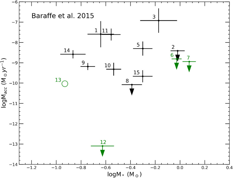
Figure 11. Plot of log(Macc) vs. log(M*) for our YSO sample, using masses derived from the I. Baraffe et al. (2015) evolutionary model. Class II YSOs are shown in black, and class III YSOs are shown in green. Objects are annotated with their indices according to Table 10. Upper limits on log(Macc) are denoted with downward arrows. Object 4 does not fall within the mass range of I. Baraffe et al. (2015) and is therefore not included in this plot. Object 13 is represented by a green open circle because its log(M*) and log(Macc) are approximate.
Download figure:
Standard image High-resolution image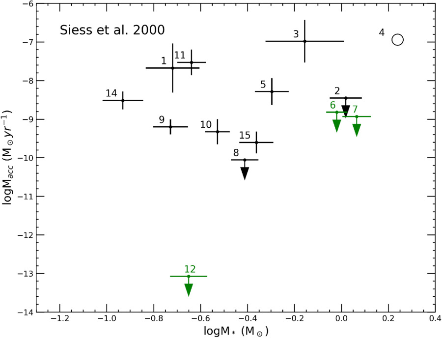
Figure 12. Plot of log(Macc) vs. log(M*) for our YSO sample, using masses derived from the L. Siess et al. (2000) evolutionary model. Plotting conventions are the same as in Figure 11. Object 13 does not fall within the mass range of L. Siess et al. (2000) and is not included in this plot. Object 4 is represented by a black open circle because its log(M*) and log(Macc) are approximate.
Download figure:
Standard image High-resolution imageThe extinction-corrected emission-line fluxes are converted into line luminosities using the distance to each YSO. We propagate uncertainty in distance by using the entire posterior distribution in distance of each target (described in Section 4.3.2) for each calculation. In Figures 13 and 14, the resulting line luminosities and uncertainties are plotted against the continuum-derived Lacc for our sample. The empirical relationship from J. M. Alcalá et al. (2017) for each line is then plotted as a dotted red line. It is important to note that each line is not fitted to our data; it is completely independently derived by J. M. Alcalá et al. (2017) but shows remarkable agreement with our data. If we apply the relationships from J. M. Alcalá et al. (2017) to each Lline of our sample, we then acquire another estimate for the accretion luminosity. We then take the average of the estimates from each emission line, deriving a new quantity we call Lacc,line. We calculated Lacc,line for every object except for the class III Objects 6 and 7, since almost all of their line fluxes are only upper limits. Ultimately, we find that applying the updated relationships from J. M. Alcalá et al. (2017) to the line luminosities of our class II sample yields Lacc,line in good agreement with each Lacc derived in Section 5.2. Figure 15 shows Lacc,line plotted against the continuum-derived Lacc. This plot visually demonstrates an approximate 1:1 correlation, suggesting trustworthiness of our new Bayesian approach. The only exception is the class III Object 12, which has Lacc,line = 0.36 and an upper limit on Lacc≤ −6.28 that lies well outside of the plot limits. This very likely nonaccretor has significant emission lines (unlike Objects 6 and 7), but the lines could possibly be attributed mainly to chromospheric activity.
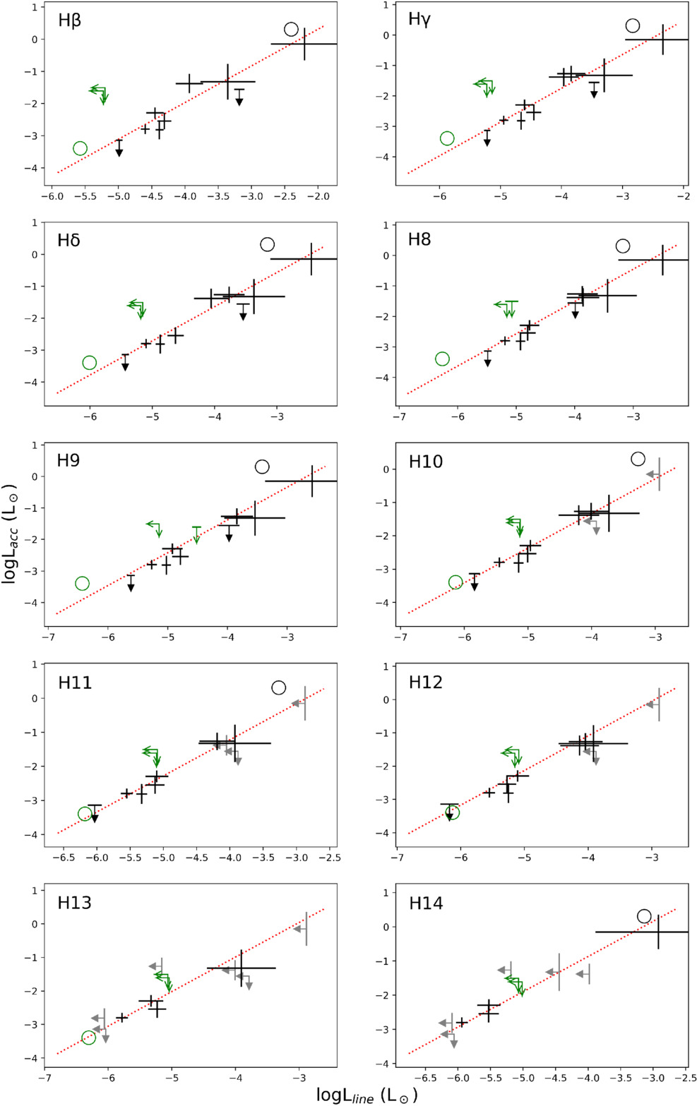
Figure 13. Continuum-derived accretion luminosity Lacc of both the class II and class III sample plotted against line luminosity for a variety of emission lines studied in J. M. Alcalá et al. (2017). Each emission line is labeled on the top left of the plot. For the class II YSOs, detected lines are plotted in black, and lines with only upper limits are plotted in gray. For class III YSOs, all results are plotted in green with empty arrows. Measurements for objects 4 and 13, which have only an approximate Lacc, are represented with circles. The red dotted line represents the relation from J. M. Alcalá et al. (2017), and is not a line fitted to our data.
Download figure:
Standard image High-resolution image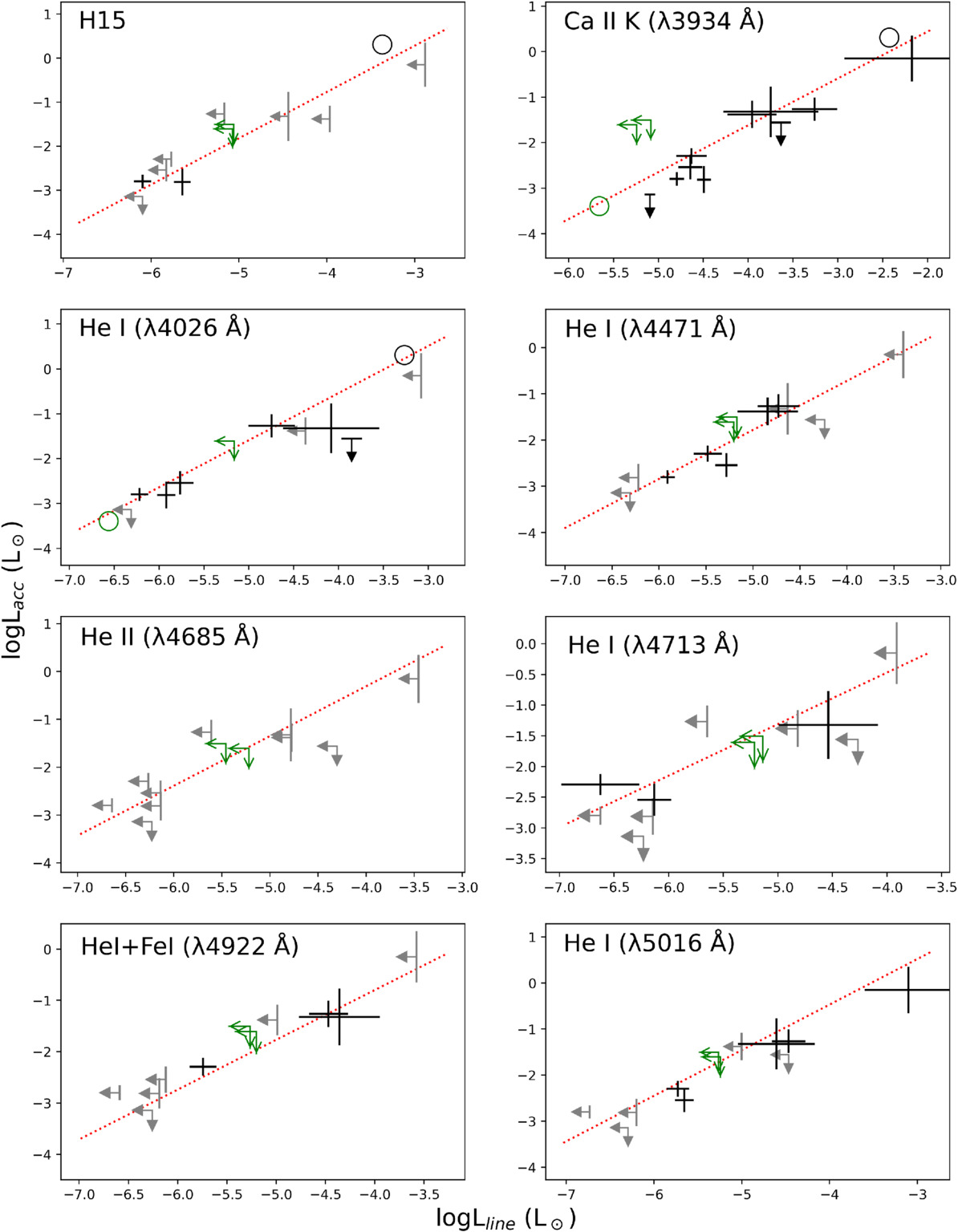
Figure 14. Continuum-derived accretion luminosity Lacc of both the class II and class III sample plotted against line luminosity for a variety of emission lines studied in J. M. Alcalá et al. (2017). The plot conventions are the same as Figure 13.
Download figure:
Standard image High-resolution image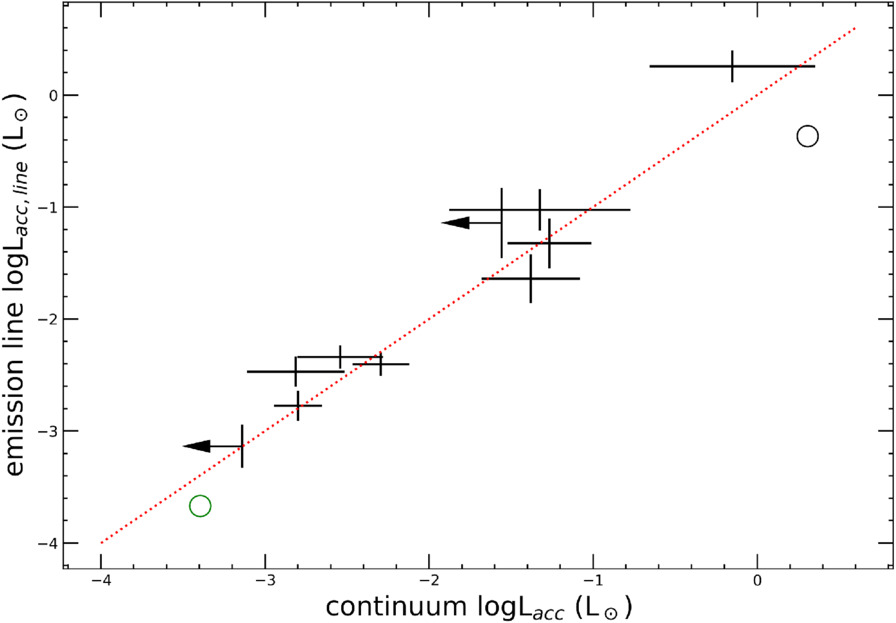
Figure 15. The average Lacc,line plotted against the continuum-derived Lacc for the class II stars (black) as well as Object 13, a class III star (green). Lacc,line is derived using emission-line luminosities and the relations from J. M. Alcalá et al. (2017). Objects 4 and 13, having only an approximate Lacc and Lacc,line, are represented with open circles. The red dotted line illustrates the approximate 1:1 correlation.
Download figure:
Standard image High-resolution imageEmission lines are produced by chromospheric activity in addition to accretion processes. This adds a bias to Lacc,line, which needs to be assessed. We check the Lacc,line of each star relative to L* to evaluate whether any of the YSOs in our current sample can be considered “weak accretors” having emission-line fluxes dominated by chromospheric activity. Figure 16 shows the ratio log(Lacc,line/L*) plotted against Teff for each object. The red dashed line shows the level at which chromospheric noise is expected to become important, as derived by C. F. Manara et al. (2013b) using a set of class III YSOs. The orange dashed line shows the update for 4000K < Teff < 5800K objects, made by C. F. Manara et al. (2017a). Finally, the blue dashed line shows the chromospheric noise level derived by R. A. B. Claes et al. (2024), with the Teff scale converted from G. J. Herczeg & L. A. Hillenbrand (2014) to the one used in this work (K. L. Luhman et al. 2003 for M-type stars, and S. J. Kenyon & L. Hartmann 1995 for K-type stars).
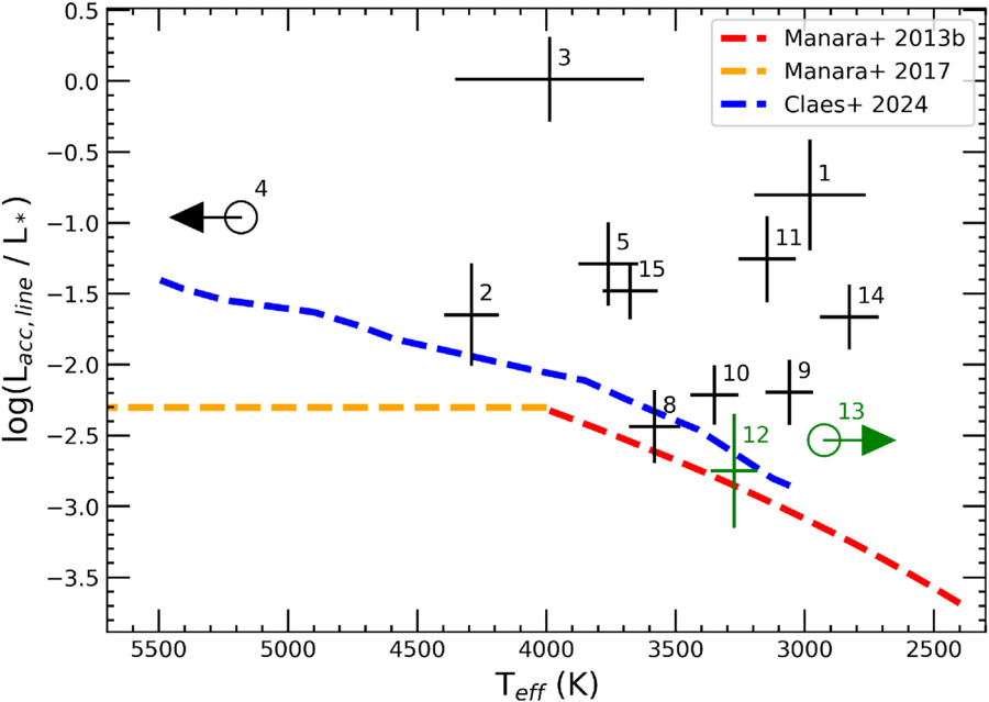
Figure 16. The ratio of the average Lacc,line with L* for each star for which Lacc,line had been measured. The ratio is plotted in a logarithmic scale against Teff. Class II YSOs are plotted in black, and the two class III YSOs are plotted in green. The red and orange dashed lines mark the approximate boundary below which chromospheric emission becomes an important contributor to Lacc, according to C. F. Manara et al. (2013b) and C. F. Manara et al. (2017a). The blue dashed line marks the same but according to R. A. B. Claes et al. (2024), with the Teff scale converted from G. J. Herczeg & L. A. Hillenbrand (2014) to the one used in this work in Section 4.1. Objects 4 and 13, having only an approximate Lacc,line, are represented with open circles.
Download figure:
Standard image High-resolution imageAmong the two class III YSOs for which Lacc,line was calculated, Object 12 is the closest to the chromospheric threshold of C. F. Manara et al. (2013b), and is below that of R. A. B. Claes et al. (2024). This implies that the log(Lacc,line) value for this object is overestimated due to chromospheric line emission. Indeed, the upper limit of log(Lacc) found by fitting to the continuum is lower than the log(Lacc,line) value by approximately 2.5 dex. The two class II YSOs with upper limits on the Lacc derived in the continuum fit (Objects 2 and 8) also both demonstrate emission-line fluxes at or near to the chromospheric level. In Figure 16, Object 8 has a log(Lacc,line/L*) that lies under the chromospheric threshold of R. A. B. Claes et al. (2024). Object 2 has a higher log(Lacc,line/L*) lying slightly above the threshold. These objects are both plausible “weak accretors” by separate consideration of both their continuum emission and their emission lines.
7. Discussion
7.1. Parameter Probabilities and Correlations
We have demonstrated an improved method to fitting an accretion model to YSO spectra by using a Bayesian framework. One main motivation in using a Bayesian approach is to understand hidden correlations among the parameters. From our small sample of YSOs, we have noticed several trends in behavior.
The quantity log(Lacc) often exhibits correlation with AV. Uncertainties in AV can therefore have a particularly strong influence on the determination of log(Lacc). The left-hand side of Figure 17 shows the overlaid posteriors of log(Lacc) versus AV for every object in the class II sample for which log(Lacc) is not an upper limit. Within individual posteriors, a strong correlation is often evident between AV and log(Lacc). Moreover, there is a scattered trend that the objects with a higher median log(Lacc) value tend to have the higher median AV values. This degeneracy between the intrinsic luminosity of the accretion slab and the extinction could be partially improved by analyzing YSO spectra with a wider wavelength coverage. C. F. Manara et al. (2013a) pointed out that if one fits the model to a broader wavelength range (such as that of X-Shooter) or even just includes more photometric data from other bands in addition to the spectroscopic data, the reddening effect of extinction and the blue enhancement by the accretion slab may be better disentangled, although never completely. We also find that Kphot and AV typically appear correlated. This makes sense, since Kphot and AV both pertain directly to the scaling of the class III photospheric template and can be adjusted somewhat interchangeably, resulting in degeneracy. This can introduce a degeneracy of log(L*) with AV as well, although we find that the correlation between these two is less pronounced, as shown in the right-hand side of Figure 17.
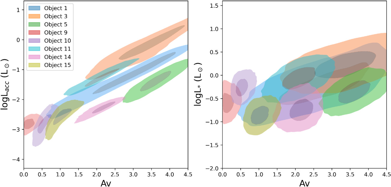
Figure 17. The overlaid posteriors for log(Lacc) and log(L*) vs. AV, for every object in our sample in which log(Lacc) is not an upper limit or is approximated. A strong correlation can be seen between AV and log(Lacc) in particular.
Download figure:
Standard image High-resolution imageExamining the corner plots in Appendix B, there is often a notable lack of correlation between log(Lacc) and the parameters that make up the slab portion of the model: Tslab, ne, and τ0. This is true both within individual posteriors and also over the entire sample; for example, objects with a high median Tslab value do not demonstrate higher or lower median Lacc values than other objects. As previously noted in E. Rigliaco et al. (2012), there are degeneracies in the slab model, in which trade-offs of different slab parameters are able to produce similar accretion luminosities. E. Rigliaco et al. (2012) found that reasonable slab model fits to a YSO spectrum yielded Lacc estimates within only ∼10% of each other, even over a wide variety of slab parameters. C. F. Manara (2014) included a full discussion of the interplay of these three parameters, and how they each affect the shape of the slab model. The Bayesian method shows us that these are nuisance parameters that can be marginalized over. Instead, only the overall scaling of the slab model Kslab tends to demonstrate some correlation with log(Lacc) in the corner plots, alongside the extinction AV.
Within our current sample, we find only one instance in which the model fit shows clear preference for a certain Tslab value between the upper and lower bounds: Object 13 has a Tslab posterior that peaks at ∼7000K with a symmetric distribution. In other cases, we mainly find broad probability distributions for Tslab that are either relatively flat or skewed to low temperatures. The least-constrained parameter tends to be ne. We find that ne often does not display a strong peak in probability at any one specific value between the imposed lower and upper bounds of 1010 cm−3 and 1016 cm−3. In most cases, the distribution for log(ne) gradually rises to peak probability at ∼10 or ∼16, or remains nearly flat. For τ0, we find only two instances where the model settles on a specific value between the lower and upper bounds of 0.01 and 5.0. These are Objects 11 and 14, for which the most probable τ0 is ∼3.5 and ∼4.0, respectively. We more often find τ0 skewed to the lowest or highest values possible, and otherwise a flat distribution or somewhat bimodal distribution between both extremes.
Interestingly, we notice that there is sometimes a correlation between Tslab and log(ne) for Tslab values below ∼10,000K. This can be seen most clearly in the corner plots for Objects 1, 5, 9, 10, 11, and 15. One possible reason for the correlation is the way that Tslab and ne jointly affect the height of the Balmer jump (i.e., the ratio of flux at 3600 Å and 4000 Å). C. F. Manara (2014) showed that a specific value for the Balmer jump can be achieved for higher and higher Tslab, as long as ne is also increased. However, the ratio gradually becomes independent of ne at high Tslab values. A similar phenomenon occurred when C. F. Manara (2014) examined the ratio of Balmer continuum emission to Paschen continuum emission.
Three of the lowest-mass class II stars (Objects 1, 11, and 14) demonstrate both high Tslab and τ0 values, and display an apparent anticorrelation between these two parameters for Tslab > 10,000 K. In their work, C. F. Manara (2014) showed how either increasing τ0 or increasing Tslab can suppress the strength of features such as the height of the Balmer jump and the slope of the Balmer continuum. This trade-off may be one possible reason for the anticorrelation. Such a phenomenon may be particularly noticeable for these three objects because the Balmer jump is a fairly dominant component in their spectra, and because their Tslab and τ0 posterior distributions happen to both prefer higher values.
C. F. Manara (2014) discussed the trustworthiness of the slab model for the sole purpose of determining Lacc. As we alluded to in Section 4.1, the slab model is based off an older paradigm for accreting YSOs, where particles cross a boundary layer between the inner circumstellar disk and the star (e.g., D. Lynden-Bell & J. E. Pringle 1974). This is different from the presently more widely accepted magnetospheric accretion model. Therefore, the three parameters Tslab, ne, and τ0 of the slab model should not be interpreted as physical quantities due to their lack of basis in reality. According to C. F. Manara (2014), however, there are a number of reasons why the slab model is still useful other than its simplicity. One reason is that more complex “shock models” based in magnetospheric accretion (e.g., that of N. Calvet & E. Gullbring 1998) have not been able to fully match the veiling of spectra for accreting class II stars at long wavelengths (L. Ingleby et al. 2013). However, the slab model has been able to match observations (e.g., J. A. Valenti et al. 1993; G. J. Herczeg & L. A. Hillenbrand 2008). Moreover, for smaller wavelengths of ≲3000 Å, using either model has yielded similar bolometric correction factors for the accretion luminosity Lacc (e.g., N. Calvet & E. Gullbring 1998; G. J. Herczeg & L. A. Hillenbrand 2008; C. F. Manara 2014). Therefore, the slab model, which is simple to implement with only a few parameters, is often still used. Nonetheless, it is sensible to treat the model with some caution given its dubious physical origins. Continued tests on YSO spectra at a variety of photometric wave bands can further verify the usefulness of the slab model for calculating Lacc.
7.2. Comparison to Specific SFRs
We have studied only a small sample of YSOs that do not all belong to one star-forming region. We therefore refrain from making physical interpretations of our results for Macc. Instead, our study offers a prototype of what can be accomplished with optical/UVB spectroscopy of YSOs, combined with our Bayesian framework for fitting the accretion model, which can be applied to larger surveys in the future. With our small sample, we can at least note that our results for the L*–Lacc plot (Figure 8) and M*–Macc plots (Figures 11 and 12) occupy a similar range as in previous studies of various star-forming regions. We briefly compare to previous results of class II stars from Lupus (J. M. Alcalá et al. 2017), Chamaeleon I (C. F. Manara et al. 2016), and NGC 1333 (E. Fiorellino et al. 2021).
Figure 18 shows that the L* and Lacc of our class II sample follow a loose linear relationship in agreement with these three star-forming regions. A few objects in our current sample (Objects, 8, 9, and 10) have fairly low Lacc/L* compared to most objects, but they are still certainly plausible, as several stars from Lupus and Chamaeleon I demonstrate similarly low Lacc/L* values or upper limits.
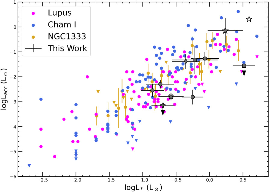
Figure 18. Plot of the continuum-derived log(Lacc) vs. log(L*) for the class II targets of our sample, compared to the results for class II YSOs from Lupus (J. M. Alcalá et al. 2017), Chamaeleon I (C. F. Manara et al. 2016), and NGC 1333 (E. Fiorellino et al. 2021). These three sets are plotted in magenta, blue, and orange, respectively, with upper limits represented by triangles. The values from this work are plotted in black and gray, with different shapes for different regions: circles (NGC 1333), stars (NGC 7000), squares (IC 5146), a diamond (Serpens), a plus sign (Orion), and an X-symbol (Perseus). Object 4, having only an approximate Lacc, is represented with an unfilled star.
Download figure:
Standard image High-resolution imageFigure 20 shows how the M*–Macc relationship from our current sample of 15 YSOs compares to Lupus, Chamaeleon I, and NGC1333. Past studies have demonstrated a loose correlation between M* and Macc. Given our small sample size, we do not attempt to fit a line to log(M*)–log(Macc) plot. However, we note that our sample, although scattered, occupies a space similar to these three star-forming regions. The highest accretion rates in our current sample are attained by objects 3 and 4 (respectively, log(Macc) = −6.99 and log(Macc) ≈ −6.93 in M⊙ yr−1; via the L. Siess et al. 2000 evolutionary model). Although high, these accretion rates are similar to several objects from Chamaeleon I. We also observe a relatively high Macc/M* ratio for objects 1, 11, and 14. Although they lie along the high-Macc border of the M*–Macc relationships for Lupus, Chamaeleon I, and NGC 1333, they are not implausibly high. Objects 1 and 11 are both from NGC 1333 and are within expectations when compared to similar-mass class II YSOs studied by E. Fiorellino et al. (2021).
There are two class II YSOs in the sample for which we derive only upper limits on mass accretion rate. Object 8 (CVSO 1897) demonstrates the lowest mass accretion rate among all of the class II stars, with an upper limit of log(Macc) ≤–10.0 in M⊙ yr−1. This upper limit lies along the low-Macc border of the M*–Macc plots found for Lupus, Chamaeleon I, and NGC 1333. As can be seen in Figure 19, Object 8 has a lower accretion rate than Object 10 (EM* LkHA 351), even though Object 10 has a lower spectral index α (being nearly in the class III category). Though Object 8 has a class II SED, its spectrum appears similar to a class III star. As shown in Figure 16 and previously discussed in Section 6, Object 8 has emission-line fluxes close to the expected chromospheric level for its Teff, according to the thresholds defined by C. F. Manara et al. (2013b) and R. A. B. Claes et al. (2024). One other measurement for the accretion rate of Object 8 has been made by E. Manzo-Martìnez et al. (2020), and they found a log(Macc) of −9.12 in M⊙ yr−1. They derived this accretion rate using the equivalent width of the Hα emission line. While their estimated Macc is above ours, their estimates for AV, L* and M* are similar. They found an AV = 0.14 mag, log(L*/L⊙) = −0.80, and log(M*/M⊙) = −0.48, while we derive an AV = 0.12 ± 0.09 mag, log(L*/L⊙) = −0.70 ± 0.17, and log(M*/M⊙) = −0.41 ± 0.06 using the L. Siess et al. (2000) models. The other upper limit in Macc within our sample is Object 2, one of the highest-mass stars in the sample with M* ≈ M⊙. Object 2 demonstrates an upper limit of log(Macc) ≤ −8.4. Similarly to Object 8, Object 2 also has emission-line fluxes close to the expected chromospheric level in Figure 16.
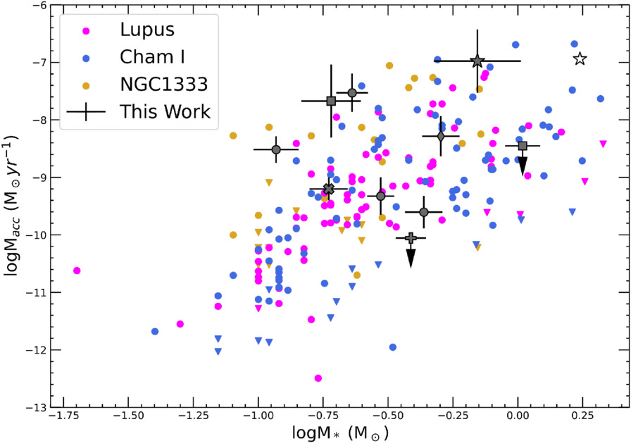
Figure 19. Plot of log(Macc) vs. log(M*) for the class II targets of our current sample, compared to the results for class II YSOs from Lupus (J. M. Alcalá et al. 2017), Chamaeleon I (C. F. Manara et al. 2016), and NGC1333 (E. Fiorellino et al. 2021). These three sets are plotted in magenta, blue, and orange, respectively, with upper limits represented by triangles. The values from this work are plotted in black and gray, with different shapes for different regions: circles (NGC 1333), stars (NGC 7000), squares (IC 5146), a diamond (Serpens), a plus sign (Orion), and an X-symbol (Perseus). Object 4 in NGC 7000, having only an approximate Macc, is represented with an unfilled star.
Download figure:
Standard image High-resolution image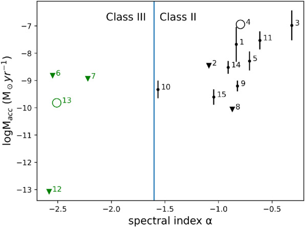
Figure 20. Plot of log(Macc) vs. the spectral index α used for YSO classification in Section 3. Class II YSOs are plotted in black, and Class III YSOs are plotted in green. Upper limits in Macc are denoted by downward triangles. Objects 4 and 13, having only an approximate Macc, are represented with open circles. The blue line is the dividing line between Class II and Class III in T. P. Greene et al. (1994).
Download figure:
Standard image High-resolution imageThere is one other star in our sample, Object 14 (2MASS J03284782+3116552), for which we found a mass accretion rate measurement in previous literature. This object is present in the E. Fiorellino et al. (2021) study of NGC1333. E. Fiorellino et al. (2021) found that the star has log(L*/L⊙) = −0.72, in agreement our result of log(L*/L⊙) = −0.74 ± 0.2. Using the fluxes of the Paβ and Brγ lines and applying the empirical line luminosity relations from J. M. Alcalá et al. (2017), they found log(Lacc/L⊙) = −1.95 ± 0.36. This is larger than the log(Lacc/L⊙) = −2.30 ± 0.18 found in our study. Using the L. Siess et al. (2000) models, we estimate M* = 0.12M⊙, in close agreement to the M* = 0.11M⊙ mass from E. Fiorellino et al. (2021). However, we find a lower accretion rate of log(Macc) = −8.81 ± 0.25 in M⊙ yr−1, as opposed to their log(Macc) = −8.13. The disagreement could potentially be ascribed to the difference in AV estimated. E. Fiorellino et al. (2021) estimated AV = 4.0 mag by fitting the J and H bands of the class II spectrum with a class III template by hand. We estimate AV = 2.1 though, using a similar process but in the near-UV and optical range. The disagreement may also be due to the underlying chromospheric activity, or differences in the choice of photospheric template between our work and E. Fiorellino et al. (2021). Besides Objects 8 and 14, there were no other literature values to compare with our sample, as far as we are aware.
The scatter in the log(M*)−log(Macc) relationship for previous works suggests that Macc depends on more than just M*. The aformentioned studies of Lupus, Chamaeleon I, and NGC 1333 each used samples of YSOs from single star-forming regions and, therefore, were all borne from the same local conditions at roughly the same time (although possibly with some spread in age; see the discussion in C. F. Manara et al. 2023 regarding age gradients within regions). As a result, scatter in the log(M*)–log(Macc) found by these studies can be more confidently attributed to individual differences in disk mass or the angular momentum of prenatal cores, or perhaps to time variability in accretion. On the other hand, the YSOs of our current sample have the additional complication of being from several SFRs rather than just one. Within singular star-forming regions, we do still note this definite diversity in Macc. A prime example is the difference in Macc between Objects 9 and 11. Both of these class II YSOs belong to NGC 1333 and have nearly the same mass (0.23 M⊙ and 0.19 M⊙, respectively; via L. Siess et al. 2000 models). However, they display Macc that differ by ≈1.5 dex. Object 11, the stronger accretor, has a spectrum that displays a visibly much more dramatic Balmer jump compared to Object 9.
8. Conclusion
We have developed a Python-based package called nuts-for-ysos and used it to study the spectra of 15 photometrically identified YSOs from VIRUS parallel data. With a wavelength range of 3500–5500 Å, VIRUS captures several important accretion indicators in YSOs, including the excess Balmer continuum and a variety of optical emission lines. Within nuts-for-ysos, we applied the No U-Turn Sampler (NUTS) to fit a model consisting of a theoretical accretion spectrum added to a class III YSO template, in order to replicate the continuum of our 15 VIRUS spectra. In doing so, we were able to simultaneously derive values for several stellar parameters and accretion parameters while examining uncertainties and covariances to an extent not achieved in the past. From these parameters, we were then able to determine mass accretion rates for each YSO. One main takeaway is the strong correlation between AV and Lacc derived from the model fits. This highlights the importance of precisely determining AV in order to constrain Lacc. This can better be achieved by fitting the model over a wide wavelength range, to differentiate the effects of extinction and accretion on the spectrum as much as possible. We then compared our results to those acquired using emission lines of the spectra, and found strong agreement. In comparing our study to previous studies of Lupus, Chamaeleon I, and NGC 1333, we also found our results to occupy a typical range in Lacc and Macc.
Our results demonstrate the promise of applying a Bayesian framework like nuts-for-ysos for analyzing YSO spectra. The nuts-for-ysos code is flexible with regards to the number and types of spectral features it fits for, as well as the wavelengths of these features. It can therefore be applied to both future VIRUS observations or to observations from other spectrographs. Regardless, a future cohesive analysis of a larger collection of YSOs will be especially important for better characterizing the relationship between M* and Macc. This, in turn, could help elucidate the physics behind star formation and by association the formation of planets.
Acknowledgments
We thank the anonymous referee for providing insightful comments that informed edits to our manuscript. Observations were obtained with the Hobby-Eberly Telescope (HET), which is a joint project of the University of Texas at Austin, the Pennsylvania State University, Ludwig-Maximilians-Universität München, and Georg-August-Universität Göttingen. The HET is named in honor of its principal benefactors, William P. Hobby and Robert E. Eberly.
VIRUS is a joint project of the University of Texas at Austin, Leibniz-Institut für Astrophysik Potsdam (AIP), Texas A&M University (TAMU), Max-Planck-Institut für Extraterrestrische Physik (MPE), Ludwig-Maximilians-Universität Muenchen, Pennsylvania State University, Institut für Astrophysik Göttingen, University of Oxford, and the Max-Planck-Institut für Astrophysik (MPA). In addition to Institutional support, VIRUS was partially funded by the National Science Foundation, the State of Texas, and generous support from private individuals and foundations.
The authors acknowledge the Texas Advanced Computing Center (TACC) at The University of Texas at Austin for providing high-performance computing, visualization, and storage resources that have contributed to the research results reported within this paper.
Computations for this research were performed on the Pennsylvania State University’s Institute for Computational and Data Sciences’ Roar supercomputer. The Center for Exoplanets and Habitable Worlds is supported by the Pennsylvania State University and the Eberly College of Science.
This work has made use of data from the European Space Agency (ESA) mission Gaia (https://www.cosmos.esa.int/gaia), processed by the Gaia Data Processing and Analysis Consortium (DPAC, https://www.cosmos.esa.int/web/gaia/dpac/consortium). Funding for the DPAC has been provided by national institutions, in particular the institutions participating in the Gaia Multilateral Agreement.
This publication makes use of data products from the Wide-field Infrared Survey Explorer, which is a joint project of the University of California, Los Angeles, and the Jet Propulsion Laboratory/California Institute of Technology, funded by the National Aeronautics and Space Administration.
The Pan-STARRS1 Surveys (PS1) and the PS1 public science archive have been made possible through contributions by the Institute for Astronomy, the University of Hawaii, the Pan-STARRS Project Office, the Max-Planck Society and its participating institutes, the Max Planck Institute for Astronomy, Heidelberg and the Max Planck Institute for Extraterrestrial Physics, Garching, The Johns Hopkins University, Durham University, the University of Edinburgh, the Queen’s University Belfast, the Harvard-Smithsonian Center for Astrophysics, the Las Cumbres Observatory Global Telescope Network Incorporated, the National Central University of Taiwan, the Space Telescope Science Institute, the National Aeronautics and Space Administration under grant No. NNX08AR22G issued through the Planetary Science Division of the NASA Science Mission Directorate, the National Science Foundation grant No. AST-1238877, the University of Maryland, Eotvos Lorand University (ELTE), the Los Alamos National Laboratory, and the Gordon and Betty Moore Foundation.
This work is based in part on observations made with the Spitzer Space Telescope, which was operated by the Jet Propulsion Laboratory, California Institute of Technology under a contract with NASA.
This research has made use of the VizieR catalog access tool, CDS, Strasbourg, France (DOI: 10.26093/cds/vizier). The original description of the VizieR service was published in F. Ochsenbein et al. (2000). This research has also made use of the SIMBAD database, operated at CDS, Strasbourg, France.
We also thank the Pennsylvania State University Erickson Discovery Grant for providing support to this project during Summer 2021. Funding from this grant paved the path to complete a portion of the analysis.
Software: PyMC (J. Salvatier et al. 2016), PyTensor (PyMC Team 2023; R. Al-Rfou et al. 2016), Matplotlib (J. D. Hunter 2007), NumPy (C. R. Harris et al. 2020), SciPy (P. Virtanen et al. 2020), Astropy (Astropy Collaboration et al. 2013, 2018, 2022), Specutils (Astropy-Specutils Development Team 2019), PySpecKit (A. Ginsburg & J. Mirocha 2011).
Appendix A: Data Reduction
The parallel observations were reduced using Remedy, a data processing pipeline for VIRUS.16
Remedy is responsible for calibrating the spectra from each individual fiber, and then combining these spectra into final “extracted spectra” of bright continuum sources. A full description of parallel observation reductions is presented in G. R. Zeimann et al. (2024), but we present relevant details to our study below. For each observation, Remedy first performs the gain multiplication, bias and dark frame subtractions, and masking of hot pixels identified in the master dark frame. The locations of the fibers on the detector are then determined using a master twilight frame compiled over several days. Wavelength calibration for each fiber is performed using Cd and Hg arc lamps. In order to extract complete spectra of continuum sources from the fiber spectra, a fiber normalization must be performed, which accounts for variations in CCD quantum efficiency and both fiber and spectrograph throughput variations. A master twilight frame is used to evaluate the relative throughput between each fiber and their average, and the fibers are normalized appropriately. A fiber is omitted from the extracted spectrum if its normalization factor is below 10%. For each exposure, a single sky model is constructed using identified “blank” fibers in the field. This first sky model is individually subtracted from every normalized fiber spectrum. Then a more localized residual sky model is subtracted, employing a Gaussian kernel in the fiber and wavelength direction. This kernel has a standard deviation of seven fibers in the fiber direction and 14 Å in the wavelength direction. Fibers with continuum emission >2σ are masked in this residual sky process. This entire sky subtraction process tends to fail in crowded fields with a lack of fibers pointed on blank sky. For example, several VIRUS parallel observations contained YSOs in nebulous regions such as the Orion Nebula. These observations were omitted from our study because the sky subtraction was unreliable. After sky subtraction, the VIRUS observations are then astrometrically calibrated using Pan-STARRS (Chambers & Pan-STARRS Team 2017) Data Release 2. Remedy matches point sources from each exposure with Pan-STARRS, and then shifts and rotates the VIRUS astrometry accordingly; shifts are usually <5” and rotations ≲0 1.
1.
Remedy then extracts continuum sources from the normalized, sky-subtracted, and astrometrically calibrated fiber spectra. The seeing at the HET is usually around the same as the 1 5 diameter of the VIRUS fibers, meaning that the weight for each fiber in receiving light from a source can easily change with the presumed position of the source. Another complication is the presence of differential atmospheric refraction, which causes variation in the throughput with wavelength for a given fiber. Both of these phenomena are especially problematic for parallel VIRUS observations, which are not dithered, and therefore sparsely sample the sky compared to the usual 3-point dither pattern of VIRUS observations. Remedy uses the other stars in the VIRUS FOV (usually more than 20) to model the spatial point-spread function (PSF) and the differential atmospheric refraction, so that it can address these issues and accurately extract the spectrum of the source.
Table 10. Observation Log
| ID | SIMBAD Name | Obs. date | R.A. | Decl. | Exp. time | Avg. SNR | PanSTARRS ID |
|---|---|---|---|---|---|---|---|
| 1 | 2MASS J21523325+4710505 | 2020-11-05 | 21:52:33.24 | 47:10:50.50 | 907.03 | 5.6 | 164613281385307509 |
| 2 | 2MASS J21533310+4716092 | 2020-11-05 | 21:53:33.10 | 47:16:09.20 | 907.03 | 52.1 | 164723283879153751 |
| 3 | 2MASS J20580138+4345201 | 2020-10-04 | 20:58:01.38 | 43:45:20.15 | 607.8 | 5.84 | 160503145057527374 |
| 4 | EM* LkHA 188 | 2020-12-01 | 20:58:23.81 | 43:53:11.40 | 608.15 | 138.56 | 160663145991974465 |
| 5 | 2MASS J18300610+0106170 | 2020-04-15 | 18:30:06.11 | 01:06:16.81 | 1207.45 | 10.93 | 109322775254456070 |
| 6 | 2MASS J18295618+0110574 | 2020-04-19 | 18:29:56.18 | 01:10:57.32 | 1207.8 | 58.24 | 109412774841009544 |
| 7 | V* V776 Ori | 2020-02-07 | 05:34:50.97 | −05:42:21.44 | 608.13 | 201.04 | 101150837123603275 |
| 8 | CVSO 1897 | 2020-11-15 | 05:40:15.14 | 00:57:26.71 | 1826.3 | 67.41 | 106850850630851552 |
| 9 | [HL2013] 052.17673+30.49810 | 2021-01-16 | 03:28:42.44 | 30:29:53.03 | 1506.9 | 53.16 | 144590521768208302 |
| 10 | EM* LkHA 351 | 2019-01-01 | 03:28:46.20 | 31:16:38.44 | 908.15 | 88.41 | 145530521924233432 |
| 11 | 2MASS J03285101+3118184 | 2019-01-01 | 03:28:51.03 | 31:18:18.39 | 908.15 | 47.75 | 145560522125686781 |
| 12 | 2MASS J03283651+3119289 | 2019-01-01 | 03:28:36.53 | 31:19:28.81 | 908.15 | 31.91 | 145590521521560240 |
| 13 | 2MASS J03292815+3116285 | 2021-02-09 | 03:29:28.16 | 31:16:28.44 | 1508.32 | 6.54 | 145530523673090085 |
| 14 | 2MASS J03284782+3116552 | 2021-02-09 | 03:28:47.84 | 31:16:55.05 | 1508.32 | 16.81 | 145530521992468976 |
| 15 | 2MASS J03285216+3122453 | 2021-02-09 | 03:28:52.17 | 31:22:45.15 | 1508.32 | 44.76 | 145650522173355698 |
| 16 | ATO J052.3580+31.4444 | 2021-02-12 | 03:29:25.93 | 31:26:39.93 | 1507.25 | 61.23 | 145730523580053950 |
Download table as: ASCIITypeset image
Each VIRUS parallel observation can ultimately contain hundreds to thousands of extracted spectra. Flux calibration is first performed on the extracted spectra using the throughput curve for the HETDEX collaboration (K. Gebhardt et al. 2012). Then, these preliminary calibrated spectra are convolved with the Pan-STARRS g filter. For each entire parallel observation, the overall biweight-estimated offset between the Pan-STARRS1 DR2 g magnitudes and VIRUS g magnitudes is then used to normalize this preliminary calibration. The finished flux calibration has a standard deviation of usually 0.1–0.15 mag. In this study, however, we chose to individually re-normalize extracted spectra using their Pan-STARRS1 DR2 “Mean PSF” g magnitudes (Chambers & Pan-STARRS Team 2017).17 This was because stars in star-forming regions may be young and variable in brightness, and these variations can affect a normalization done over an entire shot at once. Normalizing using photometry one at a time does not remove the possibility of each target’s variability affecting flux calibration, but it does allow for a more consistent approach not affected by the number and variability of neighboring stars. Moreover, we use the Pan-STARRS1 DR2 Mean PSF r and i magnitudes when fitting the accretion model to the VIRUS spectra in Section 4, so it is best that the g magnitudes of the VIRUS spectra are kept completely consistent with Pan-STARRS photometry. We are therefore assuming that the YSO spectrum has not drastically changed between the Pan-STARRS photometric observation and VIRUS observation. While this might be an unsuitable assumption for sources significantly varying in luminosity, like erupting FUors or EXors stars, none of our targets have previously been identified with these categories. The uncertainty in the Pan-STARRS photometry is taken into account when calculating the final uncertainty for each VIRUS spectrum. Table 10 lists the details of the VIRUS parallel observation corresponding to each object, as well as the name of the object in the SIMBAD database, the average SNR of the extracted spectrum, and the Pan-STARRS ID for each object.
Appendix B: Model Fit and Corner Plots
Included in Figures 21–50 are plots of the median model fit for each object, and the probability distributions for each model parameter. Moreover, for each object there are corner plots of the model parameters and of log(L*) and log(Lacc).
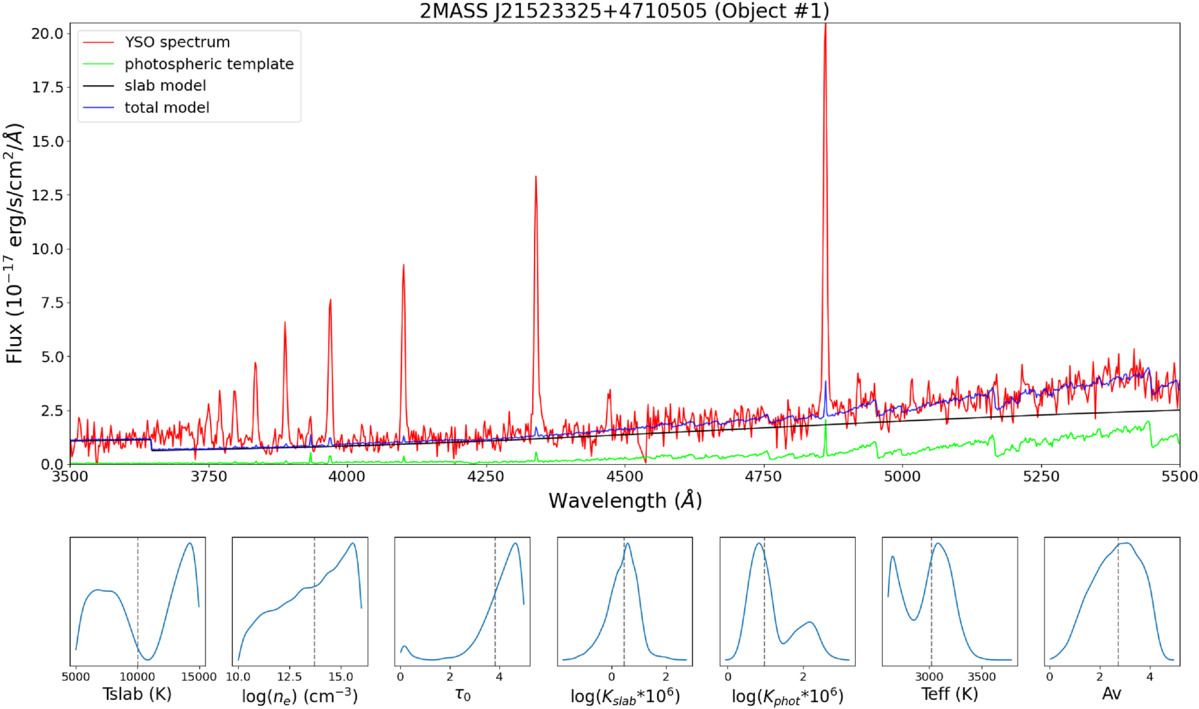
Figure 21. The median model fit for Object 1 and the parameter posteriors below (the median parameters marked with a vertical gray dotted line).
Download figure:
Standard image High-resolution image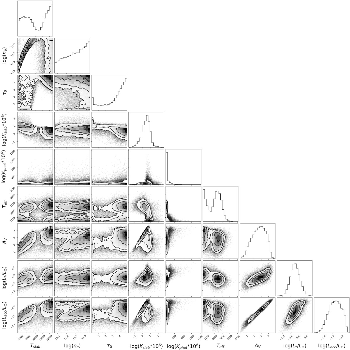
Figure 22. The corner plot for Object 1, for model parameters and the log(L*) and log(Lacc) posteriors.
Download figure:
Standard image High-resolution image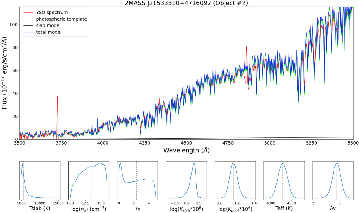
Figure 23. The median model fit for Object 2 and the parameter posteriors with the same plotting convention as Figure 21.
Download figure:
Standard image High-resolution image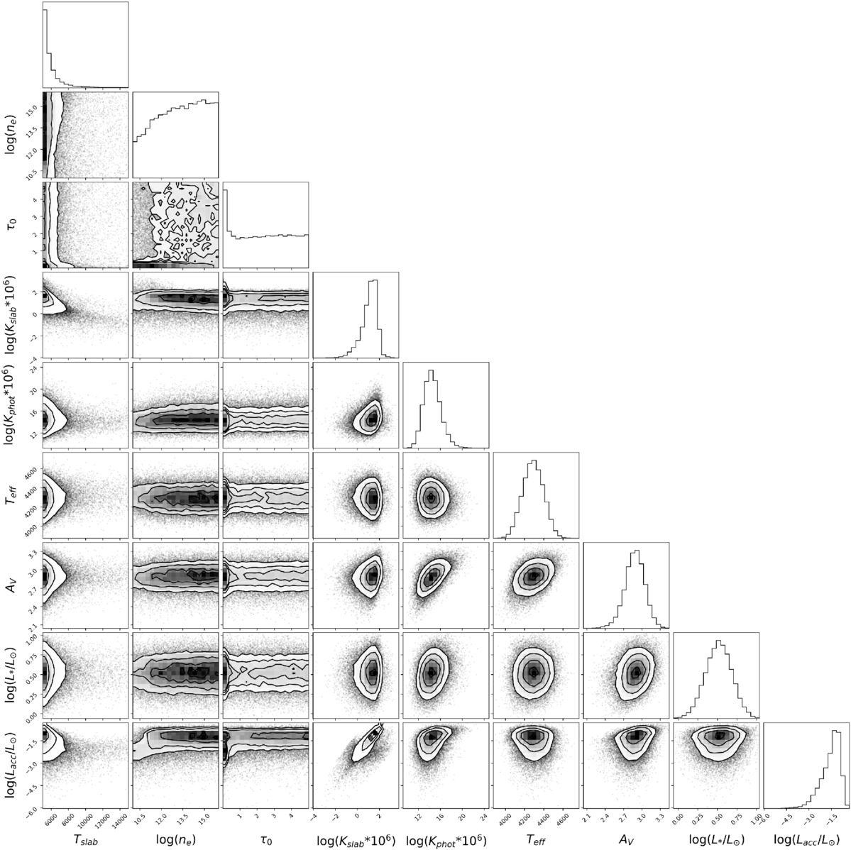
Figure 24. The corner plot for Object 2, for model parameters and the log(L*) and log(Lacc) posteriors.
Download figure:
Standard image High-resolution image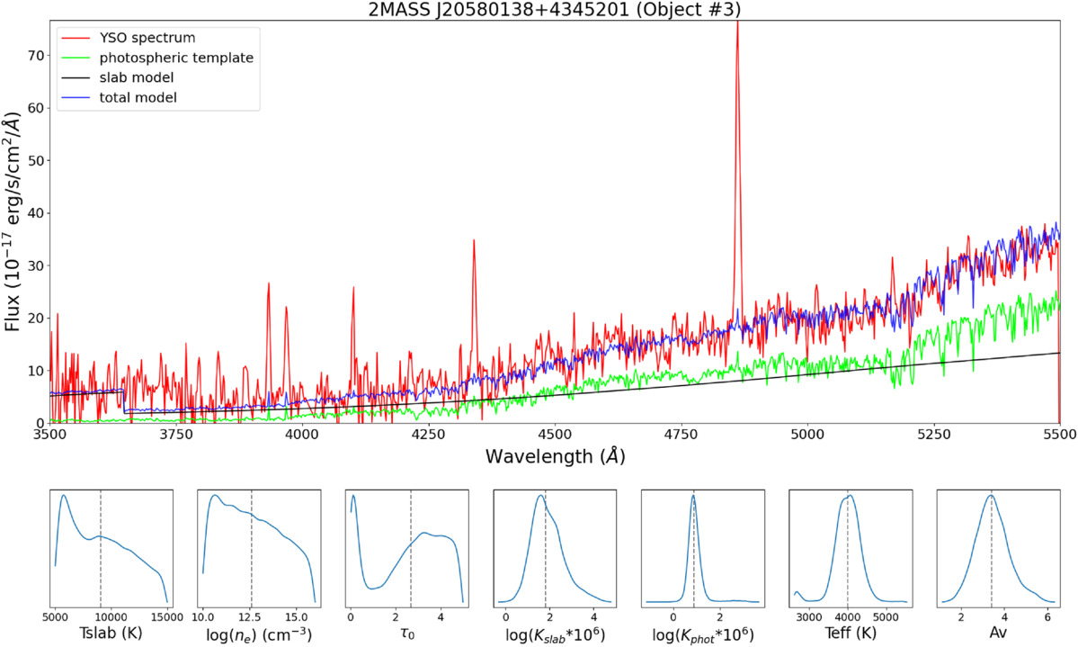
Figure 25. The median model fit for Object 3 and the parameter posteriors with the same plotting convention as Figure 21.
Download figure:
Standard image High-resolution image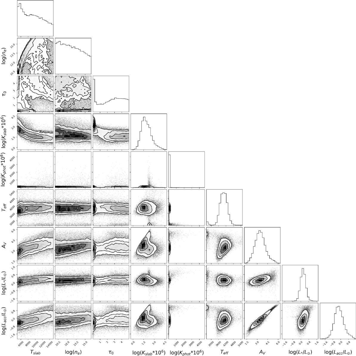
Figure 26. The corner plot for Object 3, for model parameters and the log(L*) and log(Lacc) posteriors.
Download figure:
Standard image High-resolution image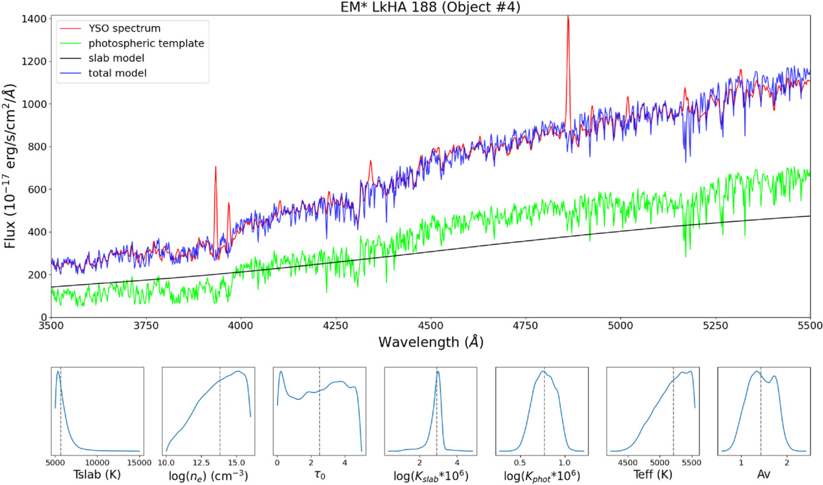
Figure 27. The median model fit for Object 4 and the parameter posteriors with the same plotting convention as Figure 21.
Download figure:
Standard image High-resolution image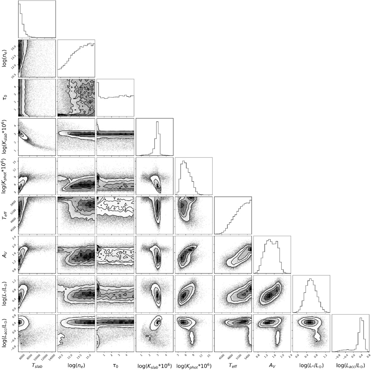
Figure 28. The corner plot for Object 4, for model parameters and the log(L*) and log(Lacc) posteriors.
Download figure:
Standard image High-resolution image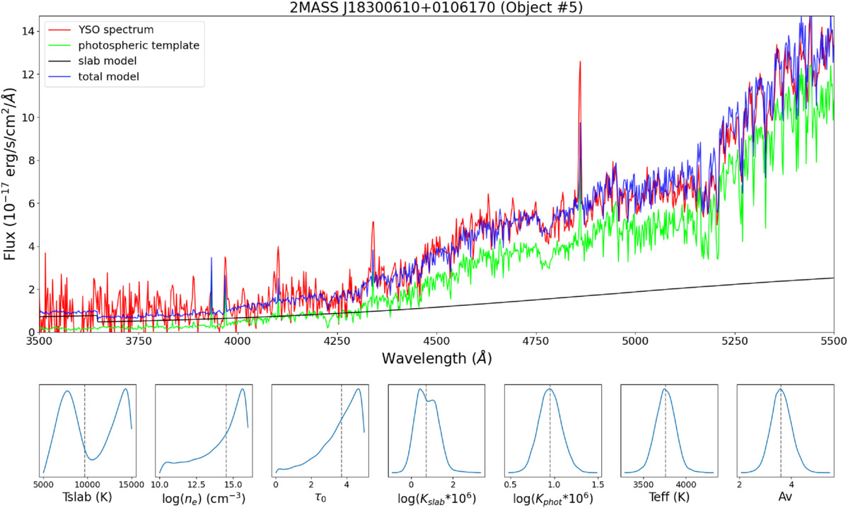
Figure 29. The median model fit for Object 5 and the parameter posteriors with the same plotting convention as Figure 21.
Download figure:
Standard image High-resolution image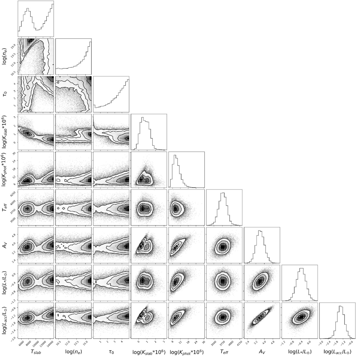
Figure 30. The corner plot for Object 5, for model parameters and the log(L*) and log(Lacc) posteriors.
Download figure:
Standard image High-resolution image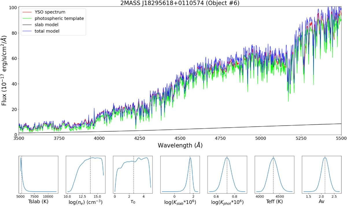
Figure 31. The median model fit for Object 6 and the parameter posteriors with the same plotting convention as Figure 21.
Download figure:
Standard image High-resolution image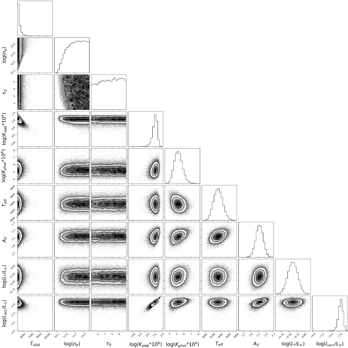
Figure 32. The corner plot for Object 6, for model parameters and the log(L*) and log(Lacc) posteriors.
Download figure:
Standard image High-resolution image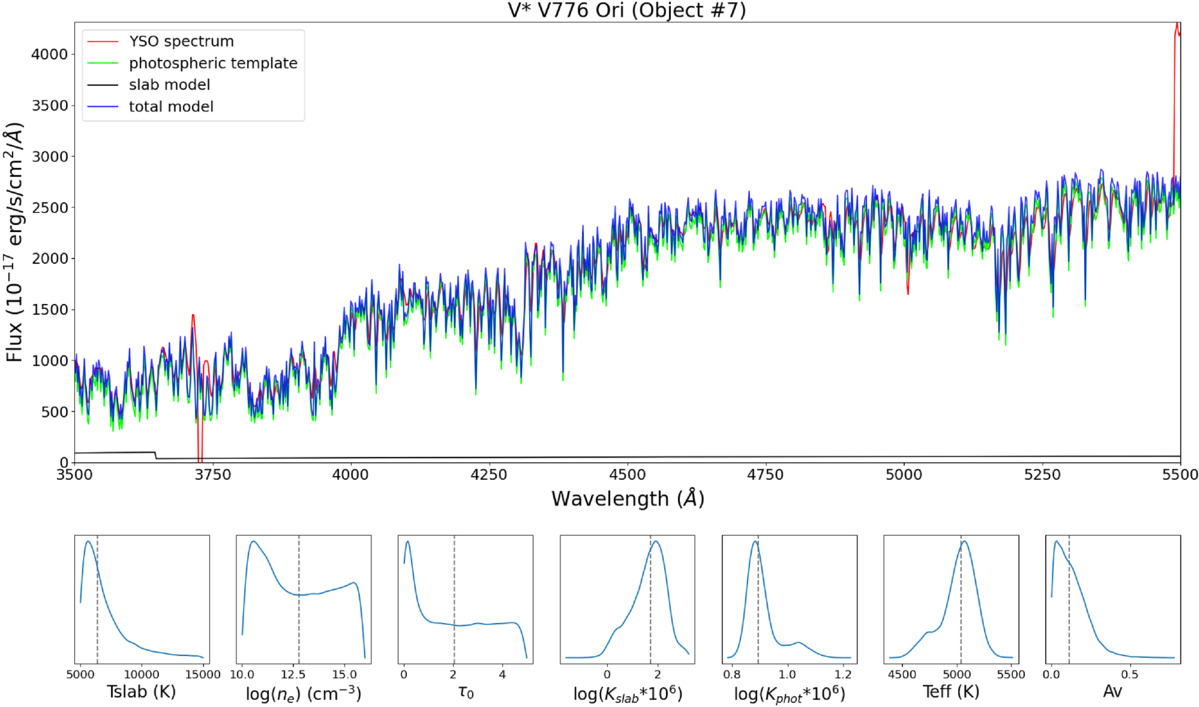
Figure 33. The median model fit for Object 7 and the parameter posteriors with the same plotting convention as Figure 21.
Download figure:
Standard image High-resolution image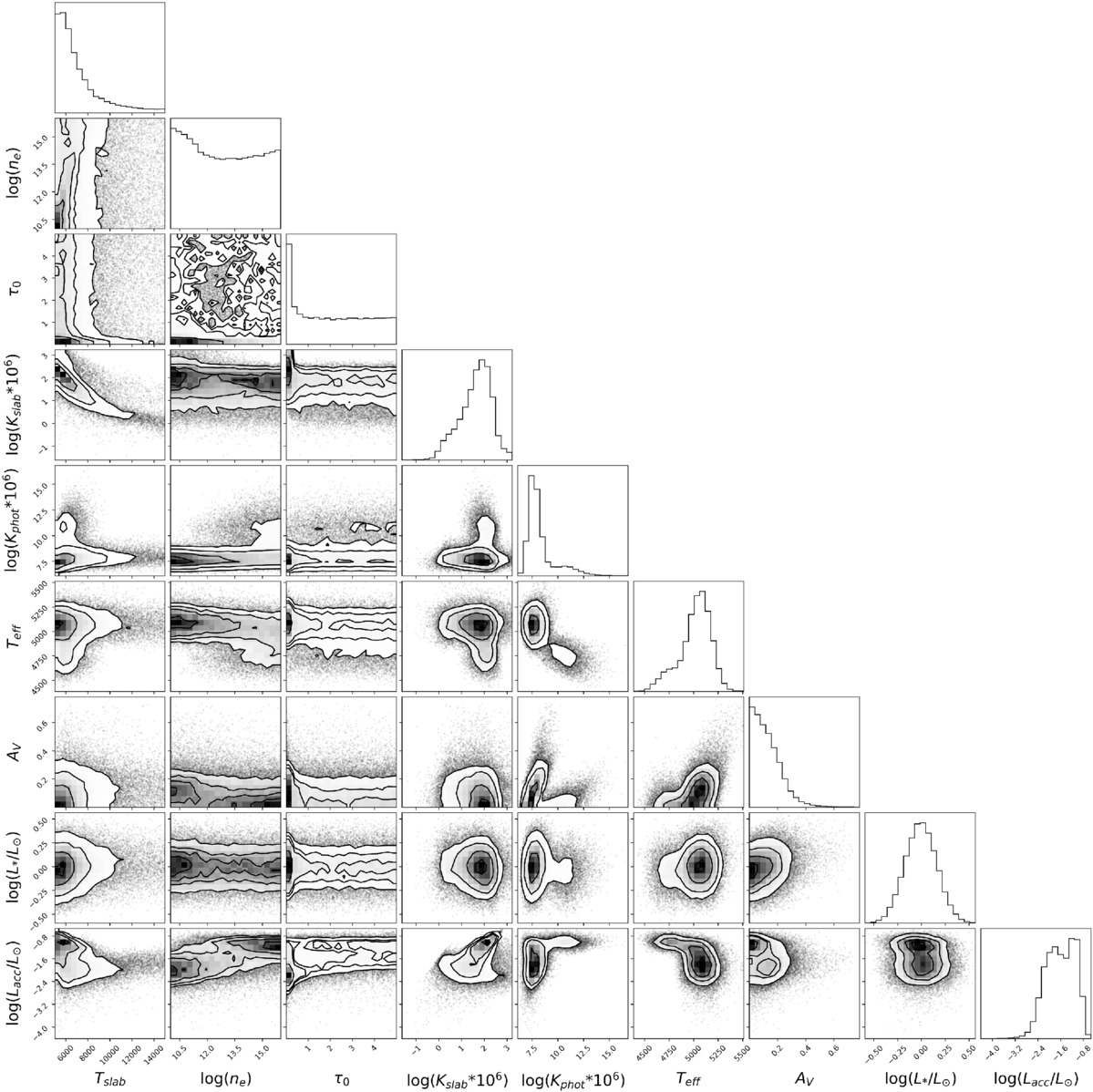
Figure 34. The corner plot for Object 7, for model parameters and the log(L*) and log(Lacc) posteriors.
Download figure:
Standard image High-resolution image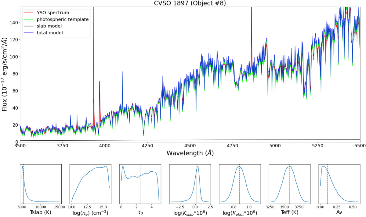
Figure 35. The median model fit for Object 8 and the parameter posteriors with the same plotting convention as Figure 21.
Download figure:
Standard image High-resolution image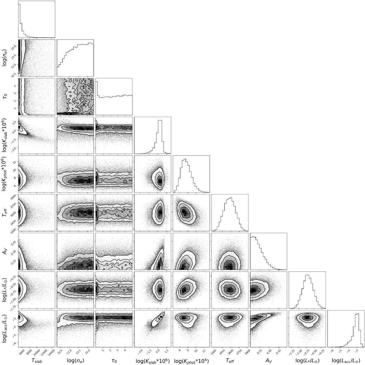
Figure 36. The corner plot for Object 8, for model parameters and the log(L*) and log(Lacc) posteriors.
Download figure:
Standard image High-resolution image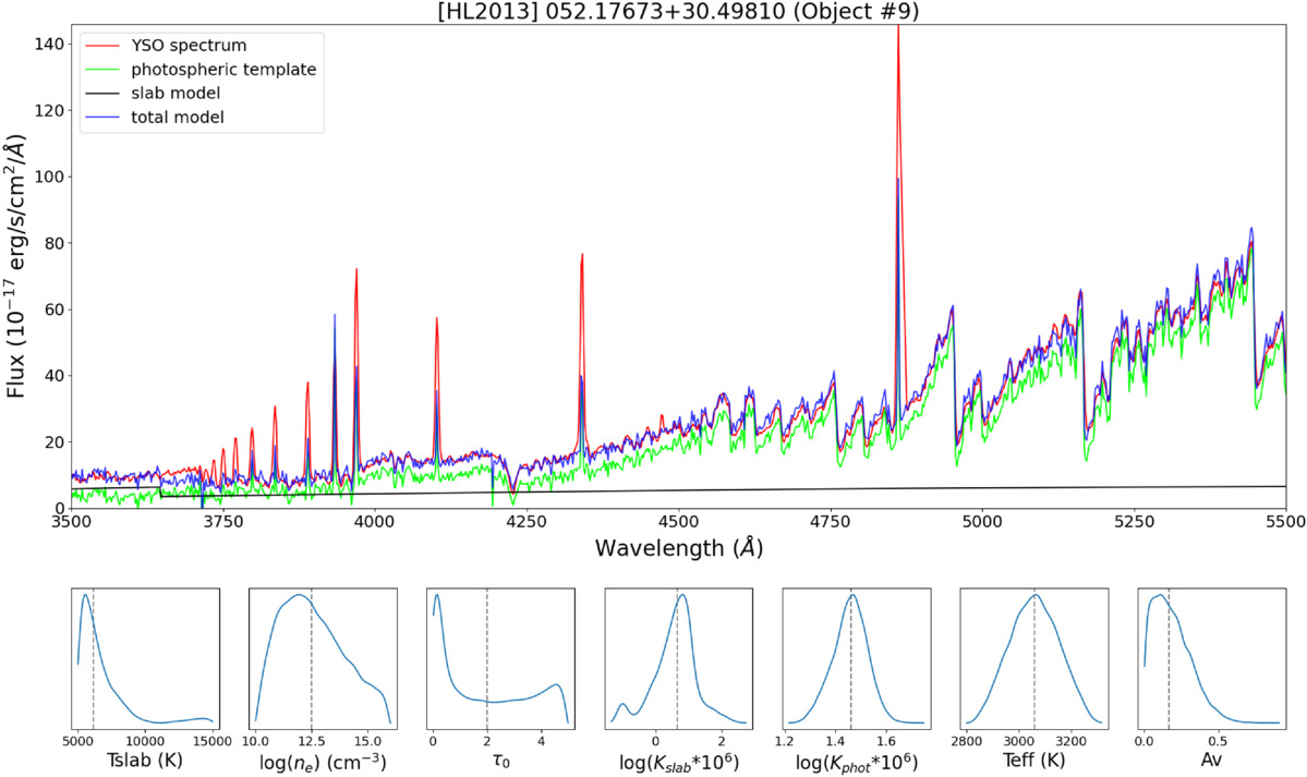
Figure 37. The median model fit for Object 9 and the parameter posteriors with the same plotting convention as Figure 21.
Download figure:
Standard image High-resolution image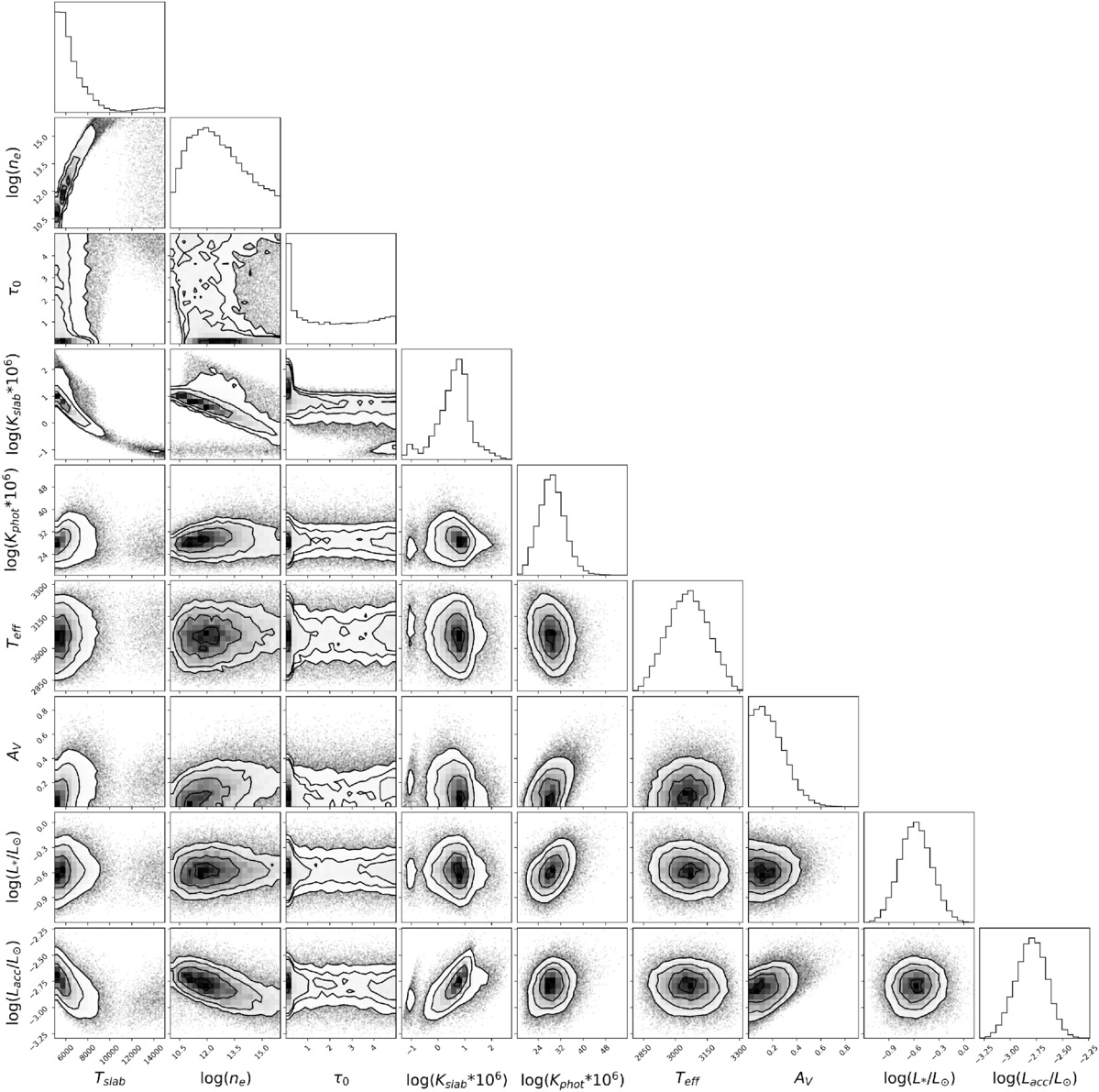
Figure 38. The corner plot for Object 9, for model parameters and the log(L*) and log(Lacc) posteriors.
Download figure:
Standard image High-resolution image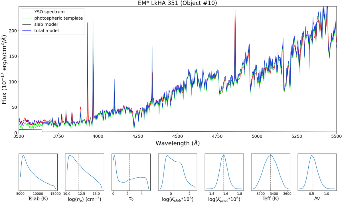
Figure 39. The median model fit for Object 10 and the parameter posteriors with the same plotting convention as Figure 21.
Download figure:
Standard image High-resolution image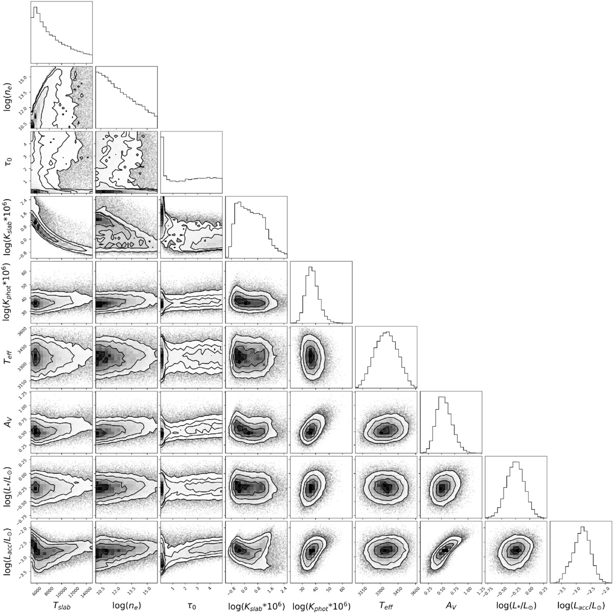
Figure 40. The corner plot for Object 10, for model parameters and the log(L*) and log(Lacc) posteriors.
Download figure:
Standard image High-resolution image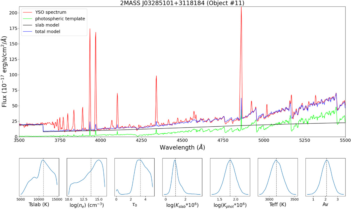
Figure 41. The median model fit for Object 11 and the parameter posteriors with the same plotting convention as Figure 21.
Download figure:
Standard image High-resolution image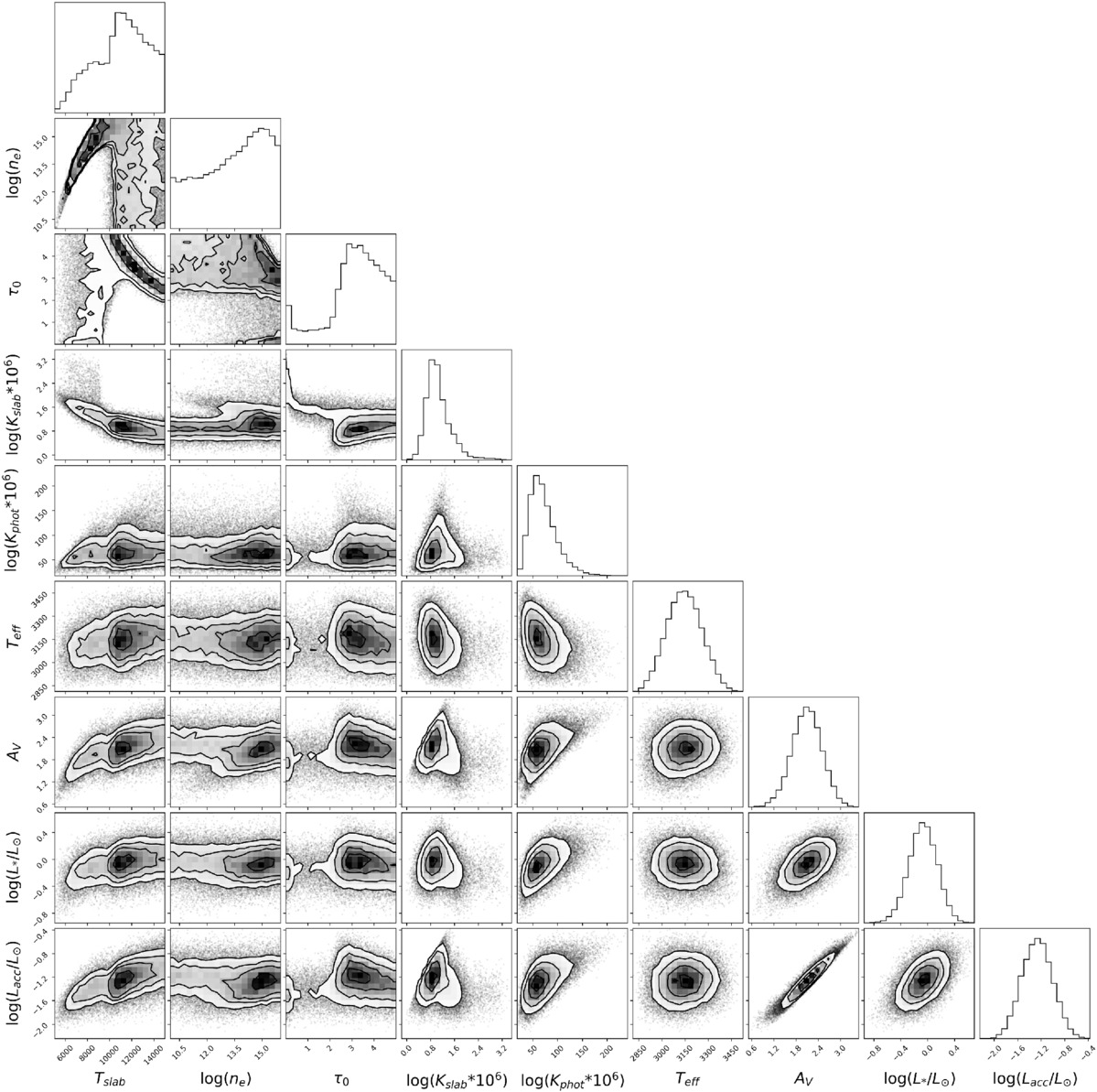
Figure 42. The corner plot for Object 11, for model parameters and the log(L*) and log(Lacc) posteriors.
Download figure:
Standard image High-resolution image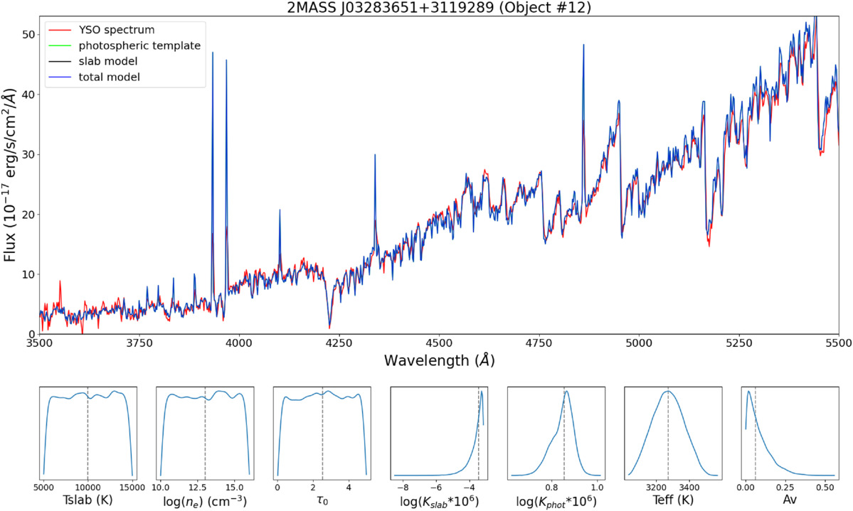
Figure 43. The median model fit for Object 12 and the parameter posteriors with the same plotting convention as Figure 21.
Download figure:
Standard image High-resolution image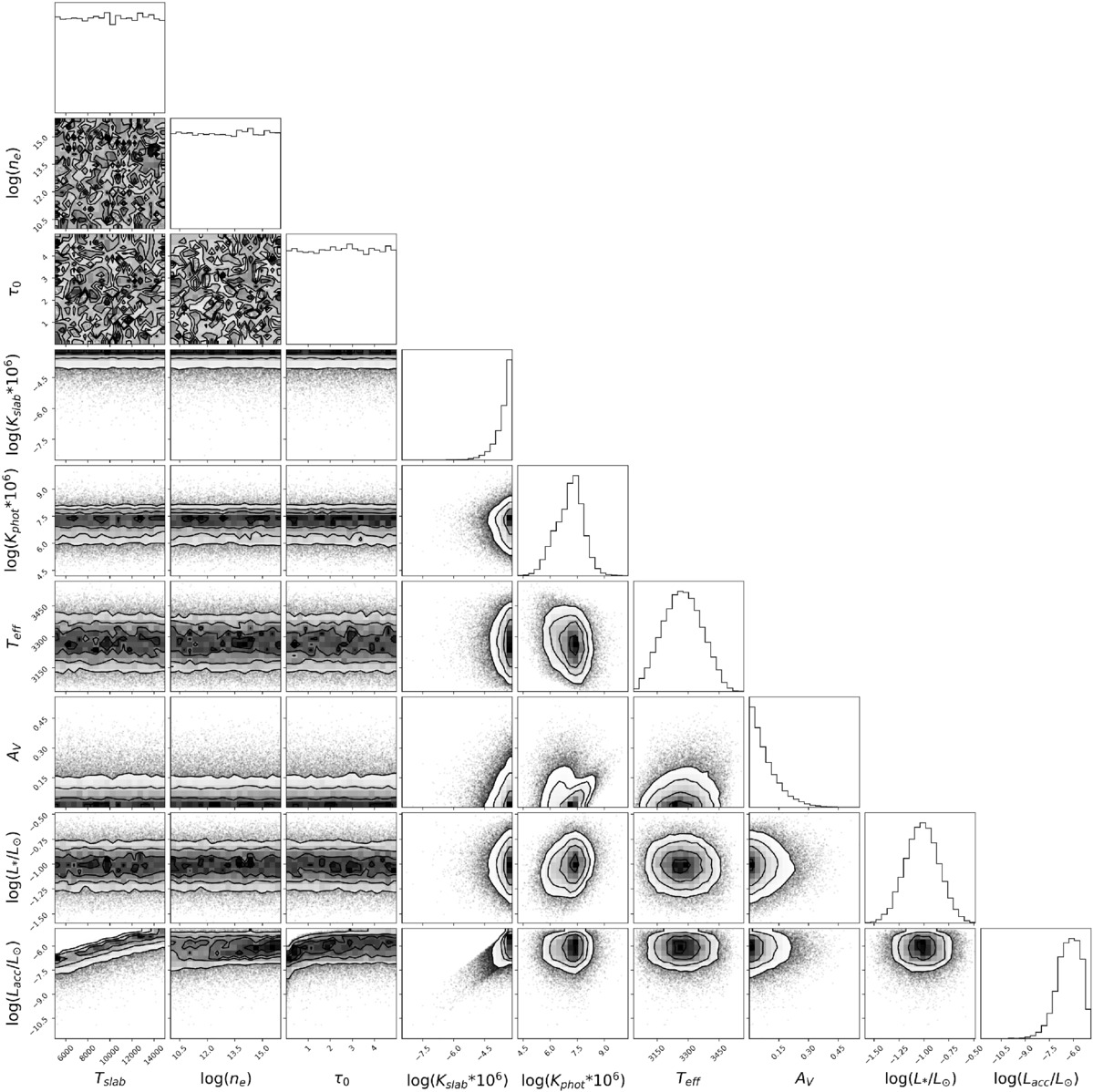
Figure 44. The corner plot for Object 12, for model parameters and the log(L*) and log(Lacc) posteriors.
Download figure:
Standard image High-resolution image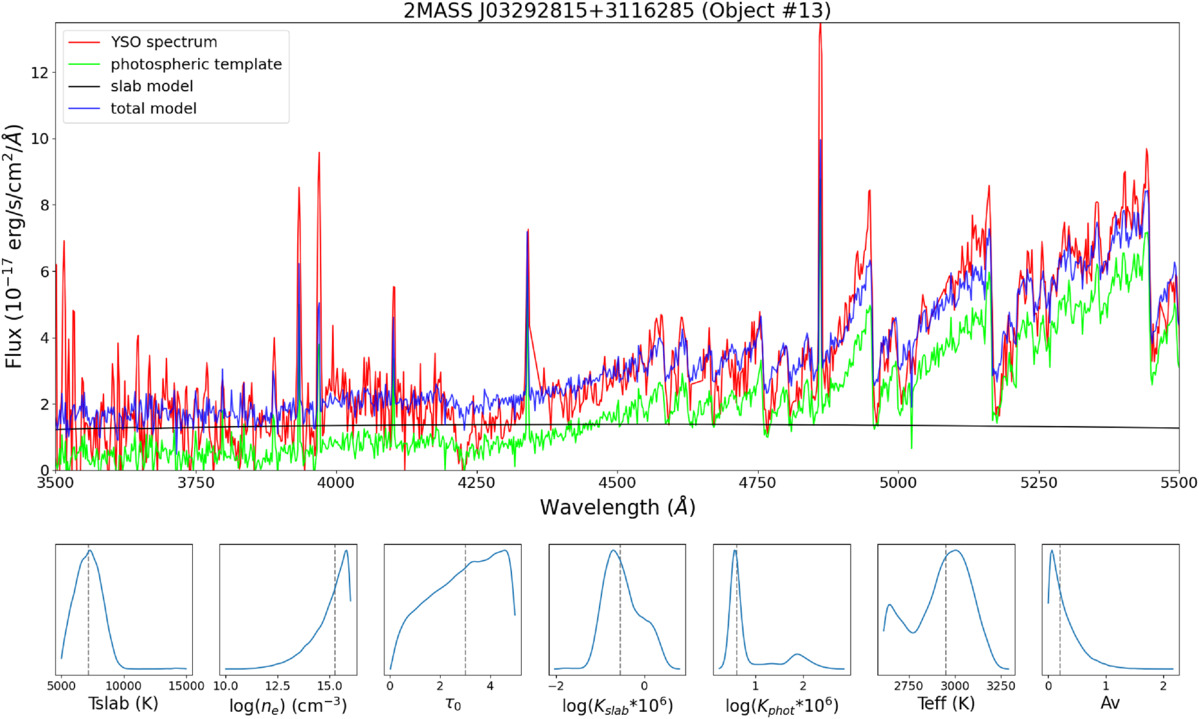
Figure 45. The median model fit for Object 13 and the parameter posteriors with the same plotting convention as Figure 21.
Download figure:
Standard image High-resolution image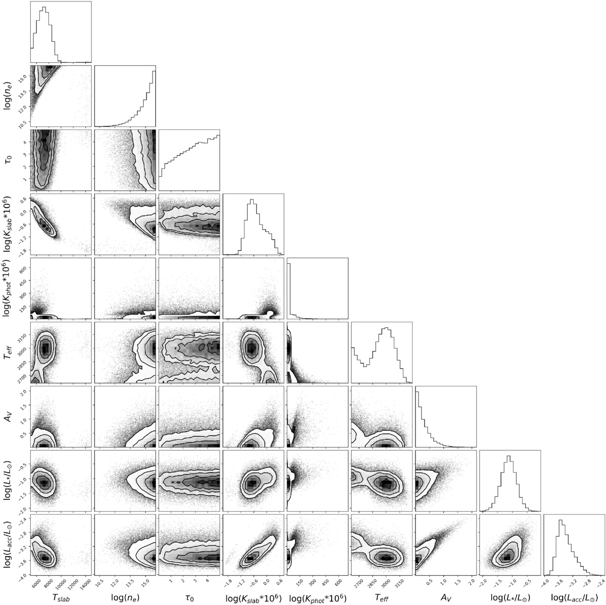
Figure 46. The corner plot for Object 13, for model parameters and the log(L*) and log(Lacc) posteriors.
Download figure:
Standard image High-resolution image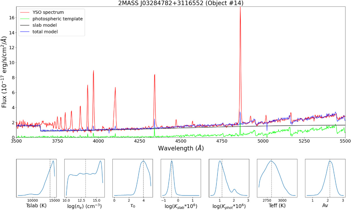
Figure 47. The median model fit for Object 14 and the parameter posteriors with the same plotting convention as Figure 21.
Download figure:
Standard image High-resolution image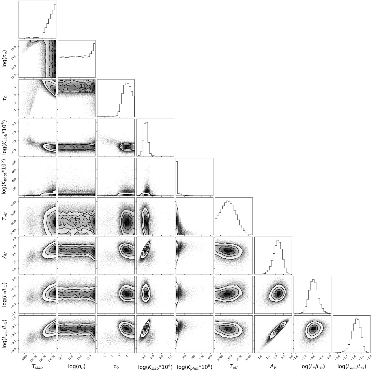
Figure 48. The corner plot for Object 14, for model parameters and the log(L*) and log(Lacc) posteriors.
Download figure:
Standard image High-resolution image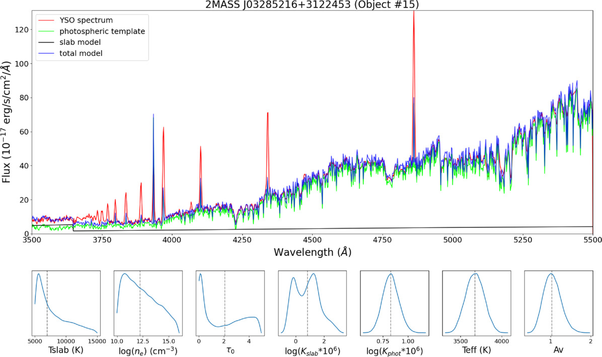
Figure 49. The median model fit for Object 15 and the parameter posteriors with the same plotting convention as Figure 21.
Download figure:
Standard image High-resolution image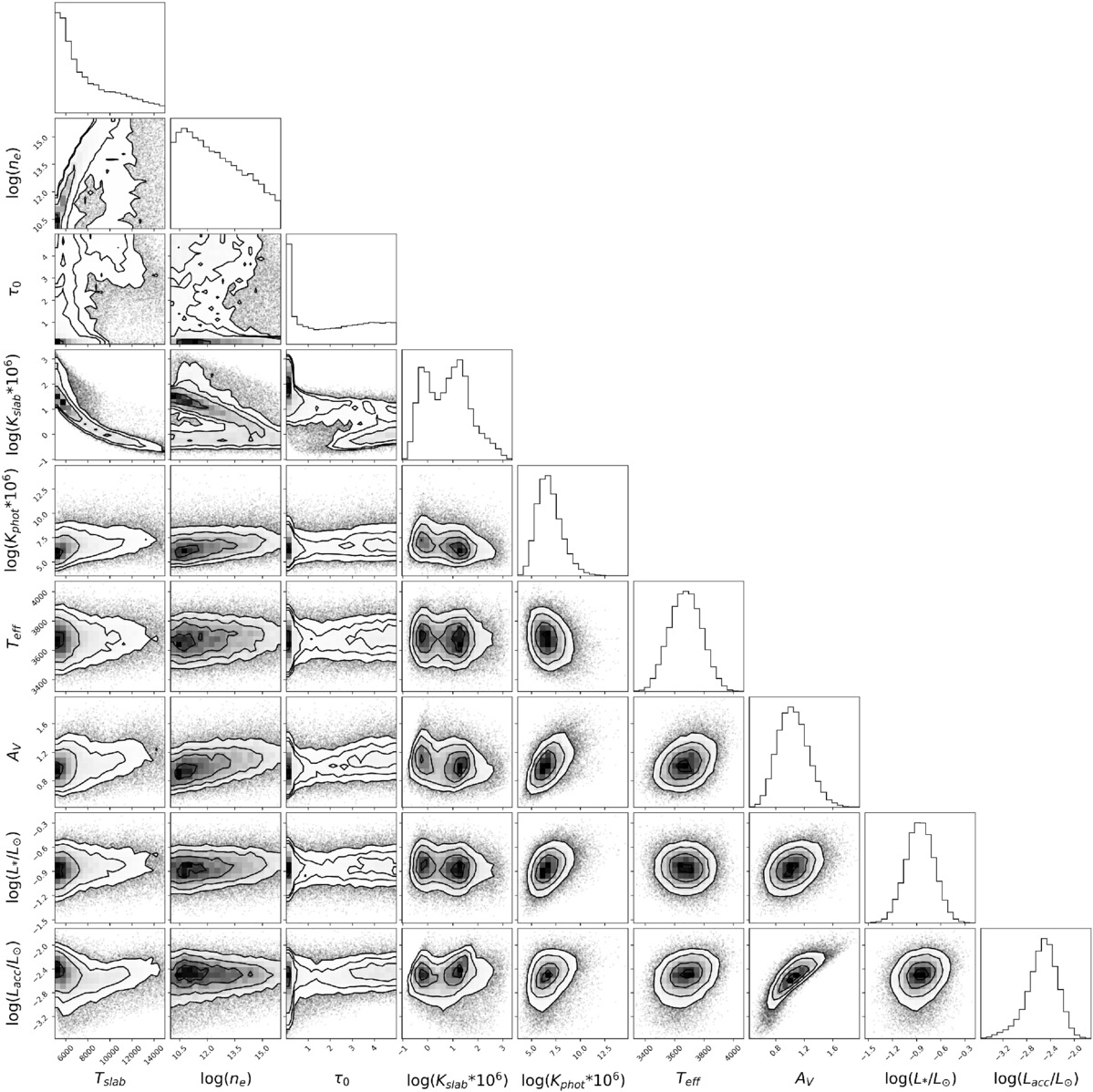
Figure 50. The corner plot for Object 15, for model parameters and the log(L*) and log(Lacc) posteriors.
Download figure:
Standard image High-resolution imageFootnotes
- *
Based on observations obtained with the Hobby-Eberly Telescope (HET), which is a joint project of the University of Texas at Austin, the Pennsylvania State University, Ludwig-Maximilians-Universitaet Muenchen, and Georg-August Universitaet Goettingen. The HET is named in honor of its principal benefactors, William P. Hobby and Robert E. Eberly.
- 8
GAIA EDR3 data can be found at doi:10.5270/esa-1ugzkg7
- 9
- 10
- 11
- 12
- 13
- 14
Data from HST ULYSSES can be found in MAST at doi:10.17909/t9jzeh-xy14.
- 15
- 16
- 17
Pan-STARRS1 DR2 data can be found in MAST at doi:10.17909/s0zg-jx37.