Abstract
The High Cadence Transient Survey (HiTS) aims to discover and study transient objects with characteristic timescales between hours and days, such as pulsating, eclipsing, and exploding stars. This survey represents a unique laboratory to explore large etendue observations from cadences of about 0.1 days and test new computational tools for the analysis of large data. This work follows a fully data science approach, from the raw data to the analysis and classification of variable sources. We compile a catalog of ∼15 million object detections and a catalog of ∼2.5 million light curves classified by variability. The typical depth of the survey is 24.2, 24.3, 24.1, and 23.8 in the u, g, r, and i bands, respectively. We classified all point-like nonmoving sources by first extracting features from their light curves and then applying a random forest classifier. For the classification, we used a training set constructed using a combination of cross-matched catalogs, visual inspection, transfer/active learning, and data augmentation. The classification model consists of several random forest classifiers organized in a hierarchical scheme. The classifier accuracy estimated on a test set is approximately 97%. In the unlabeled data, 3485 sources were classified as variables, of which 1321 were classified as periodic. Among the periodic classes, we discovered with high confidence one δ Scuti, 39 eclipsing binaries, 48 rotational variables, and 90 RR Lyrae, and for the nonperiodic classes, we discovered one cataclysmic variable, 630 QSOs, and one supernova candidate. The first data release can be accessed in the project archive of HiTS (http://astro.cmm.uchile.cl/HiTS/).
1. Introduction
Astronomy has entered the time domain era, with large surveys that monitor the sky for several years aiming to study time variations of astronomical sources. Surveys like MACHO (Alcock et al. 1993), OGLE (Udalski et al. 1992), EROS (Aubourg et al. 1993), and ASAS (Pojmanski 1997) have been used to discover new classes of variable sources and reach a better understanding of their properties and physical nature. These projects were designed with a specific scientific goal, such as the study of microlensing events as a signature of massive compact halo objects, which could explain dark matter, as in the case of MACHO (Cook et al. 1995), OGLE (Udalski et al. 1994), and EROS (Grison et al. 1995). Not only were microlensing events discovered, but a large sample of RR Lyrae, eclipsing binaries, Cepheids, and long-period variables, among others, were also discovered. This led to a better calibration of period–luminosity relations and therefore more accurate distance estimators in the local universe; see, e.g., Sesar et al. (2017).
Presently, there are surveys that are reaching deeper observations, searching for variable stars in the outer halo of our Galaxy and in dwarf satellite galaxies of the Milky Way (MW). All of this is thanks to new astronomical facilities: medium- to large-sized telescopes equipped with large field-of-view instruments like the Dark Energy Camera (DECam; Flaugher et al. 2015) at the 4 m Blanco telescope. The key quantity that measures the survey capabilities of a telescope is etendue, which is the product of mirror collecting area and field of view. Current surveys are focused on transients and variables in general, like the Catalina Surveys (Drake et al. 2009), the La Silla-Quest Variable Survey (Hadjiyska et al. 2012), the QUEST-La Silla AGN variability survey (Cartier et al. 2015), the Intermediate/Palomar Transient Factory (PTF/iPTF; Law et al. 2009), the SkyMapper Southern Sky Survey (Keller et al. 2007), the Panoramic Survey Telescope and Rapid Response System (PanSTARRS; Chambers et al. 2016), the Korean Microlensing Telescope Network (KMTNet; Kim et al. 2016), Gaia (Gaia Collaboration et al. 2016b), the Hyper Suprime-Cam Subaru Strategic Survey (Aihara et al. 2017), the Vista Variable in the Via Lactea (VVV; Minniti et al. 2010), and others. All of these current projects are delivering huge amounts of raw data that need to be processed by taking advantage of the available computational resources: high-performance computing (HPC) to store, manage, and analyze data of the order of terabytes; data visualization tools to analyze high-dimensional data; machine-learning (ML) algorithms to perform automatic classifications; and more. These surveys are laboratories for the next generation of time domain instruments, such as the Large Synoptic Survey Telescope (LSST; LSST Science Collaboration et al. 2009) and the Zwicky Transient Factory (ZTF; Bellm 2014). The data streams will scale exponentially, approximately following Moore’s law (data volume doubles approximately every 2 yr); therefore, a more data science–driven methodology must be implemented to extract the astrophysical knowledge. In particular, the combination of high cadence and large etendue observations represents a perfect combination to search for transients and variable sources with short characteristic timescales such as supernovae, RR Lyrae, nearby asteroids, close eclipsing binaries, and new types of transients.
The ML methods have demonstrated their capability to provide solutions to various astronomical challenges. Important tasks such as classification of galaxies and stars using either photometric data (Ball et al. 2006; Vasconcellos et al. 2011; Kim et al. 2015) or images (Kim & Brunner 2017), classification of variable sources from time-series data (Richards et al. 2012; Pichara & Protopapas 2013; Lochner et al. 2016; Pichara et al. 2016), regression and model fitting algorithms (Ball et al. 2007; Cavuoti et al. 2015; D’Isanto & Polsterer 2018), classification of transient events (Mahabal et al. 2008; Bloom et al. 2012; du Buisson et al. 2015; Förster et al. 2016; Wagstaff et al. 2016; Cabrera-Vives et al. 2017), and detection of anomalous events such as new variability classes (Nun et al. 2016) or unknown spectral signatures (Baron & Poznanski 2017; Solarz et al. 2017; Reis et al. 2018) represent some important examples. One of the advantages of using these methods compared to traditional methods of classification is when data complexity is high. The ML algorithms naturally deal with complex scenarios, not only in terms of the data volume but also in the dimensionality of the problem (e.g., size of the feature space or resolution of the data). Nevertheless, not everything is straightforward when ML algorithms are used. One of the more common problems happens when supervised learning is applied. In the supervised approach, a model is trained with previously labeled data, and then the model is applied to new unlabeled data. Therefore, a key aspect of ML is having a representative training set of the problem. This becomes difficult when new regimes of the parameter space are explored. For instance, in the analysis of time series from photometric data, this could correspond to deeper observations, new filters, or the search for a new type of transient. Thus, one of the main challenges for ML applied in the astronomical domain is creating these training sets to be used with upcoming data.
In this article, we present two science products: a public catalog of detected point-like nonmoving sources and an automatic classification of a catalog of variable stars in the High Cadence Transient Survey (HiTS) database. HiTS was designed to find and study the early phases of supernova events using the DECam imager at the 4 m Blanco telescope at the Cerro Tololo Inter-American Observatory (CTIO). We explain the source extraction and calibration process using standard calibrations and a comparison with public catalogs. We also present a statistical analysis of these catalogs and their structure. Finally, we follow an ML approach to automatically classify light curves according to their variability. In this final part, we address the difficult task of constructing training sets. We explain the different strategies that were used following standard astronomical procedures like catalog cross-matching and visual inspection, modern ML techniques like active learning (AL) and transfer learning (TL), and data augmentation techniques based on transformations to the existing data in the labeled set.
The structure of this paper is as follows. In Section 2, the survey is presented. In Section 3, the pipeline structure is described: preprocessing, catalog creation, astrometric and photometric calibrations, and database structure. In Section 4, we perform an automatic classification of the detected objects using light-curve features, training set construction, and classifier validation and classification. In Section 5, the classification results are presented, and we discuss the encounter biases. Finally, in Section 6, the conclusions of this work are presented.
2. Observations
The HiTS survey (Förster et al. 2016) consists of three observational campaigns in 2013, 2014, and 2015 aiming to study the early phase of supernova explosions. Due to this goal, the survey was designed to have a relatively high cadence, large field of view, and high limiting magnitude. This combination of high cadence and large etendue offers a unique opportunity to do science other than supernova studies, such as studies of moving objects (Peña et al. 2018), studies of distant RR Lyrae stars (Medina et al. 2017, 2018), and variability studies in general.
In this work, we analyze data from all of the 2013, 2014, and 2015 observational campaigns. In 2013, we observed 120 deg2 in 40 fields during four consecutive nights, using an exposure time of 173 s four times per night with a cadence of 2 hr in the u band. In 2014, we observed 120 deg2 in 40 fields during five consecutive nights, using an exposure time of 160 s four times per night with a cadence of 2 hr in the g band. In 2015, we observed 150 deg2 in 50 fields (with an overlap of 14 fields with 2014) during six consecutive nights, using an exposure time of 86 s five times per night with a cadence of 1.6 hr, mostly in the g band but also including r- and i-band observations. In 2014 and 2015, we also had imaging follow-up observations after the main run following an approximately logarithmic spacing in time. For more details of the survey, see Förster et al. (2016).
3. Data Reduction
The preprocessing was performed using a modified version of the DECam community pipeline (DCP; Valdes et al. 2014) that performs electronic bias calibrations, cross-talk corrections, saturation masking, bad-pixel masking and interpolation, bias calibration, linearity correction, flat-field gain calibration, fringe pattern subtraction, bleed trail, edge bleed masking, and interpolation. Cosmic rays were removed using a modified parallel version of CRBLASTER (Mighell 2010), which uses a Laplacian filter (van Dokkum 2001). We removed the DECam CCDs with known issues, N30, S30, and S7, in all fields.11 The main difference between the data reduction process in this work and that in Förster et al. (2016) is the use of images from individual epochs instead of subtracted images.
3.1. Source Extraction
Detection and extraction of sources were performed using SExtractor (Bertin & Arnouts 2010) due to its speed, ease of implementation, and ubiquitous use. A fine-tuning of the parameters was done in order to go as deep as possible while keeping a false-positive rate of detections in single-frame images of less than 1.5% and to perform well in point-like sources. This was done by comparing the single-frame catalogs with those built from deeper stacked images, as explained in Section 3.4. We report fixed-aperture photometry using aperture diameter equal to multiples of the image quality (IQ), defined as half of the empirical full width at half maximum (FWHM) of the image, as well as Kron aperture photometry for extended sources, although SExtractor parameters were not optimized for this purpose. The SExtractor configuration parameters are presented in Table 1.
Table 1. SExtractor Input Parameters
| Parameter | Value |
|---|---|
| ANALYSIS_THRESH | 1.5 |
| BACK_SIZE | 64 [pixels] |
| DETECT_MINAREA | 3 [pixels] |
| DETECT_THRESH | 1.3 |
| GAIN | 4.025 [electrons ADU–1]a |
| PHOT_AUTOPARAMS | [2.5, 3.5] |
| PIXEL_SCALE | 0.27 [arcsec pixel–1]a |
| SATUR_LEVEL | 44,144 [ADUs]a |
| WEIGHT_GAIN | YES |
| WEIGHT_TYPE | MAP_VAPb |
Notes.
aRead from image header. bIf available; if not, WEIGHT_GAIN is used.Download table as: ASCIITypeset image
3.2. Astrometric Calibrations
Output catalogs from SExtractor were astrometrically calibrated against the Gaia DR1 catalog (Gaia Collaboration et al. 2016a) using the latest version of the Software for Calibrating Astrometry and Photometry (SCAMP v2.6; Bertin 2006). The latest version of SCAMP takes into account the full mosaic image from DECam to achieve the astrometric solution. As a comparison, we perform cross-matching with the Gaia and PanSTARRS Data Release 1 (PS1) catalogs. The rms of the residuals is on the order of 0.08 and 005, respectively, with 99% of the cross-matched sources within 0
5 of their matching object.
3.3. Photometric Calibrations
We adopt two different photometric calibration strategies, depending on whether there is information from the PS1 reference catalog in the same filter of our observations. If available, we calibrate all epochs against PS1. If not available, we calibrate all epochs relative to a reference epoch with good observational conditions that are assumed to be photometric for computing zero points (ZPs). We will call these calibration strategies C1 and C2, respectively.
The problem of photometric calibrations can be considered from the point of view of their relative and absolute calibration accuracy. We have found that in those fields where PS1 is available, C1 or C2 gives the same quality of relative photometry. However, C1 gives significantly better absolute photometric calibrations than C2. For 2014 and 2015, we calibrate all epochs using C1, whereas for 2013, we use C2. In what follows, both strategies are described in detail.
C1.—The absolute calibration against PS1 was performed by fitting ZPs for every field, CCD, band, photometry type (Kron and aperture), and epoch. We calculate the ZPs on cross-matched objects between the PS1 and HiTS catalogs with magnitudes between 16 and 21 for the g band and between 16 and 20 for the r and i bands. This is due to the difference in depths and observing conditions encountered when observing each band, namely airmasses or sky brightness. We applied a σ-clipping filter of three times the median absolute deviation around the median of the magnitude difference distribution to remove outliers. The ZP values were calculated as the median value of the magnitude difference for sources that remained after filtering. We estimated uncertainties on ZPs using bootstrapping to sample from the distribution of filtered magnitude differences. We tested these results against a Monte Carlo Markov chain (MCMC) method assuming a model with the ZP and its error as parameters. The MCMC posterior median error was, on average, 16% larger than the bootstrap error. Thus, we report ZP uncertainties as 1.16 times the bootstrap error. Finally, reported magnitudes for detected sources are corrected by the ZP calculated as


where m is the calculated AB magnitude, F is the SExtractor measured flux in analog-to-digital units (ADUs), texp is the exposure time of the observation, ZP is the ZP mentioned above, δm is the calculated photometric uncertainty, δF is the measured flux error (from Equation (7) as explained next) in ADUs, and δZP is the uncertainty of the ZP.
C2.—We applied relative flux calibrations with respect to a reference epoch, which was chosen to be the best in terms of seeing for every field and CCD. We fitted a linear relation between the fluxes of the same stars in the nonreference versus reference epochs and applied a transformation to the fluxes in the nonreference epochs:  , where
  is the transformed flux, Fi is the original flux, and aflux is the slope of the fitted relation. Then, all fluxes are converted to magnitudes following the DECam photometric standard calibration, ignoring color terms, since the relevant colors are not available:


where F′ is the transformed flux mentioned above in ADUs, X is the observed airmass, A and K are the ZP and airmass coefficients from the DES science verification archive,12 δF′ is the transformed flux error in ADUs, and δA and δK are the reported uncertainty of the ZP and airmass coefficients.
In order to estimate the uncertainties δF of the measured fluxes, we use corrected SExtractor errors. It is well known that errors from SExtractor are generally underestimated (Labbé et al. 2003; Gawiser et al. 2006). SExtractor estimates errors using the following relation (Bertin & Arnouts 2010):

where σ1 is the typical fluctuation per pixel (mostly due to sky Poisson noise), npix is the number of pixels within the aperture, F is the measured flux, and GAIN is the effective gain used to convert ADUs into detected photons. The first term represents the sky fluctuations assuming uncorrelated noise between pixels, and the second term is the Poisson variance or shot noise from the source. One way to include the noise correlation is to empirically study background fluctuations as a function of the aperture size using randomly located circular apertures with a range of aperture diameters (Gawiser et al. 2006). In Figure 1 (top panel), we show the distribution of flux measurements of background-subtracted images for 1000 randomly located apertures with different effective sizes N. Then, we model the uncertainties to be proportional to the number of pixels of the aperture to a given power β,

where N is the effective size of the aperture ( ). In Figure 1 (bottom panel), we show the empirical relation (circles) and the extreme cases of no correlation and perfect correlation that correspond to ∼N and ∼N2, respectively.
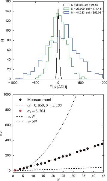
Figure 1. Top: distribution of measured flux on randomly located apertures for three effective sizes N; the fluxes were measured on the background-subtracted image. Bottom: background fluctuations as a function of aperture size. Circles represent the empirical variation on images of field Blind15A_25, CCD N1; the red dashed line represents the fitted function with α = 0.850 and β = 1.133. The black dashed lines represent the extreme cases of independent noise from pixel to pixel and correlated noise from fluctuations in background level that leads to an rms proportional to N and N2.
Download figure:
Standard image High-resolution imageFinally, the uncertainties of the measured fluxes are given by

where α and β are given in Equation (6) and npix is the number of pixels within the aperture. For the Kron aperture on SExtractor, the area is given by the Kron best-fit ellipse. Then, the number of pixels within the Kron aperture is given by  , where rKron is the Kron radius and A_IMAGE and B_IMAGE are the major and minor axes of the ellipse, respectively. For fixed circular apertures, the number of pixels is given by npix = π × (k × IQ)2, where k is an integer.
3.4. Survey Depth
In order to calculate the completeness magnitude of our catalogs, we created deep images combining the 10 best epochs per campaign. Catalogs were extracted from stacked images and then compared against catalogs from single-epoch images. Assuming that at the depth of the single images, the stacked images were complete (in terms of detectable sources), we compared the magnitude distribution from both catalogs to obtain the magnitude at a given completeness level. In the top panel of Figure 2, the black and blue lines represent the distribution of detected sources in the stack and single-epoch images, respectively. It is easy to see that at the bright end (left), the ratio is consistent with 1 (see bottom panel), but around 23 mag, this ratio decreases, reaching 50% at 23.8 mag.
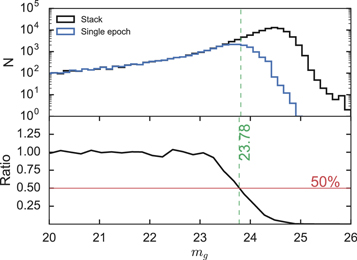
Figure 2. Top: distribution of detected sources. The black histogram represents all detections in the stack image, and the blue histogram represents sources from the single-epoch catalog with a match between both. Bottom: ratio of both distributions representing the detection recovery. The horizontal red line represents the 50% level of completeness; this is achieved at ∼23.8 mag for a typical field in the g band.
Download figure:
Standard image High-resolution imageIn order to calculate the limiting magnitudes per field and epoch, we measured the flux fluctuations of randomly located empty apertures using the standard deviation of 1000 aperture fluxes where no sources were detected. Then, assuming a signal-to-noise ratio (S/N) of 5 for detection, we determined the limiting magnitudes per field, CCD, and epoch as five times the previous standard deviations.
Figure 3 shows (bottom panels) the evolution along epochs of g-band limiting (solid black line) and completeness (dashed blue line) magnitudes for observations during 2013, 2014, and 2015. The top panels show the evolution of the observed airmass and measured FWHM in arcseconds. In all three years, the limiting and completeness magnitudes follow the airmass evolution within the night. Figure 3(c) shows an increase of the measured FWHM between epochs 15 and 25; this is due to observations during two cloudy nights having a severe impact in the limiting magnitudes.
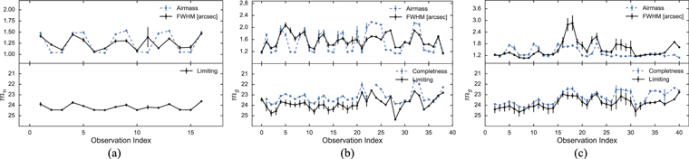
Figure 3. Panels (a), (b), and (c) refer to observation campaigns during 2013, 2014, and 2015, respectively. Evolution of the observed airmass (dashed blue line) and measured FWHM (solid black line) in arcseconds are given in the top panel. Derived completeness and limiting magnitude are shown in the bottom panel, both as a function of epoch number.
Download figure:
Standard image High-resolution imageThe rate of detections that are nonreal sources, i.e., the false-positive rate of detections, was also derived comparing catalogs from stacked and single-epoch images, which were found to be at the level of 1% at magnitude 23.8 (only considering point-like sources). Therefore, our catalogs are typically at least 99% pure at the completeness magnitude.
In order to test the quality of our photometric errors, we compared the flux standard deviation with the median photometric uncertainty for every source. In Figure 4, we show the empirical standard deviation versus the median estimated photometric uncertainty. We found that the previous standard deviations are of the same order as the estimated median errors (combining SExtractor, pixel correlation, and ZP uncertainty). However, the distribution of the ratio between the previous two quantities has a median of about 1.3. An increased empirical standard deviation could be due to several factors: the contribution of the more noisy epochs due to varying observational conditions; the correction in Equation (7), which does not take into account correlated noise coming from the source; and the contribution of intrinsically variable sources. Thus, the ratio between empirical standard deviations and the estimated uncertainties is expected to be greater than 1.
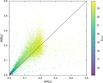
Figure 4. Standard deviation of detections vs. median photometric uncertainty, color-coded by median magnitude for a typical field during the 2015 g band. The diagonal line is the identity representing variations in the photometry similar to its error; significant departures from the identity are due to intrinsic variability and insufficient correction by pixel correlations.
Download figure:
Standard image High-resolution imageFurther comparisons of HiTS against the PS1 photometric catalogs are shown in Figure 5 for all three filters available in the 2015 data. In the g band, the relation is close to the identity with a small scatter of the order of 0.02 mag up to 21.5 mag. Above 21.5 mag, where the HiTS catalog is 3 mag and PS1 is 2 mag below their completeness magnitudes, PS1 values tend to be underestimated compared to the HiTS photometry. For the r and i bands, the conclusions are similar, but the scatter is of the order of 0.04 and 0.07 mag, respectively.
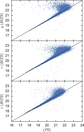
Figure 5. HiTS against PS1 photometry for the g, r, and i bands (top, middle, and bottom panels, respectively). The scatter around the identity for relatively bright sources, up to 21.5, is of the order of 0.02, 0.04, and 0.07 for the g, r, and i bands. Beyond 21.5 mag, the scatter from the identity increase, we claim that PS1 values tend to be underestimated compared to HiTS photometry, mainly due to the single-epoch depth of both surveys, where HiTS reaches the completeness magnitude at ∼24 and PS1 at ∼23.
Download figure:
Standard image High-resolution image3.5. Catalogs and Database
In total, we obtained 1,980,107 detected sources in the u band for 2013 and 5,389,028 sources in the g band for 2014. For the 2015 observations, we obtained 5,117,233 sources in the g band, 5,884,126 in the r band, and 4,572,003 in the i band. Due to the overlap of 14 fields between the 2014 and 2015 observation campaigns, 1,190,008 sources have been cross-matched using a radius of 0.5 arcsec between both catalogs. The number of single-epoch detections for all three campaigns is about 100 million. The structure of this catalog is similar to the structure used in PS1. The column description of the catalogs is presented in Appendix A (see Table 5). Public catalogs are available and accessible in the project archive of HiTS13 ; DR1 has also been archived on Zenodo (doi:10.5281/zenodo.1410651 ). The database is available as compressed tarball files for the entire HiTS survey and also separated by fields. In the future, we will test the possibility of using a dedicated time-series database (e.g., influxDB14 ) to store and access the data.
4. Automatic Classification
The typical procedure to perform a supervised automatic classification using ML algorithms is the following. First, build a labeled set with the desired classes in a subset of the entire database; this can be accomplished by running a cross-match with available public databases. Then, train a supervised classifier with a subset of the labeled set (the training set). Then, the model is validated with a subset of the labeled set that was not used to train (the test set). Finally, a prediction is made on the unlabeled data. In our case, we use a feature engineering approach, i.e., to represent each time series as a user-defined feature vector and with labels corresponding to variability classes of the astronomical sources.
We clean the detection catalog to remove extended sources, and we filter by FWHM, Ellipticity, FluxRadius, and KronRadius to select point-like sources. Afterward, we filter out saturated sources at the bright end of the magnitude distribution. Finally, we select all sources with more than 15 detections to build their light curves and perform the automatic classification by variability. We end up with 2,536,100 point-like sources after the selection mentioned above for the 2014 and 2015 data.
4.1. Feature Extraction
We extract features using the feature analysis for time series (FATS; Nun et al. 2015). Some of these features are mean, standard deviation, amplitude, period of the Lomb–Scargle periodogram maximum, false-alarm probability of the period, mean variance, and median absolute deviation. The full list of features is shown in Table 8 in Appendix B. Note that the set of features has already been used in other works (Mackenzie et al. 2016; Nun et al. 2016; Pichara et al. 2016). We also added periods calculated using both the generalized Lomb–Scargle technique (GLS; Zechmeister & Kürster 2009) and correntropy kernel periodogram (CKP; Huijse et al. 2012), as well as color indices calculated when observations were available (g, r, and i bands).
4.2. Labeled Set
In order to build a labeled subset with the astronomical variability classes expected to appear in our survey, we considered three approaches: cross-match with public catalogs, visual inspection, and TL combined with AL.
The first and more standard approach is to run a cross-match with public catalogs of variable sources. However, due to the uniqueness of our survey in terms of cadence, depth, and survey area, other surveys tend to have a small overlap with HiTS. Surveys such as MACHO, EROS, and OGLE do not overlap spatially with HiTS. We found overlap with the Sloan Digital Sky Survey Data Release 9 (SDSS DR9; Ahn et al. 2012), the General Catalog of Variable Sources (GCVS; Samus et al. 2009), the Catalina Sky Survey Data Release 1 (CSDR1; Drake et al. 2014), and the International Variable Star Index (VSX; Watson 2006). We also included a comparison with parallel searches for RR Lyrae and supernovae on the same data (Förster et al. 2016; Medina et al. 2018, respectively). It is important to notice that the low number of positive cross-matched sources (about 30) between our light curves and the supernovae detected by Förster et al. (about 120 detections) is due to the methodology used. We detect sources with SExtractor in the direct images, while Förster et al. used image differences that perform better near the core of the galaxy host. The classes and number of cross-matched sources from each different survey are summarized in Table 2.
Table 2. Summary of Number of Objects per Class from Different Approaches to Building the Labeled Set
| Source | NV | QSO | CV | RRLYR | EB | MISC | SNe | LPV | RotVar | ZZ | DSCT | Total |
|---|---|---|---|---|---|---|---|---|---|---|---|---|
| SDSS DR9 | ⋯ | 3495 | 85 | ⋯ | ⋯ | ⋯ | ⋯ | ⋯ | ⋯ | ⋯ | ⋯ | 3580 |
| GCVS | ⋯ | ⋯ | 1 | 22 | 1 | ⋯ | ⋯ | ⋯ | ⋯ | ⋯ | ⋯ | 24 |
| CSS | ⋯ | ⋯ | 1 | 26 | 91 | ⋯ | ⋯ | 1 | 5 | ⋯ | ⋯ | 124 |
| VSX | ⋯ | ⋯ | 11 | 126 | 105 | 7 | ⋯ | 1 | 5 | 2 | 1 | 258 |
| Medina et al. (2018) | ⋯ | ⋯ | ⋯ | 60 | ⋯ | ⋯ | ⋯ | ⋯ | ⋯ | ⋯ | ⋯ | 60 |
| Förster et al. (2016) | ⋯ | ⋯ | ⋯ | ⋯ | ⋯ | ⋯ | 29 | ⋯ | ⋯ | ⋯ | ⋯ | 29 |
| Visual inspection | 5000 | ⋯ | ⋯ | ⋯ | ⋯ | ⋯ | ⋯ | ⋯ | ⋯ | ⋯ | ⋯ | 5000 |
| TL and AL | ⋯ | ⋯ | ⋯ | ⋯ | 10a | ⋯ | ⋯ | ⋯ | ⋯ | ⋯ | ⋯ | 10 |
| Totalb | 5000 | 3495 | 94 | 177 | 110 | 7 | 29 | 1 | 5 | 2 | 1 | 8921 |
| Data augmentation | 5000 | ⋯ | ⋯ | 100 | 200 | ⋯ | ⋯ | ⋯ | 179 | ⋯ | 166 | 5645 |
| Labeled setc | 10,000 | 3495 | 94 | 277 | 310 | ⋯ | 29 | ⋯ | 184 | ⋯ | 167 | 14,566 |
Notes. Variability classes are nonvariable (NV), quasar (QSO), cataclysmic variable (CV), RR Lyrae (RRLYR), eclipsing binary (EB), miscellaneous variable (MISC), supernovae (SNe), long-period variable (LPV), rotational variable (RotVar), ZZ Ceti variable (ZZ), and δ Scuti variable (DSCT).
aLater confirmed by cross-match. bTotal values per class might not represent the direct addition of column values; this is due to some objects being present in different catalogs. cRepresents the actual total number of sources per class used during the training and testing tasks.Download table as: ASCIITypeset image
The second approach consists of a visual inspection of light curves from sources that have a low false-alarm probability obtained from their Lomb–Scargle periodogram maximum (i.e., the largest period_fit value given by FATS). We also visualized the light curves of sources with very low variability (std, mean variance, and variability index given by FATS) in order to add them to the nonvariables class of the training set.
After the first two approaches, we end up with 11 classes of variability: nonvariables (NV), quasars (QSO), cataclysmic variables (CV), RR Lyrae (RRLYR), eclipsing binaries (EB), miscellaneous variable stars (MISC), supernovae (SNe), long-period variables (LPV), rotational variables (RotVar), ZZ Ceti variables (ZZ), and δ Scuti variable stars (DSCT).
Due to the small number of instances for some classes after the cross-match, which leads to an unbalanced training set, we tried the third approach of TL combined with AL. Here TL (Qiang Yang 2009) is a method to learn from a training data set that exists in a different domain, the source domain, to train a classifier that will be applied in a different domain, the target domain. For instance, to train a classifier based on V-band light curves that will be applied to g-band light curves. This is particularly useful when a large training set exists in the source domain, but no equivalent set exists in the target domain. Here AL (Settles 2012) is an iterative and interactive process in which expert input is required to classify objects where the classification cannot be done with a high level of confidence and, with this information, improve the classifier. This process is done iteratively until certain criteria are met, e.g., the test set accuracy or the amount of sources per class are satisfactory.
There are already compiled training sets that can be used for the classification of variable stars, such as MACHO, OGLE, and EROS. A TL approach is required to train a classifier for HiTS using these data sets because these surveys were observed with a different band, cadence, and depth and in a different part of the sky (the source domain for TL). A simple way to transfer the labeled sources is to calculate the same features in both the source and target domain and compare their distributions. Then, a simple transformation is found, e.g., scaling and translation, that forces both distributions to be similar. The main problem with this approach is that finding the transformation can be difficult, especially when the distributions of features are very dissimilar. This is our case. The sampling function of HiTS is very different from those of MACHO. MACHO was observed in the BVR filters, but HiTS was observed in the ugri filters; MACHO reached a depth of ∼20 mag in the B band, while the HiTS depth was ∼24.5 mag in the g band; finally, the cadence of MACHO was on the order of days (even weeks) during 5 yr, but that of HiTS was on the order of hours during about a week. The latter is probably the most important difference between these surveys. Therefore, it was not possible to find a simple transformation between both spaces.
We tested a basic combination of TL with AL. A simple transformation was applied to the feature distribution of MACHO to match HiTS, and then a random forest (RF) classifier (see next subsection for a description of the method) was trained using the transformed feature values of MACHO. The hyperparameters of the model were tuned following a cross-validation approach15 within the MACHO training set. For this and further tests, we set a stratified sixfold cross-validator to preserve class unbalance. When classifiers without TL and with our simple transformation were tested on the current HiTS labeled data set (using only labeled sources from cross-matching in Table 2), we found that in the first case, the accuracy was ∼5%, and in the second case, the accuracy improved to ∼15%. None of these classifiers reached a satisfactory level of accuracy. But, predicting in unlabeled HiTS data, we were able to confirm the classification of those objects with the highest classification confidence via visual inspection done by experts and to then add them to the labeled set (basic AL procedure). We performed this method with only one iteration, since most of the newly labeled objects belonged to the already well-populated classes. In those cases, the new objects were not added to the labeled set. The EB sources provided by this method were later confirmed via post-cross-matching with the same catalogs presented above. The contribution of this mixture of TL and AL to the training set is shown in Table 2.
The total amount of items per class shown in Table 2 is too small for some classes—for instance, one and five items for DSCT and RotVar, respectively. In these cases, the classification model does not create a good representation of the classes, leading to unreliable results when cross-validation techniques are used.
In order to compensate the less-populated classes, we follow a data augmentation approach (see, e.g., Dieleman et al. 2015). We use known objects in the periodic classes to create synthetic light curves from them by applying basic transformations (i.e., scaling, noise addition, and phase shifting). To create these synthetic light curves, we follow these steps. We model the observed folded light curves using a Gaussian process (GP; Rasmussen & Williams 2005), which is a nonparametric method to model the data. We use the GP regression implemented in scikit-learn16 with a periodic ExpSineSquare17 kernel; then, we sample from this model following the HiTS observing strategy. At this step, we also apply a transformation in the time coordinate to simulate different periods consistent with the distribution of periods in each class. We remove data points in the dim end of the magnitude distribution to emulate the typical fraction of missed data in the light curves. Mean values are scaled to the HiTS empirical magnitude distribution, adding heteroscedastic noise using the empirical distributions of errors given a magnitude bin. Finally, features are calculated, as was done for real light curves.
Following this method, we were able to increase the population for the RRLYR, EB, DSCT, and RotVar classes (see Table 2). For the transient class, it is more difficult to perform data augmentation because applying time shifts requires a more difficult interpolation and may require extrapolation. For the nonperiodic CV and MISC classes of variable sources, it is also difficult to perform data augmentation. The CVs exhibit quiescence and outburst behavior in a nonperiodic fashion according to their accretion rate with timescales of weeks to years plus timescales of hours due to orbital variations. The MISC class is a heterogeneous family of variable stars and thus difficult to characterize; therefore, we eliminated this class from the training set. For periodic ZZ variables, which are fast-pulsating stars with periods from seconds to dozens of minutes, even the fast cadence of HiTS is not fast enough for their proper characterization. Therefore, the ZZ class was also removed from the training set.
The final training set contains the classes and numbers listed in the last row of Table 2. The catalog with sources and classes used for the classification task is available in the project archive of HiTS (see footnote 13), and the column description of the catalog is presented in Appendix A (see Table 6). Examples of periodic and nonperiodic light curves are shown in Figure 6.
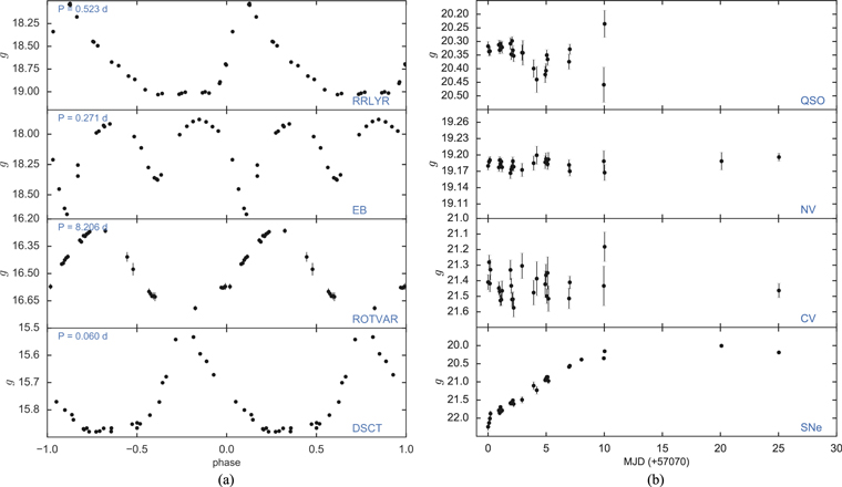
Figure 6. (a) Examples of periodic light curves for objects in the training sample. Light curves are phase folded using period calculation from GLS. (b) Examples of nonperiodic light curves for objects in the training sample.
Download figure:
Standard image High-resolution image4.3. Model Training and Testing
We follow a hierarchical classification scheme using an RF classifier (Breiman 2001). Briefly, RF consists of a collection of single decision-tree classifiers that partition the feature space in a hierarchical fashion, where each tree is trained with a random selection of objects and features, and the final classification is the average outcome of each individual tree. In astronomy, RF has been extensively and successfully used to classify sources (Pichara & Protopapas 2013; Kim et al. 2014; Förster et al. 2016; Yuan et al. 2017). For this work, we use the scikit-learn18 implementation of RF. We set the number of estimators (the number of trees) per classifier and the maximum depth of the trees (the maximum path length at which nodes are no longer expanded), minimizing the out-of-bag error at the training phase (which is the predicted error on a bootstrap aggregation). The remaining hyperparameters of the classifier (such as the split criteria, number of features to learn in each tree, and minimum number of samples per leaf) were set as the best F1-score19 value from the cross-validation process. Class imbalance was taken into account, weighting each class in the training set by initializing the class weight hyperparameter as “balanced_subsample.” We fed all the features listed in Table 8 to the RF model. Each classifier in the hierarchical scheme was tested using an unseen set—the test set—that represented one-third (∼4500) of the full labeled set while maintaining the imbalance of classes. This set was composed of real sources, with the exception of the RotVar and DSCT classes, due to the small number of real objects.
The hierarchical classification allows us a better understanding of the possible contaminants of each class. For the hierarchical scheme, we divide the classification into two binary layers and one final multiclass layer. The first layer consists of a binary variable/nonvariable classification. The NV class was set as a nonvariable class during this step. The QSOs were removed from this layer. The reason for this is that short-term variability (with timescales of hours) is not a well-constrained property of QSOs. Other than blazars, which are well-known fast variables, small samples of a few dozen “normal” QSOs show short-term variability in about ∼10%–30% of objects but with amplitudes of ∼3%–10% (Stalin et al. 2004; Gupta & Joshi 2005). The poorly known properties of this variability could make classification at this stage less reliable.
A confusion matrix presenting our results is shown in Figure 7, where it is easy to see that variables are in general well classified and false positives are statistically zero; i.e., we achieved a high purity. The F1 score on the test set is 99% ± 0.1% (see Table 3 for peer class score values).
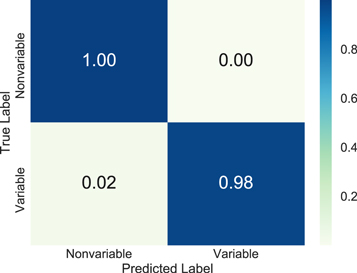
Figure 7. Confusion matrix from testing results for variable/nonvariable classification. True Label represent the ground truth, and Predicted Label is the outcome of the RF classifier.
Download figure:
Standard image High-resolution imageTable 3. Summary of Precision, Recall, and F1 Scores for Every Step in the Hierarchical Classification as Measured in the Test Set
| Variability Class | Precision | Recall | F1 Score |
|---|---|---|---|
| Variable (basic) | 0.92 | 0.97 | 0.95 |
| Nonvariable (basic) | 1 | 0.99 | 0.99 |
| Variable (RF) | 1 | 0.98 | 0.99 |
| Nonvariable (RF) | 1 | 1 | 1 |
| Periodic | 0.99 | 0.99 | 0.99 |
| Nonperiodic | 0.97 | 0.96 | 0.96 |
| DSCT | 0.96 | 0.96 | 0.96 |
| EB | 0.86 | 0.91 | 0.88 |
| RotVar | 0.94 | 0.94 | 0.94 |
| RRLYR | 0.98 | 0.93 | 0.95 |
| CV | 0.88 | 0.96 | 0.92 |
| QSO | 0.89 | 0.82 | 0.86 |
| SNe | 0.80 | 0.67 | 0.73 |
Download table as: ASCIITypeset image
Next, for variable candidates, we separate the periodic and nonperiodic classes. Here the periodic classes are RRLYR, EB, LPV, RotVar, and DSCT, while the nonperiodic classes are CV, SNe, and QSO. Only QSOs that were classified as variable with the variable/nonvariable classifier (described above) are included in this layer as nonperiodic sources; this is 177 out of 3495. We remove all true periodic variables with bad period estimations (i.e., period_fit > 0.5) from the training set. The main reason to do this is the presence of periods longer than weeks in the training set, which are not possible to recover with the HiTS observational time span. This only reduces the number of periodics by 68 sources. The F1 score after doing this is 98% ± 0.1%, and the corresponding confusion matrix is shown in Figure 8. The false-positive rate is around 4%, and the classifier misses only 1% of the periodic sources.
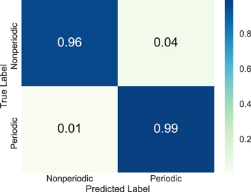
Figure 8. Confusion matrix from testing results for periodic/nonperiodic classification. Similar to Figure 7.
Download figure:
Standard image High-resolution imageFor the final layer, a multiclass classification is applied for each periodic and nonperiodic subset. Within the nonperiodic set, the classifier was trained with three classes (QSO, CV, and SNe), and for the periodic set, it was trained with four classes (RRLYR, EB, RotVar, and DSCT).
For the periodic set classifier, the injection of synthetic light curves significantly improves the performance of the classifier for the RotVar and DSCT classes compared with a classifier trained only with real data: from 14% to 94% and from 0% to 97% for the RotVar and DSCT classes, respectively. However, if we test only with real sources, we recover four out of five sources in the RotVar class (80% recall) and one out of one source in the DSCT class. The EB and RRLYR classes did not show significant improvement after the injection of synthetic light curves. The confusion matrix shown in Figure 9 presents the results of the test set for this layer, where it is possible to notice that, in general, misclassification is below 5% in all classes. The weighted F1 score is 93% ± 2%.
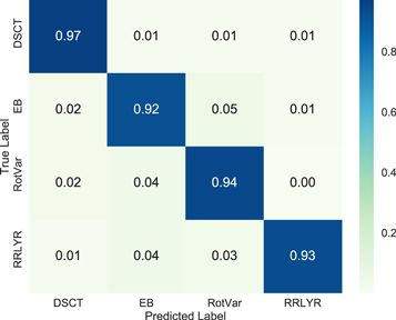
Figure 9. Confusion matrix from testing results for periodic subclass classification. Similar to Figure 7.
Download figure:
Standard image High-resolution imageFor the nonperiodic set, the classes are QSO, CV, and SNe. The weighted F1 score is 88% ± 3%. Figure 10 shows the confusion matrix for this classification model. Here the misclassification is higher, given the short time span of the survey. In many cases, CVs and QSOs are either observed during their quiescent state or have longer characteristic timescales of variability.
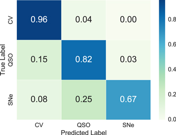
Figure 10. Confusion matrix from testing results for nonperiodic subclass classification. Similar to Figure 7.
Download figure:
Standard image High-resolution imageOne of the advantages of using RF as a classifier model is that RF naturally provides the importance of each feature as a score. The feature importance reflects which features derived from the light curves separate better in each class. The more informative a feature is, the higher is its rank. Feature importance ranks for the top 10 descriptors are shown in Appendix B (see Table 9) for the four classifiers described above. For each classifier, the more informative features are related to the type of classification that is done. In the case of the variable/nonvariable classification, Period_fit and Psi_eta (variability index for unevenly sampled data) are the most important features, both characterizing the variability in the data. For the periodic/nonperiodic classification, Period_fit and CAR_sigma are the top two features, the former representing the false-alarm probability of the calculated period and the latter describing the variability dispersion of nonperiodic signals. When periodic sources are separated within the four classes present in our training set, the value of the period (PeriodLS) is the top-ranked discriminator. In the case of the nonperiodic classes, the linear trend (LinearTrend) and characteristic length of the autocorrelation function (Autocor_length) are the most important features.
Table 3 summarizes the precision, recall, and F1 scores for all of the steps in the hierarchical classification described above. We compared our variable/nonvariable classifier to a classical classification of variability from the standard deviation–mean plane. For this, we classified as variables all sources with a standard deviation above three times the median standard deviation value for that bin of magnitude. From this, we were able to separate variables from nonvariables in our data set. We compared the precision, recall, and F1 scores of this crude classification (see rows labeled “basic” in Table 3) against our RF classifier. The RF classifier performed better separating variables. This is because the model uses more information from the set of feature values (see Table 9 for feature importance derived from the RF classifier) and finds more complex ways to split the data. This demonstrated one of the advantages of using ML algorithms to perform classification of complex data sets.
The final RF classifiers at each step of the hierarchical classification were trained using the full data set (after cleaning and with the augmented data) with the same initialization conditions as those used during model testing.
5. Results
The first result of this work is a catalog of detected sources for 348 deg2 and a magnitude range between 17 and 24.5 mag in the u, g, r, and i bands. The catalogs for each observation campaign are astrometrically and photometrically corrected and contain morphology information provided by the extraction process.
A second result is the creation of a training set via cross-matching, AL, TL, and data augmentation. From the latter strategy, we are able to fill the entire magnitude range of our survey. The final result is a catalog of light curves covering 270 deg2 observed during the 2014 and 2015 campaigns. The unlabeled data set of 2,536,100 sources was classified following the classification scheme previously described. They were first classified as variable/nonvariable; then, the variable candidates were separated into periodic/nonperiodic; and finally, periodic and nonperiodic candidates were classified in their respective subclasses.
Classification probabilities from RF are obtained for each layer of the scheme. Table 4 shows the number of predicted sources per variability class. Number counts are shown by probability threshold, i.e., probabilities above 90%, 80%, 70%, 60%, and 50%. To understand the numbers presented in Table 4, we describe how unlabeled data were classified. First, the variable/nonvariable model classified variable sources, giving a probability where 1 is variable and 0 in nonvariable. Here sources with a probability greater than 0.5 are classified as variables (3485). Then, this subsample follows the periodic/nonperiodic classifier, again with probabilities between 0 and 1, where the latter is a periodic signal and sources with a probability greater than 0.5 are classified as periodic, adding the number of periodic and nonperiodic sources with a probability >50% to give us the number of variables. Then, the periodic sources go into the periodic classifier, which separates between DSCT, EB, RRLYR, and RotVar, and the final class is defined by the one with a higher probability from the classifier; the same applies to the nonperiodic sources that go into the nonperiodic classifier, in which they were separated between CV, QSO, and SNe. Therefore, the numbers presented in the binary periodic/nonperiodic classification add and match the number of variables only in the >50% column, but not for higher probability thresholds. For the multiclass classifiers, the addition of numbers is not direct for obvious reasons.
Table 4. Number of Predicted Sources per Variability Class, Variable, and Periodic with Probability above 90%, 80%, 70%, 60%, and 50%
| Class | >90% | >80% | >70% | >60% | >50% |
|---|---|---|---|---|---|
| Variable | 498 | 822 | 1361 | 2130 | 3485 |
| Nonvariable | 2,254,817 | 2,481,443 | 2,520,842 | 2,529,776 | 2,532,615 |
| Periodic | 234 | 397 | 619 | 944 | 1321 |
| Nonperiodic | 432 | 893 | 1326 | 1769 | 2164 |
| DSCT | 0 | 1 | 5 | 18 | 37 |
| EB | 6 | 39 | 97 | 176 | 258 |
| RotVar | 8 | 48 | 132 | 296 | 496 |
| RRLYR | 61 | 90 | 108 | 129 | 142 |
| CV | 0 | 3 | 18 | 79 | 210 |
| QSO | 160 | 630 | 1186 | 1589 | 1834 |
| SNe | 0 | 1 | 4 | 6 | 14 |
Note. Results for all layers in the hierarchical scheme are presented.
Download table as: ASCIITypeset image
A detailed description of the candidate catalog is presented in Appendix A, Table 7. The full catalog contains the outcome probabilities for each layer of the hierarchical classification scheme, and it is available along with the source catalog.
In the variable/nonvariable layer of the hierarchical model, the model classified a small fraction of the sources as variable. The classifier model found 61 RRLYR, eight RotVar, and six EB with high confidence, above 90%. As a comparison, it is estimated that there is one RR Lyrae per square degree in the MW halo. From there, the expected number of RR Lyrae in HiTS is roughly 300. Adding the training and candidate RR Lyrae, this is in agreement with the estimations. On the other hand, from the outcome of the nonperiodic layer, 160 sources are classified as variable QSO candidates with probabilities above 90%. Dedicated works of intranight QSO variability have estimated the fraction of variable sources as 10%–30% (Stalin et al. 2004; Gupta & Joshi 2005) with amplitudes of 3% and 10%, respectively. Surface density estimates give ∼20 and ∼100 QSOs per square degree at the HiTS g-band magnitudes of 20 and 22 (Beck-Winchatz & Anderson 2007), at which our photometry is sensitive to variations of 3% and 10%, respectively. Therefore, a total number of ∼5000 or ∼20,000 rapidly varying QSOs are expected in HiTS. Hence, we find a low ratio of variable QSOs (from the training and candidate sets) to the total expected number of QSOs (∼7% and ∼1.5%). The smaller percentage of variable QSOs might be due to our slow cadence and the nontargeted nature of the data compared to the dedicated works mentioned above. We will address these intranight variable QSOs in a forthcoming paper.
5.1. Classification Biases
The observational strategy used during the HiTS observing campaigns limits our completeness. The most important factors are the magnitude range and the characteristic timescale covered by the survey. The former is represented by the saturation limit of the images that set a lower limit of ∼15 mag in the g band, and the upper limit is set by the survey depth calculated as 24.3 mag in the g band. For comparison, RR Lyrae at this limiting magnitude will be at 500 kpc. This is further away than the MW virial radius (∼300 kpc; Bahé et al. 2017), and therefore it should be complete. More generally, however, both object detection and variability candidate catalogs are restricted to this magnitude range. The characteristic timescale of variable sources studied by this survey is set by the cadence and the maximum time interval of the observations. The HiTS time span covers 5/6 consecutive nights; therefore, characteristic times greater than weeks are not available. On the other hand, the cadence of HiTS is 2/1.6 hr, making the study of timescales of minutes or seconds very challenging for periodic sources and impossible for fast transients.
Another set of biases are introduced by the training set at the classification stage. In the ideal case, the training set should represent the entire parameter space of the unlabeled data, and the number counts per class should represent the true distribution of classes and contain all possible subclasses. Clearly, this is not the case in astronomical studies, where neither all the variability classes nor the number distributions are known. In our case, the training set came from cross-matching, AL and TL, and the data augmentation technique. It contains eight variability classes that are highly unbalanced, and they do not necessarily represent the true distribution of variable sources. Additionally, parameters like magnitude distribution per class do not entirely represent the global distribution of sources in the unlabeled data. We minimize these effects by injecting synthetic light curves.
6. Summary
The HiTS survey was designed for the main purpose of studying the early phase of supernova events. Despite this, the sky coverage, fast cadence, and deep observations make HiTS a survey unique in this type, allowing studies of faint transient and variable sources with characteristic timescales from hours to days. In this work, we have compiled a catalog of detections for HiTS, describing the photometric and astrometric calibrations. We estimated the limiting and completeness magnitudes of our catalogs, concluding that the survey depth is about 24.4, 24.3, 24.1, and 23.8 mag in the u, g, r, and i bands, respectively. We compared the photometric results with the PanSTARRS catalogs and estimated magnitude deviations of the order of 0.02, 0.04, and 0.07 for the g, r, and i bands, respectively. Catalogs are available in the project archive of HiTS (see footnote 13).
We followed an ML procedure to automatically classify sources by variability. We calculated a set of features designed for variability studies for all the light curves that have more than 15 data points. The total number of light curves compiled is 2,536,100 from the 2014 and 2015 observation campaigns. We address the difficulties of training-set creation following different approaches: the standard procedures of cross-matching with public catalogs (SDSS DR9, GCVS, CSS, and VSX), visual inspections of light curves, or a more data-science approach such as AL and TL. Finally, we took advantage of the known examples for some classes to perform data augmentation.
For the classification model, we use RF classifiers following a hierarchical scheme. First, unlabeled data were classified as variable or nonvariable; then, variable candidates were separated between periodic and nonperiodic. Next, periodic candidates were classified as RRLYR, EB, DSCT, and RotVar and nonperiodic candidates as QSO, CV, and SNe. For each layer of the classification, the RF gives classification probabilities that are reported in the variable candidate catalog (the description of the catalog is in Table 7).
In this work, we describe different strategies to create the training set that can be followed when supervised classification is used. We present and discuss the problematics that are presented when the training set is built and how this impacts the performance of the classifier. It is important that the characteristic timescales of the variable sources we are searching can be represented with the time span of the data and the distribution in magnitudes of the training set represents the distribution of the unlabeled data. Otherwise, the classifier will perform well only within the range of parameters of the training set. We show how an unbalanced training set leads to a classification that favors more populated classes in the training set, and we address this issue by injecting synthetic augmented data into classes with periodic signals.
In this work, we face the full process of analysis of astronomical data, giving a complete description of the challenges that need to be tackled. We take advantage of the unique characteristics of HiTS, such as survey depth, field of view, observation cadence, and data volume, which present an excellent laboratory for the next generation of large surveys like LSST. The HiTS observations reach a similar limiting magnitude as LSST; therefore, they provide an important data set to test future LSST software and start building libraries of light curves for different variability classes, which will be extremely important for the process of supervised automatic classifications needed to analyze LSST data.
Finally, the catalogs released by this work represent the first data release (DR1) of the HiTS survey. For the next DR, we plan to implement PSF photometry, as well as forced photometry for sources with no detections in a given epoch image. Additionally, we will improve the data access using a database framework, for which we are testing the use of a dedicated time-series database like influxDB or others.
J.M. acknowledges support from CONICYT-Chile through CONICYT-PCHA/Doctorado-Nacional/2014-21140892. J.M., F.F., G.C.V., and G.M. acknowledge support from the Ministry of Economy, Development, and Tourism’s Millennium Science Initiative through grant IC120009, awarded to the Millennium Institute of Astrophysics (MAS). F.F. acknowledges support from Conicyt through the Fondecyt Initiation into Research project No. 11130228. J.M., F.F., J.S.M., G.C.V., and S.G. acknowledge support from Basal Project PFB-03, Centro de Modelamiento Matemáico (CMM), Universidad de Chile. P.L. acknowledges support by Fondecyt through project #1161184. G.C.V. gratefully acknowledges financial support from CONICYT-Chile through FONDECYT postdoctoral grant number 3160747 and CONICYT-Chile and NSF through the Programme of International Cooperation project DPI201400090. P.H. acknowledges support from FONDECYT through grant 1170305. L.G. was supported in part by the US National Science Foundation under grant AST-1311862. G.M. acknowledges support from Conicyt through CONICYT-PCHA/MagísterNacional/2016-22162353. Support for T.d.J. has been provided by US NSF grant AST-1211916, the TABASGO Foundation, and Gary and Cynthia Bengier. R.R.M. acknowledges partial support from BASAL Project PFB-06, as well as FONDECYT project N◦1170364. Powered@NLHPC: this research was supported by the High Performance Computing infrastructure of the National Laboratory for High Performance Computing (NLHPC), PIA ECM-02, CONICYT. This project used data obtained with the Dark Energy Camera (DECam), which was constructed by the Dark Energy Survey (DES) collaborating institutions: Argonne National Lab, the University of California Santa Cruz, the University of Cambridge, Centro de Investigaciones Energeticas, Medioambientales y Tecnologicas-Madrid, the University of Chicago, University College London, the DES-Brazil consortium, the University of Edinburgh, ETH-Zurich, the University of Illinois at Urbana-Champaign, Institut de Ciencies de l’Espai, Institut de Fisica d’Altes Energies, Lawrence Berkeley National Lab, Ludwig-Maximilians Universitat, the University of Michigan, the National Optical Astronomy Observatory, the University of Nottingham, Ohio State University, the University of Pennsylvania, the University of Portsmouth, SLAC National Lab, Stanford University, the University of Sussex, and Texas A&M University. Funding for DES, including DECam, has been provided by the U.S. Department of Energy, National Science Foundation, Ministry of Education and Science (Spain), Science and Technology Facilities Council (UK), Higher Education Funding Council (England), National Center for Supercomputing Applications, Kavli Institute for Cosmological Physics, Financiadora de Estudos e Projetos, Fundação Carlos Chagas Filho de Amparo a Pesquisa, Conselho Nacional de Desenvolvimento Científico e Tecnológico and the Ministério da Ciência e Tecnologia (Brazil), the German Research Foundation-sponsored cluster of excellence “Origin and Structure of the universe,” and the DES collaborating institutions.
Facility: CTIO:1.5 m (DECam). -
Software: Crblaster (Mighell 2010), gatspy (Vanderplas et al. 2016), FATS (Nun et al. 2015), P4J (Huijse et al. 2018), SExtractor (Bertin & Arnouts 2010), SCAMP (Bertin 2006), scikit-learn (Pedregosa et al. 2011).
Appendix A: Catalog Description
Appendix A comprises Tables 5, 6, and 7.
Table 5. List of Column Names, Units, and Description for Object Catalog
| Column Name | Units | Default Value | Description |
|---|---|---|---|
| ID | dimensionless | NA | Survey ID of the source (“HiTS”+“hhmmss”+“ddmmss”) |
| internalID | dimensionless | NA | Internal ID of the source (“Filed”_“CCD”_“Xpix”_“Ypix”) |
| X | pixels | −999 | Pixel X position in reference image |
| Y | pixels | −999 | Pixel Y position in reference image |
| raMedian | deg | −999 | Median right ascension position |
| decMedian | deg | −999 | Median declination position |
| raMedianStd | deg | −999 | Standard deviation of right ascension across detections |
| decMedianStd | deg | −999 | Standard deviation of declination across detections |
| ugriaN | dimensionless | 0 | Number of single detections in a given band |
| ugriaClassStar | dimensionless | 0 | Galaxy/star classification from SExtractorb |
| ugriaEllipticity | dimensionless | −999 | Derived ellipticity from SExtractor’s Kron aperture |
| ugriaFWHM | arcsec | −999 | SExtractor’s FWHM for the source |
| ugriaFlags | dimensionless | 0 | SExtractor’s flagb for the source |
| ugriaFluxRadius | arcsec | −999 | Radius at 50% of the total flux |
| ugriaKronRadius | arcsec | −999 | Kron radius for a 2D apertureb |
| ugriaMedianAp1Flux | μJy | −999 | Median integrated flux within a circular aperture with 1 FWHM radius |
| ugriaMedianAp1FluxErr | μJy | −999 | Median error of the integrated flux within a circular aperture with 1 FWHM radius |
| ugriaMedianAp1FluxStd | μJy | −999 | Standard deviation of integrated flux within a circular aperture with 1 FWHM radius |
| ugriaMedianAp1Mag | AB magnitudes | −999 | Median magnitude within a circular aperture with 1 FWHM radius |
| ugriaMedianAp1MagErr | AB magnitudes | −999 | Median error of the magnitude within a circular aperture with 1 FWHM radius |
| ugriaMedianAp1MagStd | AB magnitudes | −999 | Standard deviation of the magnitude within a circular aperture with 1 FWHM radius |
| ugriaMedianAp2Flux | μJy | −999 | Median integrated flux within a circular aperture with 2 FWHM radius |
| ugriaMedianAp2FluxErr | μJy | −999 | Median error of the integrated flux within a circular aperture with 2 FWHM radius |
| ugriaMedianAp2FluxStd | μJy | −999 | Standard deviation of integrated flux within a circular aperture with 2 FWHM radius |
| ugriaMedianAp2Mag | AB magnitudes | −999 | Median magnitude within a circular aperture with 2 FWHM radius |
| ugriaMedianAp2MagErr | AB magnitudes | −999 | Median error of the magnitude within a circular aperture with 2 FWHM radius |
| ugriaMedianAp2MagStd | AB magnitudes | −999 | Standard deviation of the magnitude within a circular aperture with 2 FWHM radius |
| ugriaMedianAp3Flux | μJy | −999 | Median integrated flux within a circular aperture with 3 FWHM radius |
| ugriaMedianAp3FluxErr | μJy | −999 | Median error of the integrated flux within a circular aperture with 3 FWHM radius |
| ugriaMedianAp3FluxStd | μJy | −999 | Standard deviation of integrated flux within a circular aperture with 3 FWHM radius |
| ugriaMedianAp3Mag | AB magnitudes | −999 | Median magnitude within a circular aperture with 3 FWHM radius |
| ugriaMedianAp3MagErr | AB magnitudes | −999 | Median error of the magnitude within a circular aperture with 3 FWHM radius |
| ugriaMedianAp3MagStd | AB magnitudes | −999 | Standard deviation of the magnitude within a circular aperture with 3 FWHM radius |
| ugriaMedianAp4Flux | μJy | −999 | Median integrated flux within a circular aperture with 4 FWHM radius |
| ugriaMedianAp4FluxErr | μJy | −999 | Median error of the integrated flux within a circular aperture with 4 FWHM radius |
| ugriaMedianAp4FluxStd | μJy | −999 | Standard deviation of integrated flux within a circular aperture with 4 FWHM radius |
| ugriaMedianAp4Mag | AB magnitudes | −999 | Median magnitude within a circular aperture with 4 FWHM radius |
| ugriaMedianAp4MagErr | AB magnitudes | −999 | Median error of the magnitude within a circular aperture with 4 FWHM radius |
| ugriaMedianAp4MagStd | AB magnitudes | −999 | Standard deviation of the magnitude within a circular aperture with 4 FWHM radius |
| ugriaMedianAp5Flux | μJy | −999 | Median integrated flux within a circular aperture with 5 FWHM radius |
| ugriaMedianAp5FluxErr | μJy | −999 | Median error of the integrated flux within a circular aperture with 5 FWHM radius |
| ugriaMedianAp5FluxStd | μJy | −999 | Standard deviation of integrated flux within a circular aperture with 5 FWHM radius |
| ugriaMedianAp5Mag | AB magnitudes | −999 | Median magnitude within a circular aperture with 5 FWHM radius |
| ugriaMedianAp5MagErr | AB magnitudes | −999 | Median error of the magnitude within a circular aperture with 5 FWHM radius |
| ugriaMedianAp5MagStd | AB magnitudes | −999 | Standard deviation of the magnitude within a circular aperture with 5 FWHM radius |
| ugriaMedianKronFlux | μJy | −999 | Median integrated flux within a Kron aperture |
| ugriaMedianKronFluxErr | μJy | −999 | Median error of the integrated flux within a Kron aperture |
| ugriaMedianKronFluxStd | μJy | −999 | Standard deviation of integrated flux within a Kron aperture |
| ugriaMedianKronMag | AB magnitudes | −999 | Median magnitude within a Kron aperture |
| ugriaMedianKronMagErr | AB magnitudes | −999 | Median error of the magnitude within a Kron aperture |
| ugriaMedianKronMagStd | AB magnitudes | −999 | Standard deviation of the magnitude within a Kron aperture |
Notes. Tables for the 2013 and 2014 data only have one observational band, u and g, respectively.
aAll columns are computed for the u, g, r, and i bands if image data are available. bSee Bertin & Arnouts (2010) for further information.Download table as: ASCIITypeset image
Table 6. List of Column Names, Units, and Description for the Training Set Catalog Used During the Training and Testing Phase
| Column Name | Units | Default Value | Description |
|---|---|---|---|
| ID | dimensionless | NA | Survey ID of the source (“HiTS”+“hhmmss”+“sign”+“ddmmss”) |
| internalID | dimensionless | NA | Internal ID of the source (“Filed”_“CCD”_“Xpix”_“Ypix”) |
| raMedian | deg | −999 | Median right ascension position |
| decMedian | deg | −999 | Median declination position |
| spCl | dimensionless | NA | Spectral class from SDSS DR9 cross-match resulta |
| spSubCl | dimensionless | NA | Spectral subclass from SDSS DR9 cross-match resulta |
| Var_Type | dimensionless | NA | Variability class |
| Var_subType | dimensionless | NA | Variability subclass |
| Augmented_data | dimensionless | −999 | Int flag; 0 is real data and 1 is synthetic data |
Note.
aSee Ahn et al. (2012) for further information.Download table as: ASCIITypeset image
Table 7. List of Column Names, Units, and Description for the Variable Candidate Catalog, the Classification Result of the Hierarchical RF
| Column Name | Units | Default Value | Description |
|---|---|---|---|
| ID | dimensionless | NA | Survey ID of the source (“HiTS”+“hhmmss”+“ddmmss”) |
| internalID | dimensionless | NA | Internal ID of the source (“Filed”_“CCD”_“Xpix”_“Ypix”) |
| raMedian | deg | −999 | Median right ascension position |
| decMedian | deg | −999 | Median declination position |
| Variable_Prob | dimensionless | NA | Classification probability from the variable/nonvariable layer |
| Periodic_Prob | dimensionless | NA | Classification probability from the periodic/nonperiodic layer |
| DSCT_Prob | dimensionless | NA | Classification probability from the periodic subclasses |
| EB_Prob | dimensionless | NA | Classification probability from the periodic subclasses |
| RotVar_Prob | dimensionless | NA | Classification probability from the periodic subclasses |
| RRLYR_Prob | dimensionless | NA | Classification probability from the periodic subclasses |
| CV_Prob | dimensionless | NA | Classification probability from the nonperiodic subclasses |
| QSO_Prob | dimensionless | NA | Classification probability from the nonperiodic subclasses |
| SNe_Prob | dimensionless | NA | Classification probability from the nonperiodic subclasses |
| Predicted_Class | string | NA | Final label for the classification task |
Download table as: ASCIITypeset image
Appendix B: Feature List and Importance
Appendix B comprises Tables 8 and 9.
Table 8. List of Features Used in This Work
| Feature | Feature | Feature |
|---|---|---|
| Amplitude | Freq2_harmonics_amplitude_0 | MedianBRP |
| AndersonDarling | Freq2_harmonics_amplitude_1 | PairSlopeTrend |
| Autocor_length | Freq2_harmonics_amplitude_2 | PercentAmplitude |
| Beyond1Std | Freq2_harmonics_amplitude_3 | PercentDifferenceFluxPercentile |
| CAR_mean | Freq2_harmonics_rel_phase_0 | PeriodGLS |
| CAR_sigma | Freq2_harmonics_rel_phase_1 | PeriodLS |
| CAR_tau | Freq2_harmonics_rel_phase_2 | PeriodWMCC |
| Con | Freq2_harmonics_rel_phase_3 | Period_fit |
| Eta_e | Freq3_harmonics_amplitude_0 | Psi_CS |
| FluxPercentileRatioMid20 | Freq3_harmonics_amplitude_1 | Psi_eta |
| FluxPercentileRatioMid35 | Freq3_harmonics_amplitude_2 | Q31 |
| FluxPercentileRatioMid50 | Freq3_harmonics_amplitude_3 | Rcs |
| FluxPercentileRatioMid65 | Freq3_harmonics_rel_phase_0 | Skew |
| FluxPercentileRatioMid80 | Freq3_harmonics_rel_phase_1 | SlottedA_length |
| Freq1_harmonics_amplitude_0 | Freq3_harmonics_rel_phase_2 | SmallKurtosis |
| Freq1_harmonics_amplitude_1 | Freq3_harmonics_rel_phase_3 | Std |
| Freq1_harmonics_amplitude_2 | Gskew | StetsonK |
| Freq1_harmonics_amplitude_3 | LinearTrend | StetsonK_AC |
| Freq1_harmonics_rel_phase_0 | MaxSlope | g − i |
| Freq1_harmonics_rel_phase_1 | Mean | g − r |
| Freq1_harmonics_rel_phase_2 | Meanvariance | r − i |
| Freq1_harmonics_rel_phase_3 | MedianAbsDev |
Note. Color indexes were calculated from the g, r, and i bands. For further details, see Nun et al. (2015).
We use features previously defined in the FATS library, and we add period estimation from GLS and CKP calculated by the gatspy (Vanderplas et al. 2016) and P4j (Huijse et al. 2018) Python packages, respectively.
Download table as: ASCIITypeset image
Table 9. Feature Importance (Top 10) Derived from the RF Classifier at Each Layer of the Hierarchical Scheme
| Variable/Nonvariable | Periodic/Nonperiodic | Periodic Classes | Nonperiodic Classes | ||||
|---|---|---|---|---|---|---|---|
| Feature | Rank | Feature | Rank | Feature | Rank | Feature | Rank |
| (1) | (2) | (3) | (4) | (5) | (6) | (7) | (8) |
| Period_fit | 0.1813 | Period_fit | 0.1837 | PeriodLS | 0.0912 | LinearTrend | 0.0734 |
| Psi_eta | 0.1417 | CAR_sigma | 0.1133 | CAR_tau | 0.0823 | Autocor_length | 0.0679 |
| SmallKurtosis | 0.0999 | Freq1_harmonics_amplitude_0 | 0.0869 | CAR_sigma | 0.0769 | Amplitude | 0.0514 |
| StetsonK_AC | 0.0671 | Psi_eta | 0.0860 | Gskew | 0.0757 | Psi_eta | 0.0489 |
| Mean | 0.0572 | Std | 0.0784 | Meanvariance | 0.0723 | Rcs | 0.0448 |
| PeriodLS | 0.0509 | Q31 | 0.0610 | CAR_mean | 0.0690 | PeriodLS | 0.0384 |
| Q31 | 0.0496 | Meanvariance | 0.0461 | Skew | 0.0498 | Freq1_harmonics_amplitude_3 | 0.0371 |
| Meanvariance | 0.0492 | CAR_tau | 0.0322 | PercentDifferenceFluxPercentile | 0.0444 | Meanvariance | 0.0365 |
| MedianAbsDev | 0.0469 | PeriodLS | 0.0251 | PeriodGLS | 0.0400 | Q31 | 0.0358 |
| PercentDifferenceFluxPercentile | 0.0419 | SmallKurtosis | 0.0207 | MaxSlope | 0.0390 | Freq1_harmonics_amplitude_1 | 0.0346 |
Note. The first two columns refer to the variable/nonvariable classifier; the next two columns refer to the periodic/nonperiodic classifier. Columns (5) and (6) refer to the periodic classes (DSCT, EB, RotVar, and RRLYR), and the final two columns refer to the nonperiodic classes (CV, QSO, and SNe).
Download table as: ASCIITypeset image
Footnotes
- 11
- 12
- 13
- 14
- 15
Technique used to measure the model errors where the data are partitioned into train and test sets and the model is trained and tested several times, each one with a different combination of train/test sets. Finally, the error is computed from the statistics of all the trained models (Ivezić et al. 2014).
- 16
- 17
Defined as
 , where p is the period of the function and l is the length scale of the function.
 - 18
- 19
The F1 score is the weighted average of the precision and recall, i.e.,
, where is the precision, is the recall, and Tp and Fp (Tn and Fn) are the numbers of true and false positives (negatives).



