Abstract
We present the result of the Infrared Medium-deep Survey (IMS) z ∼ 6 quasar survey, using the combination of the IMS near-infrared images and the Canada–France–Hawaii Telescope Legacy Survey optical images. The traditional color selection method results in 25 quasar candidates over 86 deg2. We introduce the corrected Akaike information criterion (AICc) with the high-redshift quasar and late-type star models to prioritize the candidates efficiently. Among the color-selected candidates, seven plausible candidates finally passed the AICc selection, of which three are known quasars at z ∼ 6. The follow-up spectroscopic observations for the remaining four candidates were carried out, and we confirmed that two out of four are z ∼ 6 quasars. With this complete sample, we revisited the quasar space density at z ∼ 6 down to M1450 ∼ −23.5 mag. Our result supports the low quasar space density at the luminosity where the quasar’s ultraviolet ionizing emissivity peaks, favoring a minor contribution of quasars to the cosmic reionization.
Original content from this work may be used under the terms of the Creative Commons Attribution 4.0 licence. Any further distribution of this work must maintain attribution to the author(s) and the title of the work, journal citation and DOI.
1. Introduction
As to which objects produced a large amount of ultraviolet (UV) photons that could rapidly ionize the neutral hydrogen in the high-redshift universe (z ≳ 6; McGreer et al. 2015), the role of high-redshift active galactic nuclei (AGNs) has been under debate. The bright and faint populations have been studied by wide-shallow surveys such as the Sloan Digital Sky Survey (SDSS; Fan et al. 2001, 2006; Jiang et al. 2008, 2009, 2015, 2016; Yang et al. 2019) and narrow-deep surveys like the Cosmic Assembly Near-IR Deep Extragalactic Legacy Survey (CANDELS; Giallongo et al. 2015; Parsa et al. 2018; Giallongo et al. 2019; Grazian et al. 2020), respectively. These surveys, however, have not provided a consensus on the number density of intermediate-luminosity AGNs with M1450 ∼ −23 mag (or faint quasars), which make a major contribution to the quasar UV ionizing emissivity (Kim et al. 2020).
In the past decade, there have been various attempts to fill the deficiency of the observed high-redshift faint quasar population based on multiwavelength surveys. The early works with one or two faint quasars over small survey areas (≲10 deg2) showed that the quasar luminosity function (LF) at z ∼ 6 has a break like the LFs at lower redshifts, but the space number density is somewhat low at a magnitude fainter than the break (Willott et al. 2010; Kashikawa et al. 2015; Kim et al. 2015; Onoue et al. 2017). This implies that the quasars can provide only about 10% or less of the UV ionizing photons required to fully ionize the intergalactic medium (IGM) at z ∼ 6.
Recently, the Subaru High-z Exploration of Low-Luminosity Quasars (SHELLQs) project based on the Hyper Suprime-Cam Subaru Strategic Program (HSC-SSP; Aihara et al. 2018) has found several dozens of faint quasars over 900 deg2 (Matsuoka et al. 2016, 2018a, 2018b, 2019a, 2019b). With this sample, Matsuoka et al. (2018c) derived the quasar LF down to M1450 =−22 mag, which is extremely suppressed at M1450 > −24 mag and implies that quasars play only a minor role (∼3%) in the cosmic reionization at z ∼ 6.
Such a low space density, however, is still inconsistent with that from the faint X-ray AGNs with M1450 ∼ −22 mag (Giallongo et al. 2015, 2019), which is an order of magnitude higher than the results from the above studies. Matsuoka et al. (2018c) explained that this discrepancy is due to dust obscuration in the UV by which the X-ray AGNs are not affected (see also Trebitsch et al. 2019). But recently, follow-up spectroscopy reveals that GDS 3073, one of the members of their sample, is identified as an AGN in rest-UV (Grazian et al. 2020), implying that the number density from the quasars identified by rest-UV spectroscopy is still high at M1450 ∼ −22.5 mag, although their survey area is very small (0.15 deg2). From a different point of view, there are attempts to explain such a discrepancy with a change in the fraction of AGNs outshining their host galaxy at M1450 ≳ −24 mag (Ni et al. 2020; Kim & Im 2021).
We have been performing an independent survey for finding faint z ∼ 6 quasars with the Infrared Medium-deep Survey (IMS; M. Im et al. 2022, in preparation). This is a moderately deep (J ∼ 22.5–23.5 mag in 5σ depth) near-infrared (NIR) imaging survey with the Wide Field Camera (WFCam; Casali et al. 2007) on the United Kingdom InfraRed Telescope (UKIRT), covering ∼120 deg2. Our main goal is to discover quasars as faint as M1450 ∼ −23.5 mag to figure out the quasar demography in the early universe. Combining the NIR data with the optical data from the Canada–France–Hawaii Telescope Legacy Survey (CFHTLS; Hudelot et al. 2012), we discovered a faint z ∼ 6 quasar and dozens of z ∼ 5 quasars (Kim et al. 2015, 2019, 2020) and suggested the minor contribution of quasars to the cosmic reionization; quasars provide only ∼3% of the required photons at z ∼ 6 (up to 15%). In this work, we present an extended result of our z ∼ 6 quasar survey, over the overlap regions between CFHTLS and IMS, covering ∼86 deg2. Our main goal is to find quasars as faint as M1450 ∼ −23.5 mag and to examine their space density and implications for the cosmic reionization.
We describe our imaging data in Section 2 and quasar candidate selection in Section 3. Our follow-up observations in spectroscopy and the discovery of two new z ∼ 6 quasars are described In Section 4. In Section 5, we present the z ∼ 6 quasar space density with our complete sample, and we discuss the results in Section 6. Throughout this paper, all the magnitudes are given in the AB system, and we used the cosmological parameters of Ωm = 0.3, ΩΛ = 0.7, and H0 = 70 km s−1 Mpc−1.
2. Imaging Data
2.1. IMS
We use the J-band imaging data from the IMS and UKIRT Infrared Deep Sky Survey Deep eXtragalactic Survey (UKIDSS-DXS; Lawrence et al. 2007), obtained with WFCam (Casali et al. 2007) on UKIRT. Each image covers a 1365 × 13
65 area with a pixel scale of 0
2 pixel−1 after microstepping (0
4 pixel−1 in the original). For simplicity, we hereafter refer to the combination of these two surveys as “IMS.”
As in Kim et al. (2019), we use the images with rescaled zero-points (zp) of 28.0 mag in the Vega system, using the bright coordinate-matched sources from the point-source catalog of the Two Micron All Sky Survey (2MASS; Skrutskie et al. 2006). Then, we applied the Vega-to-AB correction of 0.938 mag (Hewett et al. 2006) in the following photometric process.
2.2. CFHTLS
In the case of optical data, we used the images from the CFHTLS Wide survey, which were stacked by the TERAPIX processing pipeline.
12
The images in  and
and  bands were obtained with the MegaCam on the Canada–France–Hawaii Telescope (CFHT), and each image covers a 1° × 1° area (hereafter “tile”) with a pixel scale of 0
186. Note that there was a change of
 -band filter during the survey, from the filter number of 9701 (or
  ) to 9702 (or
  ). Unlike stellar sources, it is difficult to constrain well the transition between the
  and
and  magnitudes for high-redshift quasars (z ∼ 6) because their colors dramatically change with respect to their redshifts. Therefore, we consider the difference between the two
  -band filters in the following sections.
For accurate photometry to find faint quasars, we reestimated the zp values of the CFHTLS images. We first selected the objects that also appear in the point-source catalog of the first data release of the Panoramic Survey Telescope and Rapid Response System (PS1; Kaiser et al. 2002; Chambers et al. 2016). Note that we used the point-spread function (PSF) magnitudes from the StackObjectThin table. The PS1 magnitudes of the selected sources were converted to the MegaCam magnitude system using a conversion relation. 13 For the zp calculation, we use only the sources within a magnitude range of 17.5–21.0 mag to avoid saturated or low signal-to-noise ratio (S/N) objects that could bias the result. Then, we compared the PSF magnitudes of the PS1-selected sources with those of the sources extracted from the CFHTLS images using SExtractor (Bertin & Arnouts 1996) with PSFEx (Bertin 2011) to determine the zp value of each image in each band. Most of the offsets from the original zp values provided by Hudelot et al. (2012) are less than 0.1 mag in all bands, but these updated zp values result in point-source colors that are better in line with the synthetic stellar loci of Covey et al. (2007), including IMS J-band magnitudes. Thus, these reestimated zp values improve the removal of stars during the quasar selection.
2.3. CFHTLS-IMS Overlap
There are four extragalactic fields in the CFHTLS-IMS overlap area: the XMM-Large Scale Structure survey region (XMM-LSS), the CFHTLS Wide survey second region (CFHTLS-W2), the Extended Groth Strip (EGS), and the Small Selected Area 22h (SA22). We resampled the overlap area between CFHTLS and IMS images using the SWarp software (Bertin 2010). If a region was observed in both the  and
and  bands, we used the former one. The four fields cover 8.7, 22.0, 34.4, and 21.1 deg2, respectively, and the total sky coverage is 86.2 deg2. The area sizes were calculated from the mosaicked images undersampled to a pixel scale of 1′ pixel−1 using SWarp.
14
Note that such undersampling is due to the consideration of computing time not only for this area size calculation but also for the survey completeness calculation in Section 5.1.
bands, we used the former one. The four fields cover 8.7, 22.0, 34.4, and 21.1 deg2, respectively, and the total sky coverage is 86.2 deg2. The area sizes were calculated from the mosaicked images undersampled to a pixel scale of 1′ pixel−1 using SWarp.
14
Note that such undersampling is due to the consideration of computing time not only for this area size calculation but also for the survey completeness calculation in Section 5.1.
Using the updated zp values mentioned above, we estimated the limiting magnitudes of each field for point sources, including the PSF correction for an aperture that we used for source extraction (Section 2.4). In Figure 1, we show the histogram of the limiting magnitudes in  ,
,  ,
,  , and J-band images. The detailed information of the four fields, including typical image depths, is listed in Table 1. Note that the image depth in a given filter varies between tiles, giving the limiting depth histogram distributions with widths between a few tenths to a couple of magnitudes (Figure 1). The optical images in the four fields have homogeneous imaging depths of u* = 25.6 mag,
  mag, r = 25.5 mag,
  mag,
mag,  mag, and
  mag, with a standard deviation of ∼0.2 mag in all bands. On the other hand, the J-band imaging depths show more variations; the depths of the XMM-LSS and SA22 field images are ∼0.8 mag deeper than those of the other field images, while portions of the CFHTLS-W2 and EGS fields have shallower depths owing to the shorter exposure times. We consider this difference when we calculate the survey completeness (Section 5.1). The median seeing sizes in the (
 ) band images are (0.86, 0.80,0.71, 0.65, 0.60, 0.68, 0.86) in units of arcsec, respectively, and those in each field are listed in Table 1.
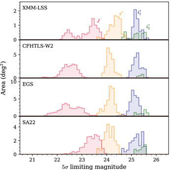
Figure 1. Histogram of the 5σ limiting magnitudes for a point-source detection of the four survey fields. Different colors represent the magnitudes in different bands, as marked in the top panel.
Download figure:
Standard image High-resolution imageTable 1. Summary of the Survey Fields
| Field | R.A. | Decl. | Area | 5σ Limiting Magnitudes (mag) / Median Seeing (arcsec) | ||||||
|---|---|---|---|---|---|---|---|---|---|---|
| (J2000) | (J2000) | (deg2) | u* |

|

|

|

|

| J | |
| XMM-LSS | 02:22:00 | −05:20:00 | 8.7 (5.9/2.8) | 25.7/0.92 | 26.1/0.86 | 25.6/0.71 | 25.3/0.74 | 25.3/0.65 | 24.5/0.71 | 23.4/0.85 |
| CFHTLS-W2 | 08:58:00 | −03:17:00 | 22.0 (20.4/1.6) | 25.6/0.88 | 26.1/0.80 | 25.5/0.73 | 25.3/0.65 | 25.5/0.61 | 24.2/0.69 | 22.6/0.90 |
| EGS | 14:18:00 | +54:30:00 | 34.4 (29.2/5.2) | 25.7/0.85 | 26.1/0.82 | 25.5/0.73 | 25.2/0.67 | 25.6/0.54 | 24.3/0.64 | 22.6/0.88 |
| SA22 | 22:11:00 | +01:50:00 | 21.1 (16.7/4.4) | 25.7/0.82 | 26.2/0.76 | 25.5/0.65 | 25.3/0.64 | 25.5/0.56 | 24.2/0.64 | 23.5/0.82 |
Note. The coordinates indicate the approximate center of each field. The numbers in parentheses are the areas observed in  and
and  bands, respectively. The limiting magnitude is given in a median value for point sources after the PSF correction for an aperture with a diameter of 2 × FWHM
 .
.
Download table as: ASCIITypeset image
2.4. Source Extraction
With SExtractor, the source detection was performed first in the  -band images, at which the Lyα
λ1216 (Lyα) emission of a z ∼ 6 quasar is expected to be located. We set the detection criteria for the SExtractor parameters to DETECT_MINAREA = 9 pixels and DETECT_THRESH = 1.3σ, allowing us to catalog only the sources with significant (≳4σ) signals in
-band images, at which the Lyα
λ1216 (Lyα) emission of a z ∼ 6 quasar is expected to be located. We set the detection criteria for the SExtractor parameters to DETECT_MINAREA = 9 pixels and DETECT_THRESH = 1.3σ, allowing us to catalog only the sources with significant (≳4σ) signals in  band. Note that this affects the photometric completeness estimation in Section 5.1.
For the  -band-detected sources, we performed aperture photometry with an aperture of 2 × FWHM
 diameter, where FWHM
 is the full width at half-maximum of point sources in
  -band images (∼0
7), by using dual-image mode in SExtractor (called forced photometry). The aperture size is determined to maximize S/N (or FLUX/FLUXERR) of the
 -band detection with comparable seeing sizes in the other bands. The aperture fluxes in each band were converted to the total fluxes by adopting the aperture correction factors derived from bright point sources in the same field, so that differences in seeing values in different bands are taken care of. Note that we use aperture instead of PSF because the PSF flux tends to be overestimated if there is no detection when doing forced photometry.
To correct for the galactic extinction (minor in our extragalactic fields; <0.05 mag), we used the extinction map of Schlafly & Finkbeiner (2011) with an assumption of RV = 3.1 (Cardelli et al. 1989).
3. Quasar Candidate Selection
3.1. Point-source Selection
Under the imaging resolution of our data, most of the high-redshift quasars with M1450 < −23.5 mag are classified as point sources (≳90%; Bowler et al. 2021). Previous studies often used the magnitude differences (e.g., PSF magnitude vs. aperture magnitude) to avoid the extended-source contamination. In this work, we adopt the SPREAD_MODEL parameter, a star−galaxy classifier in SExtractor, which denotes how the source morphology is different from the input PSF model. 15 This method offers a better performance to separate point sources from not only the extended sources but also the glitch-like spikes, compared to the previous stellarity index (CLASS_STAR) in SExtractor, especially at faint magnitudes (Annunziatella et al. 2013). The SPREAD_MODEL is defined as
where
p
is the image vector centered on the source and
W
is a weight matrix (diagonal) related to the pixel noises.  and
and  represent the point source and the galaxy model vectors at the current position, respectively. They are based on the resampled local PSF model generated with PSFEx, while the latter (
 ) is obtained by convolving an additional circular exponential model. Since the functional form is normalized by the local PSF model, sources having different PSFs in various fields can be compared to each other.
The average SPREAD_MODEL value of point sources is expected to be zero regardless of flux or S/N, but its scatter mildly increases as S/N goes lower. Therefore, we used the SPREAD_MODEL value in the  band (
 ) as a reference, considering the high S/N of z ∼ 6 quasars in
  band with Lyα emission. Figure 2 shows the
  values of the sources. There is a clear trend of point sources with
  , distinguished from the extended sources (
 ) and the glitch-like sources (
 unremarkable in this figure with their small numbers).
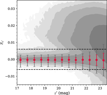
Figure 2.
 distribution of sources in the four survey fields (gray contours). The red circles denote the median
  value of the artificial stars, with the 1σ (red) and 2σ (gray) levels. The dashed lines represent our point-source selection criterion of
  .
.
Download figure:
Standard image High-resolution imageTo test how many point sources can be selected by the arbitrary  cut, we performed a simulation by adding artificial stars to the
  -band images. The artificial stars are based on the sampled stars by PSFEx in each image and scaled to match the arbitrary magnitudes that we set for the simulation. The number of the artificial stars is 100 per 0.5 mag per deg2. Then, we repeated the source extraction described in Section 2.4. The red circles in Figure 2 show the
  distribution of the artificial stars, with 1σ (68%) and 2σ (95%) levels, shown as the red and gray colors, respectively. The widening of the
  selection range decreases the number of missing point sources, but not surprisingly, the numerous contamination by extended sources also increases. With several tests, we set the criterion for the point-source selection as
  (dashed lines) to balance between them down to
  mag. With this
  criterion, 96% of point sources are recovered at
  mag, while the rate in the faintest magnitude bin (
 ) drops to 83%.
3.2. Initial Color Selection
The Lyα break of a z ∼ 6 quasar is located at λobs ∼ 8500 Å, giving a very red  color with (almost) no detection at the shorter wavelengths. On the other hand, at wavelengths longer than the Lyα emission, the quasar’s color (e.g.,
  ) tends to be blue according to the quasar continuum emission. Such colors are distinguished from those of late-type stars that are the main contaminants. Lyman break galaxies (LBGs) can also be interlopers at z ∼ 6 (Matsuoka et al. 2016, 2018c), but their expected number over our survey area is very small.
16
Hence, we ignore them in this study.
) tends to be blue according to the quasar continuum emission. Such colors are distinguished from those of late-type stars that are the main contaminants. Lyman break galaxies (LBGs) can also be interlopers at z ∼ 6 (Matsuoka et al. 2016, 2018c), but their expected number over our survey area is very small.
16
Hence, we ignore them in this study.
Figure 3 shows the color distributions of the point sources in our survey (gray contours). Following Kim et al. (2015), we set the color and magnitude selection criteria as follows:
- 1.

- 2.
- 3., ,
- 4.
- 5.J < J5σ .


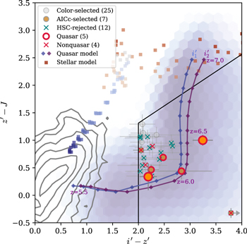
Figure 3. Color–color diagram of point sources in our survey field (gray contours). The gray circles denote the 25 color-selected candidates with errors, while the arrow indicates the lower limit in color. The seven AICc-selected candidates with wq
> 0.99 are filled with orange. The rejected candidates after the photometric cross-match with the HSC data are marked by teal crosses. The identified quasars and nonquasars are highlighted by the red open circles and crosses, respectively. The newly discovered quasars are shown as the larger symbols. The blue and purple diamonds with solid lines are the representative quasar models for  and
and  magnitudes, respectively, from z = 5.5 to 7.0 with a step of Δz = 0.1 with M1450 = −24 mag, α
P
= −1.6, and logEW = 1.542. The color distributions of the whole quasar models are shown as the underneath hexagon bins in the same colors. The late-type star model is shown as the squares, color-coded by the temperature (Teff = 3000–1000 K from blue to red colors).
magnitudes, respectively, from z = 5.5 to 7.0 with a step of Δz = 0.1 with M1450 = −24 mag, α
P
= −1.6, and logEW = 1.542. The color distributions of the whole quasar models are shown as the underneath hexagon bins in the same colors. The late-type star model is shown as the squares, color-coded by the temperature (Teff = 3000–1000 K from blue to red colors).
Download figure:
Standard image High-resolution imageNote that the magnitude with a subscript of 3σ (5σ) is the 3σ (5σ) limiting magnitude. The first two color criteria are shown as the black solid lines in Figure 3. If a source is not detected at the 3σ level (e.g.,  ), then the limiting magnitude is used for the color selection instead. Considering the point-source completeness (Section 3.1) and the i-band limiting magnitude, we set the fourth criterion in terms of
  -band magnitude. In addition, taking account of the variance in the J-band imaging depths (Figure 1), the J-band magnitude cut (the fifth criterion) is set at the 5σ detection limit of the tiling image.
Among 404 color-selected objects, there are many spurious ones with bad image quality; most of them are located in the bad pixel regions in the image of at least one filter (e.g., at the edge of the image). We automatically reject such cases, resulting in the 64 sources. Then, we performed an additional visual inspection of the remaining sources to reject obvious noncelestial objects (e.g., diffraction spikes, bad pixels, image artifacts, cosmic rays, etc.). We also cross-check the ones rejected by the above-automated process, and no object deserves to be selected through the visual inspection process. We finally have 25 candidates, which are listed in Table 2.
Table 2. IMS z ∼ 6 Quasar Candidates
| ID | R.A. (J2000) | Decl. (J2000) |

|

| J | wq |

| Spectroscopy |
|---|---|---|---|---|---|---|---|---|
| (1) | (2) | (3) | (4) | (5) | (6) | (7) | (8) | (9) |
| Color- and AICc-selected Candidates | ||||||||
| J140001+554619 a | 14:00:01.31 | +55:46:19.33 | 25.37 ± 0.15 b | 23.18 ± 0.07 | 22.85 ± 0.23 | > 0.99 | ... | Quasar |
| J140121+531434 | 14:01:21.47 | +53:14:33.51 | 24.94 ± 0.14 | 22.89 ± 0.06 | 22.07 ± 0.05 | >0.99 | ... | Nonquasar |
| J140504+542435 | 14:05:03.69 | +54:24:34.98 | >25.70 | 21.91 ± 0.03 | 22.23 ± 0.09 | >0.99 | ... | Nonquasar |
| J142952+544718 | 14:29:52.18 | +54:47:17.68 | 23.97 ± 0.07 | 21.49 ± 0.02 | 20.81 ± 0.04 | >0.99 | ... | Quasar (Willott et al. 2010) |
| J143055+531520 a | 14:30:54.67 | +53:15:20.32 | 25.44 ± 0.19 | 22.19 ± 0.05 | 21.19 ± 0.09 | >0.99 | ... | Quasar |
| J220418+011145 | 22:04:17.93 | +01:11:44.77 | 25.15 ± 0.14 | 22.90 ± 0.06 | 22.44 ± 0.07 | >0.99 | 2.68 ± 0.09 | Quasar (Kim et al. 2015) |
| J221644−001650 | 22:16:44.48 | −00:16:50.15 | 26.06 ± 0.58 | 23.23 ± 0.09 | 22.79 ± 0.12 | >0.99 | 3.34 ± 0.17 | Quasar (Matsuoka et al. 2016) |
| Color-selected Candidates | ||||||||
| J022609−054405 | 02:26:09.29 | −05:44:04.50 | 25.13 ± 0.28 b | 22.91 ± 0.05 | 22.04 ± 0.13 | 0.76 | 1.34 ± 0.04 | ... |
| J084842−012809 | 08:48:42.37 | −01:28:09.39 | 25.48 ± 0.27 | 23.44 ± 0.11 | 23.01 ± 0.21 | 0.02 | 1.19 ± 0.10 | ... |
| J085550−051346 | 08:55:50.30 | −05:13:46.02 | 25.38 ± 0.27 | 23.25 ± 0.10 | 22.69 ± 0.15 | 0.09 | ... | Nonquasar |
| J085756−050514 | 08:57:55.94 | −05:05:14.21 | 25.22 ± 0.21 | 23.16 ± 0.09 | 22.19 ± 0.09 | 0.01 | ... | ... |
| J090028−015639 | 09:00:27.73 | −01:56:39.29 | 25.89 ± 0.51 | 23.46 ± 0.13 | 22.68 ± 0.17 | <0.01 | 0.92 ± 0.10 | ... |
| J090554−052518 | 09:05:53.65 | −05:25:17.94 | 25.75 ± 0.43 | 23.48 ± 0.13 | 22.58 ± 0.18 | <0.01 | ... | Nonquasar |
| J141556+572709 | 14:15:56.03 | +57:27:08.86 | 25.14 ± 0.23 | 23.05 ± 0.07 | 21.92 ± 0.15 | <0.01 | ... | ... |
| J141752+553504 | 14:17:51.61 | +55:35:04.35 | 25.43 ± 0.24 | 23.35 ± 0.09 | 22.06 ± 0.15 | <0.01 | ... | ... |
| J143639+525452 | 14:36:39.37 | +52:54:51.71 | 25.74 ± 0.52 | 23.39 ± 0.11 | 22.29 ± 0.10 | <0.01 | ... | ... |
| J220242+014912 | 22:02:42.03 | +01:49:11.63 | 25.84 ± 0.45 | 23.43 ± 0.11 | 22.78 ± 0.15 | <0.01 | 1.20 ± 0.09 | ... |
| J220350+012638 | 22:03:50.19 | +01:26:37.69 | 25.55 ± 0.47 | 23.47 ± 0.12 | 22.92 ± 0.18 | <0.01 | 1.19 ± 0.11 | ... |
| J220431+020140 | 22:04:30.94 | +02:01:39.61 | 25.49 ± 0.48 | 23.23 ± 0.11 | 22.88 ± 0.16 | 0.02 | 1.37 ± 0.07 | ... |
| J220436+015026 | 22:04:36.49 | +01:50:26.46 | 25.24 ± 0.38 | 23.20 ± 0.10 | 22.14 ± 0.10 | <0.01 | 1.32 ± 0.04 | ... |
| J220748+035644 | 22:07:47.75 | +03:56:44.09 | 26.01 ± 0.36 b | 23.37 ± 0.13 | 22.42 ± 0.07 | <0.01 | 1.19 ± 0.11 | ... |
| J221034+024506 | 22:10:33.96 | +02:45:06.06 | 25.83 ± 0.38 b | 23.17 ± 0.09 | 22.28 ± 0.11 | 0.33 | 1.40 ± 0.07 | ... |
| J221529+003846 | 22:15:29.42 | +00:38:45.60 | 25.42 ± 0.26 | 23.38 ± 0.15 | 22.34 ± 0.07 | <0.01 | 1.31 ± 0.07 | ... |
| J221554−005155 | 22:15:54.37 | −00:51:55.22 | 25.57 ± 0.33 | 23.47 ± 0.10 | 22.79 ± 0.11 | 0.01 | 1.31 ± 0.13 | ... |
| J221725−001220 | 22:17:25.02 | −00:12:20.49 | 25.67 ± 0.34 | 23.50 ± 0.10 | 22.44 ± 0.08 | <0.01 | 1.23 ± 0.11 | ... |
Notes. Column (1): candidate name. Columns (2)–(3): sky coordinates. Columns (4)–(6): i’-,  -, and J-band magnitudes with 1σ errors. Column (7): wq
value determined from the photometric data from CFHTLS and IMS. Column (8):
-, and J-band magnitudes with 1σ errors. Column (7): wq
value determined from the photometric data from CFHTLS and IMS. Column (8):  color in PSF magnitude from the HSC-SSP PDR3 catalog (Aihara et al. 2022). Column (9): spectroscopic identification; if a quasar, the z and M1450 values are listed.
 magnitudes.
Download table as: ASCIITypeset image
3.3. AICc Selection
It has been known that the observational properties of high-redshift quasars are slightly different from those of low-redshift ones. For instance, the EW values of z ∼ 6 quasars tend to be smaller than those of low-redshift ones (Bañados et al. 2016). Previous studies, however, used the low-redshift quasar templates, which are redshifted to higher redshifts for statistical methods represented by the Bayesian approach to find high-redshift quasars (e.g., Mortlock et al. 2012; Matsuoka et al. 2016). Concerned that this issue may miss plausible candidates, we here prefer to use the models whose parameters can be easily tuned to fit the observed properties. Unlike when using observation-based templates, the complexity of the model and its potential for overfitting must be taken into account when using such models with multiple parameters. We selected models that can represent the photometric characteristics of high-redshift quasars and late-type stars well with minimal parameters, which are described below. Each model has a different number of free parameters, so we introduced an information criterion that prioritizes models for a given data set by giving an additional penalty based on the number of free parameters. This approach is known to be effective in selecting the promising high-redshift quasar candidates by comparing models of different types of celestial objects (Shin et al. 2020). Moreover, we chose this method over the well-known Bayesian approach because it takes into account the ideal characteristics and distributions of the models, unlike observation-based templates.
In this study, we introduce the Akaike information criterion (AIC; Akaike 1974), which is based on the Kullback–Leibler discrepancy (Kullback & Leibler 1951). For a model m, AIC is given by

where km
is the number of free parameters and  is the likelihood. The first term gives an additional penalty, allowing us to compute the model priority with not only
  but also km
. We have photometric information only in six bands, so a corrected version of AIC for small sample sizes (AICc; Sugiura 1978) works better than Equation (2) (Burnham & Anderson 2002), which is given by
but also km
. We have photometric information only in six bands, so a corrected version of AIC for small sample sizes (AICc; Sugiura 1978) works better than Equation (2) (Burnham & Anderson 2002), which is given by

where n is the number of filters (or photometric data) to calculate  . By comparing the AICc values from different models, we can determine which model traces the observed data more closely. Here we introduce the two models: high-redshift quasars and late-type stars.
3.3.1. High-redshift Quasar Model
We use the model of Kim et al. (2019) based on the quasar composite spectrum of Vanden Berk et al. (2001), including the IGM attenuation effect (Madau et al. 1996). It has four parameters of (z, M1450, αp , EW), where z is the redshift, M1450 is the monochromatic magnitude at 1450 Å, αp is the slope of the quasar power-law continuum, and EW is the equivalent width of the composition of Lyα and N v emissions (see Kim et al. 2019 for details). Instead of letting the parameters be free, we generated 0.1 million mock quasars that reflect the observational properties of real quasars at z ∼ 6. The redshift and the magnitude are uniformly distributed (but randomly generated) in the ranges of 5.5 < z < 7.0 and −28 < M1450 <−22. On the other hand, the other two parameters are randomly given by Gaussian distributions (mean ± standard deviation): αP = −1.6 ± 1.0 (Mazzucchelli et al. 2017) and logEW =1.542 ± 0.391 (Bañados et al. 2016). As in Kim et al. (2020), the Baldwin effect (Baldwin 1977) is also included when we generate the EW distribution, by giving the shift to the mean value using the relation between EW of Lyα and continuum flux in Dietrich et al. (2002). Although the relation is from low-redshift AGNs, we use it under the assumption of no redshift evolution in the quasar broad-line properties in rest-UV (Shen et al. 2019; Schindler et al. 2020). From these model spectra, broadband magnitudes are calculated by integrating the mock quasar spectra convolved with the filter transmission curves.
In the left panels of Figure 4, we show the color distributions of these mock quasars across the redshift. As a function of redshift, they show good agreements with the confirmed quasars not only in this work (red circles) but also from the Canada–France–Hawaii Quasar Survey (CFHQS; Willott et al. 2007, 2009, 2010; blue circles). This implies that the mock quasars emulate the real quasars at z ∼ 6 well.
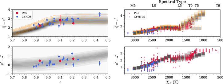
Figure 4. Left: color distributions of the high-redshift quasar models across various redshifts (gray contours). The overplotted orange contour is for the case of  -band magnitudes. The red and blue circles represent the spec-identified quasars from IMS and CFHQS, respectively, while the arrows indicate the lower limit of colors. Right: color distributions of the late-type star model as a function of Teff (gray squares). The overplotted orange open squares are for the case of
  -band magnitudes. The red and blue circles represent the observed late-type stars in the PS1 and CFHTLS photometric systems, respectively (see details in Section 3.3.2).
Download figure:
Standard image High-resolution image3.3.2. Late-type Star Model
We use the BT-Settl model (Allard et al. 2012) for late-type stars, which is publicly available on the Theoretical Spectra Web Server.
17
The model has four parameters: effective temperature (Teff), surface gravity (g), metallicity ([M/H]), and α-element enhancement (α
E
). We choose the templates in the ranges of 1000 K ≤ Teff ≤ 3000 K and 3.5 ≤ log(g) ≤ 5.5 with step sizes of ΔTeff = 100 K and  , respectively. Since the low-Teff (≤2500 K) stars have a fixed value of [M/H] = 0 and α
E
= 0, we only used the templates with those values. Note that there is no template for a star with Teff = 1000 K and
, respectively. Since the low-Teff (≤2500 K) stars have a fixed value of [M/H] = 0 and α
E
= 0, we only used the templates with those values. Note that there is no template for a star with Teff = 1000 K and  , resulting in the 20 × 5 + 4 = 104 templates. In addition, we used a normalization factor fN
as a free parameter. Like the quasar model, their magnitudes were obtained by integrating fluxes within each band.
, resulting in the 20 × 5 + 4 = 104 templates. In addition, we used a normalization factor fN
as a free parameter. Like the quasar model, their magnitudes were obtained by integrating fluxes within each band.
The right panels of Figure 4 show the color distribution of our late-type star model. For comparison, we sourced the photometry of late-type stars from the Pan-STARRS1 3π Survey (PS1) late-type star catalog (Best et al. 2018). The PS1 stellar spectral types were converted to Teff using the relations between them (Pecaut & Mamajek 2013; Bailey 2014). We also converted the PS1 magnitudes into the CFHTLS photometric system,
18
shown as the blue circles, except for the L- and T-dwarf stars without  -band photometry information. The filter systems between the two surveys are only slightly different, so we also show the colors in PS1 as blue circles in order to see the trend of such L- and T-dwarf stars. As in this figure, our late-type star models are broadly consistent with the real stars.
3.3.3. SED Fitting and AICc-based Criterion
We performed the fitting for the spectral energy distributions (SEDs) of the 25 color-selected candidates in Section 3.2 with the above high-redshift quasar and late-type star models. As in Kim et al. (2019), for a model m, we find the best-fit solution that minimizes the modified χ2 statistic:

This statistic is to consider both detected and undetected cases (subscripts of d and u, respectively). The first term is a sum of the typical χ2 statistic for the detected fluxes, given as
where Fo,d is the observed flux in the dth band, Fm,d is the model flux, and σo,d is the uncertainty of Fo,d . On the other hand, the second term gives an additional penalty for the cases of upper limit, defined by Sawicki (2012):
where  is the upper limit of flux in the uth band, while Fo,u
, Fm,u
, and σo,u
are the observed flux, model flux, and sensitivity in the same band, respectively. Parameter
is the upper limit of flux in the uth band, while Fo,u
, Fm,u
, and σo,u
are the observed flux, model flux, and sensitivity in the same band, respectively. Parameter  is the error function of
  , for the numerical calculation.
We calculate  (
( ) for the SEDs of the color-selected candidates. For example, if a candidate is detected in the
  ,
,  , and J bands, we calculate
  for these bands and
  for the other bands. The best-fit quasar and star models, which minimize
  values, are shown as the blue and orange lines, respectively, in Figure 5.
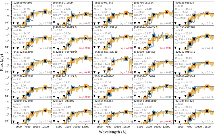
Figure 5. SED-fitting results for the color-selected candidates. The black circles and downward-pointing triangles are the photometric data points and their upper limits, respectively. The blue and orange lines are the best-fit high-redshift quasar and late-type star models, respectively, while the open squares in the same colors represent fluxes in each band. The key best-fit parameters of each candidate are marked in each panel. The AICc-selected candidates with wq > 0.99 are highlighted with star symbols.
Download figure:
Standard image High-resolution imageUsing Equations (2) and (3), we compute AICcq and AICcs , where the subscripts q and s denote the high-redshift quasar and late-type star models, respectively. Since our purpose is to determine whether a candidate is more likely to be a quasar or not, we only compare the best-fit cases from the two models. To prioritize the models, we introduce the weights of AICc (Burnham & Anderson 2002), given by
where

and  is the minimum of the AICc values (min[AICcq
, AICcs
]). This weight can be interpreted as the probability that the given model is the best one. For the color-selected candidates, we listed their wq
values in Table 2.
is the minimum of the AICc values (min[AICcq
, AICcs
]). This weight can be interpreted as the probability that the given model is the best one. For the color-selected candidates, we listed their wq
values in Table 2.
We set a very strict criterion of wq > 0.99. This corresponds to the fraction of the weights of wq /ws ≳ 100, meaning that the high-redshift quasar model is ≳100 times more likely to be the best model than the late-type star model (Burnham & Anderson 2002). This choice is because our late-type star model has a very small scatter in colors, compared to the observed ones, as shown in Figure 4. There are seven candidates satisfying this criterion, shown as the orange filled circles in Figure 3.
3.4. Photometric Cross-check with HSC
Several parts of our survey area overlap with the area of the Wide Survey of HSC-SSP. On average, the optical images from the HSC-SSP Public Data Release 3 (PDR3; Aihara et al. 2022) are ≳1 mag deeper than those from CFHTLS. Therefore, we expect more accurate photometry for the overlapping targets.
We found that 14 of the color-selected candidates are in the overlapping area, by matching our candidates to the sources in the HSC-SSP PDR3 catalog. We adopted the HSC-SSP PDR3's PSF magnitudes in the  and
and  bands, listed in Table 2 in the
  form. Note that the filter systems of CFHTLS and HSC are slightly different from each other, especially in the
  and
and  bands. While their central wavelengths are similar to each other (8815 and 8908 Å, respectively), the former has a broader bandwidth of 1040 Å than the latter, which has a bandwidth of 781 Å. This makes different color trends of quasars on the color–color diagram, as shown in Figure 6. For our quasar model, the
  color (yellow diamonds) is redder at z ∼ 6 and becomes bluer at z > 6.5 than
  (blue and purple diamonds).
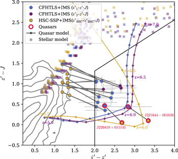
Figure 6. Color–color diagram of the 14 HSC-overlapped candidates (filled circles), similar to Figure 3. The blue, purple, and yellow colors represent the combinations of  –
– –J,
–J,  –
– –J, and
  –
– –J, respectively. The diamonds with lines are the representative high-redshift quasar models, while the late-type star models are shown as squares with the given colors regardless of the temperature. The gray lines indicate that the connected circles are the same candidates. The spec-identified quasars are highlighted by red circles with their IDs.
Download figure:
Standard image High-resolution imageMost of the HSC-overlapped candidates (12/14) have bluer colors of  . If we use
  and
and  instead of
  and
and  , respectively, the 12 candidates move toward the stellar locus in the color–color diagram (yellow circles), meaning that they are unlikely to be z ∼ 6 quasars or even galaxies at that redshift (Harikane et al. 2021). It is remarkable that all of them are also rejected by our AICc selection using the CFHTLS optical photometry. On the other hand, the colors of the other two candidates, highlighted by red circles, are still likely to be those of the high-redshift quasar models even if using the HSC colors. We note that they satisfy our AICc selection criterion and were also identified as high-redshift quasars by spectroscopy (Kim et al. 2015; Matsuoka et al. 2016). This demonstrates that our AICc selection, even under shallower imaging data, is an effective method to exclude nonquasar objects.
On the contrary, there may be objects that have red  colors in HSC but not so in our data. From the HSC-SSP PDR3 catalog, we select point sources with
  using the selection criteria given in Equation (1) of Matsuoka et al. (2018c), which are also detected in CFHTLS
  -band images. There are seven isolated point sources at
  mag, while the brightest one among them has
  in our data. This is because of its brighter
  -band magnitude in IMS (
 vs.
vs.  ), while there is no significant difference in
  -band magnitudes (
 mag vs.
  ). We note that this object is close to the edge of the CFHTLS image. This implies that 14% (1/7) of red objects could be missed in our imaging data, especially for
  mag objects.
4. Spectroscopic Identification
In previous studies, three of our candidates were already identified as z ∼ 6 quasars: J142952+544718 (Willott et al. 2010), J220418+011145 (Kim et al. 2015, 2018), and J221644−001650 (Matsuoka et al. 2016). For the remaining targets, we additionally obtained their spectra with the Palomar 200-inch and Gemini telescopes.
4.1. P200/DBSP Observation
We carried out spectroscopic observations of the other four AICc-selected candidates with the Double Spectrograph(DBSP) on the Palomar Hale 200-inch telescope (P200) on 2021 July 13 (PID:CTAP2021-A0032), under the seeing condition of ∼15. We used the grating of 316 lines mm–1 with a 1
5-width slit, giving the resolution of R = 956. To avoid the duplication of the zeroth-order spectrum, the D55 dichroic filter (λobs > 5500 Å) was used. The total exposure times are 3600 s for fainter ones (J140001+554619 and J140121+531434) and 1200 s for the other brighter ones (J140504+542435 and J143055+531520).
For data reduction, we used the PypeIt Python package
19
(Prochaska et al. 2020a, 2020b). This is an open-source pipeline for the selected instruments, which automatically performs the bias subtraction, flat-fielding, skyline subtractions, and wavelength calibrations (with HeNeAr arc lines). Considering the faintness of our target, we manually extracted fluxes within an optimal aperture with a fixed FWHM that matches the seeing size (15). The flux calibration was also done by PypeIt with the standard star, Feige 110. In addition, we scaled the spectra to match with their
 -band photometry to compensate for the flux loss by sky fluctuation, as was done in Kim et al. (2019) and Kim et al. (2020). By convolving the
  -band transmission curve with the three spectra (except for J140121+531434 without detection), we obtained scaling factors of 1.54–1.78. We applied the average scaling factor of 1.69 to all the DBSP spectra. Note that the limited wavelength coverage of our spectra up to ∼10000 Å may affect the scaling factor. Finally, we binned the spectra in the spectral direction with resolutions of R = 956 and 300 by using the inverse-variance weighting method (e.g., Kim et al. 2018).
We show the DBSP spectra of the four candidates in Figure 7. Except for the faintest, J140121+531434, their spectra are marginally detected with low S/N of 2–3. J140001+554619 and J143055+531520 show clear breaks at ∼8400 and 8850 Å, respectively. Such breaks are more clearly visible if we maximize the S/N by binning the data to a low resolution of R = 300 (right columns in Figure 7). We provide more detailed individual notes for these targets in Section 4.3.

Figure 7. P200 optical spectra of four quasar candidates, after binning with resolutions of R = 956 (instrumental setup; left) and 300 (right). The blue lines represent the flux uncertainties in the 1σ level. The red lines on the spectra of J140001+554619 and J143055+531520 are their best-fit high-redshift quasar models, of which emission-line locations are marked as the red vertical ticks (Lyβ
λ1025, Lyα
λ1216, N v
λ1240, O i
λ1304, and C ii
λ1335 from left to right). The purple squares show the  -band fluxes with its bandwidth. The bottom panels show the normalized skylines. Note that the y-axis of the 2D spectra is given in units of arcsec.
Download figure:
Standard image High-resolution imageAs mentioned above, J140121+531434 is not detected, even though its  -band magnitude is brighter than J140001+554619. For a high-redshift quasar, the peak of Lyα flux in its spectrum is expected to be brighter than broadband photometry (
 band; purple squares), which is dominantly determined by continuum emission, but this object shows no remarkable feature. On the other hand, the spectrum of J140504+542435 has continuum emissions without any remarkable emission lines or breaks. Therefore, we concluded that J140121+531434 and J140504+542435 are not high-redshift quasars but interlopers like late-type stars or faint galaxies.
4.2. Gemini/GMOS Observation
We obtained the spectra of J085550−051346 and J090554−052518 with the Gemini Multi-Object Spectrograph (GMOS; Hook et al. 2004) on the Gemini-South 8 m Telescope on 2020 February 24 (PID: GS-2020A-Q-219). Note that these observations preceded the AICc selection. The seeing condition was ∼07. Since the targets are very faint, we optimized the observing configurations to maximize S/N. The choice of an R150_G5326 grating with a slit width of 1
0 gives a low resolution of R ∼ 315, and we set the 4 × 4 binning in the spatial/spectral directions. The nod-and-shuffle mode was used to subtract skylines accurately. The total exposure times are 2904 and 3388 s for J085550−051346 and J090554−052518, respectively.
We followed the general reduction process for the GMOS spectra using the Gemini IRAF package: (1) bias subtraction, (2) flat-fielding, (3) skyline subtraction, (4) wavelength calibration with CuAr arc lines, and (5) flux calibration with a standard star LTT2415. Note that for the extraction process we used a fixed aperture whose size is consistent with the seeing size of ∼07. Like DBSP spectra, the GMOS spectra were scaled to match with
 -band magnitudes, by a factor of 2.25 on average. Such a large scaling factor might be due to the reported problem on the coefficient of thermal expansion during our observing run.
20
We also binned the spectra along the spectral direction to match the instrument resolution of R = 315.
-band magnitudes, by a factor of 2.25 on average. Such a large scaling factor might be due to the reported problem on the coefficient of thermal expansion during our observing run.
20
We also binned the spectra along the spectral direction to match the instrument resolution of R = 315.
The two spectra are shown in Figure 8. Both show clear continua but without any remarkable emission lines or Lyα break, suggesting that they are not high-redshift quasars. We here emphasize that they dissatisfy the AICc criterion, supporting the feasibility of our approach.
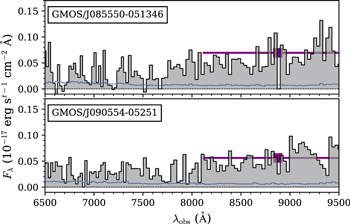
Figure 8. GMOS optical spectra of two quasar candidates, dissatisfying the AICc criterion. The symbols are the same as in Figure 7.
Download figure:
Standard image High-resolution image4.3. Spectral Properties of New Quasars
For J140001+554619 and J143055+531520, which are likely to be high-redshift quasars with clear breaks on their spectra, we measured their z and M1450 by finding the best-fit models among our mock quasars in Section 3.3.1. We calculated the reduced chi-square values ( ) between their spectra and our mock quasar spectra. The wavelength range for the spectral fitting was set as 6500 Å < λobs < 9500 Å. We chose the best-fit models of J140001+554619 and J143055+531520 with the minimum
  values of
  and 1.09, respectively, which are shown as the red lines in Figure 7. The best-fit parameters are listed in Table 3, along with the results from the photometric data (Section 3.3.3). We also list the measurements of the three previously known quasars at z ∼ 6 (Willott et al. 2010; Kim et al. 2015; Matsuoka et al. 2016; Kim et al. 2018).
Table 3. Best-fit Parameters of IMS z ∼ 6 Quasars
| ID | Spectroscopy | Photometry | Spectral Reference | ||||||
|---|---|---|---|---|---|---|---|---|---|
| z | M1450 | αP | logEW | z | M1450 | αP | logEW | ||
| J140001+554619 | 5.85 | −23.25 | −1.49 | 1.54 | 5.87 | −23.54 | −1.29 | 1.16 | This work |
| J143055+531520 | 6.29 | −25.45 | −0.80 | 1.56 | 6.28 | −25.12 | −0.31 | 1.73 | This work |
| J142952+544718 | 6.21 | −25.85 | ... | ... | 6.00 | −25.44 | −0.44 | 1.44 | Willott et al. (2010) |
| J220418+011145 | 5.93 | −23.99 | ... | ... | 5.96 | −23.82 | −0.78 | 1.62 | Kim et al. (2015, 2018) |
| J221644−001650 | 6.10 | −23.56 | ... | ... | 6.13 | −23.72 | −1.58 | 1.61 | Matsuoka et al. (2016) |
Note. This table provides the parameters of the high-redshift quasar models (Section 3.3.1), which are best-fitted for the spectroscopy and photometry of the IMS z ∼ 6 quasars, respectively.
Download table as: ASCIITypeset image
The clear break of J140001+554619 at ∼8400 Å is consistent with the z = 5.85 quasar model. Interestingly, some peaky detections on the spectrum are also in line with the locations of quasars’ high-ionization emission lines: O i λ1304 and C ii λ1335 (red vertical markers in Figure 7). The existence of the probable emission lines may provide additional evidence supporting its nature as a high-redshift quasar. However, since the S/Ns of the two peaky detections are as low as 2.7 and 1.9, respectively, we still have doubts about their reliability. LBGs would have a clear Lyman break on their spectra too, so it is difficult to confidently say that J140001+554619 is not a z ∼ 6 LBG, although we have ignored them in our selection process. Further observations are needed to identify the high-ionizing emission lines, which can be a crucial criterion for determining whether this object is a quasar or LBG. In the following sections, we assume that J140001+554619 is a high-redshift quasar, but we here caution that our estimates could be overestimated if this object is actually an LBG.
In the case of J143055+531520, there is a clear Lyα break with a plausible N v λ1240 emission line (S/N ∼ 7) calculated from peaky emissions at 9010–9072 Å on the R = 300 spectrum), which is consistent with the z = 6.29 quasar model. With little chance of finding LBGs as bright as this target (M1450 = −25.12 mag; inferred from the LBG LF of Harikane et al. 2021), we conclude that J143055+531520 is a high-redshift quasar.
The photometric redshifts (zphot) of the five spectroscopically identified quasars are well in line with the spectroscopic redshifts (zspec); the standard deviation of δ
z = (zphot −zspec)/(1 + zspec) is only 0.013. This is much smaller than the value for z ∼ 5 quasars using the same model (0.043; Kim et al. 2019), which might be due to the stronger IGM attenuation at higher redshifts, despite the small number statistics. The DBSP spectra with low S/N of 2–3 and limited wavelength ranges of λobs < 9500 Å give a degeneracy of M1450, αp
, and EW in the fitting at λobs ≳ 9000 Å. Meanwhile, our SED fitting for photometry includes  - and J-band magnitudes, enabling us to estimate M1450 better. Therefore, we use their magnitudes from photometry instead of those from spectra in the following analysis.
5. Quasar Space Density
5.1. Survey Completeness
As mentioned in Section 2.3, the imaging depths of our survey are not uniform (Figure 1). Therefore, we calculated the completeness for every 1 arcmin2 area (hereafter “patch”), given as a function of z and M1450: fX,p (z, M1450), where X is the type of completeness and p is the index of each patch. We used bin sizes of dz = 0.05 and dM1450 = 0.2 mag, including more than 100 mock quasars (Section 3.3.1) in each bin.
5.1.1. Detection and Point-source Selection Completeness
We first consider the photometric completeness related to the source detection. We used the artificial stars from a simulation described in Section 3.1 to test how many of them can be recovered with our images and methods along with the magnitude (Section 2.4). The resultant completeness is parameterized by the equation of Fleming et al. (1995):
where α50 is the slope of the function at the 50% completeness magnitude ( ). The results for each CFHTLS tile are shown as the red lines in Figure 9, while the median values are highlighted by the thick solid line.
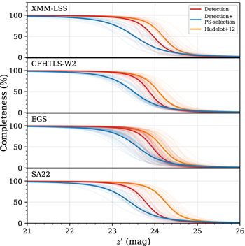
Figure 9. Point-source detection completeness of our  -band images in the four survey fields. The red and blue lines are the results of including our detection criteria and detection+point-source selection criteria, respectively. The orange lines are the completeness function by Hudelot et al. (2012) that used more lenient detection criteria. The translucent lines denote the completeness of each CFHTLS tile, while the median values are highlighted by the thick solid lines.
Download figure:
Standard image High-resolution imageFor comparison, we also parameterized the photometric completeness of Hudelot et al. (2012) with Equation (9), shown as the orange lines. Note that the functions were shifted in the magnitude direction by following our new zp measurements. Our results show lower  (≲24 mag) than Hudelot et al. (2012). This is because of our choice of SExtractor parameters for searching high-S/N sources: DETECT_MINAREA = 9 and DETECT_THRESH = 1.3. These are more stringent than DETECT_MINAREA = 3 and DETECT_THRESH = 1.0 used by Hudelot et al. (2012). If we use these values instead, our simulation gives consistent results with Hudelot et al. (2012). But we point out that there is only a negligible difference in detection rate (<1%) between ours and that of Hudelot et al. (2012) at
  mag.
mag.
In addition to the detection completeness, we consider the point-source selection described in Section 3.1. Using Equation (9), we also fitted the binned completeness for the detected sources satisfying our point-source selection criterion. The results are shown as the blue lines in Figure 9, which have  mag on average, which is naturally lower than those of the detection completeness limits. This means that our magnitude cut of
  mag is very marginal. Using the mock quasar sample described in Section 3.3.1, we converted the completeness for a given patch to a function of z and M1450: fD,p
(z, M1450).
mag is very marginal. Using the mock quasar sample described in Section 3.3.1, we converted the completeness for a given patch to a function of z and M1450: fD,p
(z, M1450).
5.1.2. Color Selection Completeness
Our initial selection is based on the colors, so we calculate the quasar selection efficiency of our color selection criteria described in Section 3.2. We gave random Gaussian noises to the magnitudes of the mock quasars according to the imaging depths at a given patch. Then, the fraction of quasars satisfying the criteria in each (z, M1450) bin was calculated, resulting in the color selection completeness of fC,p
(z, M1450). Note that the difference between the  - and
- and  -band images is also considered.
5.1.3. AICc Selection Completeness
We considered the application of the AICc selection for the final candidates. The fraction of the mock quasars satisfying wq > 0.99 was calculated patch by patch as in Section 5.1.2. Since the mock quasars have no error information in their magnitudes, we gave appropriate magnitude errors according to their magnitudes and imaging depths in each patch. The resultant completeness, fA,p (z, M1450), shows 90% down to M1450∼ −23.5 mag, meaning that the AICc selection does not reduce the total selection completeness significantly at the magnitude ranges of interest.
5.1.4. Total Selection Completeness
At a given patch, the total selection completeness is calculated by multiplying the above completeness functions because they are independent of each other: fp
= fD,p
× fC,p
× fA,p
. Then, we combined fp
in each field to get the average completeness: ![${F}_{\mathrm{field}}(z,{M}_{1450})=\left[{\sum }_{\mathrm{field}}{f}_{p}(z,{M}_{1450})\right]/{N}_{\mathrm{field}}$](https://content.cld.iop.org/journals/1538-3881/164/3/114/revision1/ajac81c8ieqn142.gif) , where Nfield is the total number of the patches in the field. Figure 10 shows the resultant completeness Ffield(z, M1450) of each field. As can be inferred from the quasar track in Figure 3, the difference between the
, where Nfield is the total number of the patches in the field. Figure 10 shows the resultant completeness Ffield(z, M1450) of each field. As can be inferred from the quasar track in Figure 3, the difference between the  - and
- and  -band filters is reflected in the results; the usage of the
  -band filter can catch more quasars at z < 5.9. The two brighter quasars are in the parameter space where the completeness is ∼1, while the remaining three fainter ones have completeness values of 0.1–0.3. But this is because they are found in the survey area of the SA22 and EGS fields, where deeper J-band images are available. Indeed, fp
(z, M1450) for the three quasars is 0.2–0.5, which rather deserves to be selected. We also calculated the total completeness (
-band filter can catch more quasars at z < 5.9. The two brighter quasars are in the parameter space where the completeness is ∼1, while the remaining three fainter ones have completeness values of 0.1–0.3. But this is because they are found in the survey area of the SA22 and EGS fields, where deeper J-band images are available. Indeed, fp
(z, M1450) for the three quasars is 0.2–0.5, which rather deserves to be selected. We also calculated the total completeness (![$F(z,{M}_{1450})=\left[\sum {f}_{p}(z,{M}_{1450})\right]/{N}_{p}$](https://content.cld.iop.org/journals/1538-3881/164/3/114/revision1/ajac81c8ieqn146.gif) ), shown in Figure 11.
), shown in Figure 11.
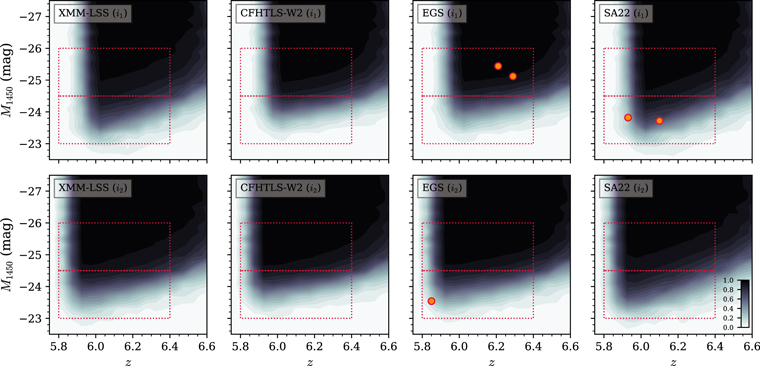
Figure 10. Selection completeness in each field as a function of z and M1450, Ffield(z, M1450), divided into the cases of  (top row) and
  (bottom row) bands. The color bar shows the completeness level. The orange circles are the spec-identified quasars, listed in Table 3. The red boxes indicate the two bins for estimating space density.
Download figure:
Standard image High-resolution image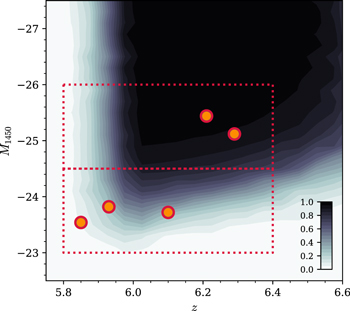
Figure 11. Total selection completeness as a function of z and M1450. The symbols are the same as in Figure 10. The red boxes indicate the two bins for estimating space density.
Download figure:
Standard image High-resolution image5.2. Binned Space Density
As listed in Table 3, we have five z ∼ 6 quasars identified by spectroscopy within the IMS survey area, including the two new quasars in this work. Their z–M1450 distributions are shown as the orange filled circles in Figure 10. With this complete sample of z ∼ 6 quasars, we calculate the binned space density using the 1/Va method of Avni & Bahcall (1980), where Va is the specific comoving volume. For given bin sizes of ΔM1450 and Δz, Va can be calculated as

where dVc
/dz is the comoving element of our survey area. Then, we calculate the binned space density (Φbin) and its error ( ) as follows:
and
where Nbin is the number of objects in the given bin. This method critically depends on the choice of the bin. Considering the small number of our sample, we set a single redshift bin of 5.8 < z < 6.4. The average redshift of our sample is z = 6.08. Meanwhile, we took two large M1450 bins: −26.0 ≤ M1450 < −24.5 and −24.5 ≤ M1450 < −23.0 (red boxes in Figures 10 and 11). Such large bins in M1450 were chosen because our sample is small but complete. There are two and three quasars in each bin, and their average magnitudes are M1450 = −25.28 and −23.69 mag, respectively. The resultant Φbin values are listed in Table 4 (top two rows). We note that the average redshifts of the two bins are z = 6.25 and 5.97, respectively. The discrepant redshift values reflect the shape of the completeness function and the larger volume available for higher redshifts for the brighter sample. We consider both of the points representing the z ∼ 6 quasar space density considering the small number statistics and the small redshift difference.
Table 4. Binned Space Density of IMS z ∼ 6 Quasars
| Field | M1450 | Δ M1450 | Nbin | Va | Φbin |
|---|---|---|---|---|---|
| (mag) | (mag) | (Gpc3) | (Gpc−3 mag−1) | ||
| Total | −25.28 | 1.5 | 2 | 0.31 | 4.27 ± 3.02 |
| −23.69 | 1.5 | 3 | 0.14 | 13.8 ± 8.0 | |
EGS ( ) ) | −25.28 | 1.5 | 2 | 0.10 | 13.0 ± 9.2 |
EGS ( ) ) | −23.54 | 1.5 | 1 | 0.01 | 61.9 ± 61.9 |
SA22 ( ) ) | −23.77 | 1.5 | 2 | 0.03 | 39.3 ± 27.8 |
Download table as: ASCIITypeset image
Despite the small number of our sample, we additionally calculated the binned space densities in the three survey fields where the quasars are identified: EGS ( ), EGS (
 ), and SA22(
 ). The results are given in the bottom three rows of Table 4, which are higher than the one for the total survey area. We discuss this in the following section.
6. Discussion
In Figure 12, we compare our results with those from the literature (Willott et al. 2010; Jiang et al. 2016; Matsuoka et al. 2018c; Giallongo et al. 2019; Grazian et al. 2020), after the correction for the cosmological parameters. For the results from faint X-ray AGNs at z ∼ 5.5 (Parsa et al. 2018; Giallongo et al. 2019; Grazian et al. 2020), we adopted the density shift to z = 6 using the density scaling factor of 10−0.72Δz at z = 5–6 (Jiang et al. 2016). Note that Matsuoka et al. (2018c) derived their space densities including the samples of Willott et al. (2010) and Jiang et al. (2016). We also show the Matsuoka et al. (2018c) LF in a double-power-law function (blue solid line). Our space densities from the total survey area (red circles) are broadly consistent with those from the previous large surveys for UV quasars (Willott et al. 2010; Jiang et al. 2016; Matsuoka et al. 2018c), despite large errors with the small number statistics. In the intermediate magnitude range of −24 < M1450 < −22 in question, our result shows the suppressed space density in line with the recent quasar LF of Matsuoka et al. (2018c). Therefore, our result reinforces the suggestion that quasars are not the main contributor to the reionizing process at z ∼ 6 (e.g., Ricci et al. 2017; Dayal et al. 2020; Jiang et al. 2022), disfavoring the AGN-dominant scenario (e.g., Giallongo et al. 2015; Madau & Haardt 2015).
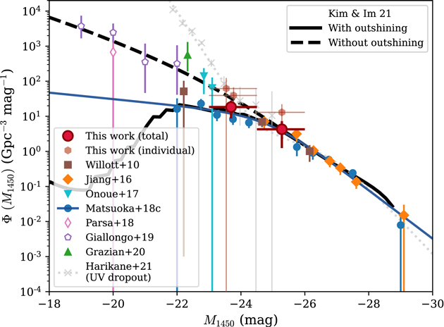
Figure 12. Quasar space densities at z ∼ 6. The red circles represent our results from the total survey area, while the red hexagons are from the three individual fields where high-redshift quasars are identified. The other symbols represent those in the literature (Willott et al. 2010; Jiang et al. 2016; Onoue et al. 2017; Matsuoka et al. 2018c; Parsa et al. 2018; Giallongo et al. 2019; Grazian et al. 2020). The filled (open) symbols are from the surveys based on rest-UV photometry (X-ray detection). The blue line shows the parametric LF of quasar (Matsuoka et al. 2018c). The black solid (dashed) line represents the quasar LF model with (without) the outshining effect (Kim & Im 2021). The parametric LF of UV dropout objects (or AGN+galaxy; Harikane et al. 2021) is auxiliary, shown as the gray crosses with dotted line.
Download figure:
Standard image High-resolution imageOur main result, however, is somewhat different from the space densities of Onoue et al. (2017) and Grazian et al. (2020), both from the AGNs identified by rest-UV spectroscopy, favoring a continuous increase in space density from bright to faint AGN populations. But we here point out that the fundamental limitation of these two studies is their small survey areas (6.5 and 0.15 deg2, respectively) and corresponding small Va
, which could result in the overestimated space densities. For instance, we show the space densities from our three individual fields where high-redshift quasars are discovered (red hexagons): EGS ( ), EGS (
 ), and SA22 (
 ). As in the two studies, the results are from one or two quasars in the small survey area (29.2, 5.2, and 16.7 deg2), which may give higher space densities than those from our total survey area.
Grazian et al. (2020) suggest that their higher space density is due to the stringent color selection criteria of the other studies (e.g.,  in Matsuoka et al. 2018c), while the two quasars they used (GDN 3333 and GDS 3073) have moderate
  -matched colors: 0.12 and 0.69, respectively. But the two quasars are at z = 5.2 and 5.6, respectively, so it would be better to check their
  colors instead to see whether they can be selected by the traditional color selection. From the CANDELS catalogs (Guo et al. 2013; Barro et al. 2019), we found that their (
 )-matched colors
21
are 2.11 and 3.03, respectively. These are red enough to be selected as a quasar candidate with a color selection (e.g.,
)-matched colors
21
are 2.11 and 3.03, respectively. These are red enough to be selected as a quasar candidate with a color selection (e.g.,  for z > 5 quasars; Kim et al. 2020), so the strict color selection cannot solely explain the discrepancy clearly.
From a different point of view, such high densities can be explained with the recent quasar LF model by Kim & Im (2021). This model is based on the empirical scaling relations of dark matter halos, galaxies, and black holes, while the key idea is that an AGN outshining its host galaxy can be observed as a point-source-like quasar. In Figure 12, we show the model with/without the outshining effect as the black solid/dashed lines, respectively. Note that we show the models including the gravitational lensing effect of Pacucci & Loeb (2020). These models suggest that the discrepancy in space density between rest-UV quasars (e.g., Matsuoka et al. 2018c; this work) and faint X-ray AGNs from some previous works (e.g., Giallongo et al. 2019) can be explained if a large fraction of AGNs become dimmer in UV than its host galaxy.
The high space densities of Onoue et al. (2017) and Grazian et al. (2020) are in line with the model without the outshining effect. It is worth noting that the AGNs used in these studies have distinct properties from typical bright quasars. For example, ELAIS 109100446, one of the two AGNs in Onoue et al. (2017), has only a narrow Lyα line without any other emission lines on its rest-UV spectrum, which indicates that it could be an Lyα emitter galaxy (Kashikawa et al. 2015). GDN 3333 in Grazian et al. (2020) shows similar features on its spectrum (Barger et al. 2002), while it is classified as an AGN with strong X-ray detection (Alexander et al. 2003; Giallongo et al. 2019). GDS 3073, another quasar in Grazian et al. (2020), is likely a Seyfert galaxy based on the morphological decomposition, while it has no X-ray detection. Taken together, their observational properties appear to be a mixture of AGNs and UV-bright galaxies, so their presence is consistent with the framework of Kim & Im (2021).
It has recently been claimed that the M1450 boundary between AGN and star-forming galaxy (represented by an LBG) is blurred, i.e., the AGN fraction of UV sources changes smoothly at −24 ≲ M1450 ≲ −22 (Adams et al. 2020; Bowler et al. 2021; Harikane et al. 2021). In Figure 12, we show the LF of UV dropout objects at z ∼ 6 (gray crosses; Harikane et al. 2021). Compared to their best-fit result (gray dotted line), our faint bin gives an AGN fraction of ∼30% at M1450 = −23.7 mag, which is lower than those at lower redshifts (e.g., ∼80% at z ∼ 4; Bowler et al. 2021). This is naturally explained by the more dramatic changes in AGN numbers between 4 ≲ z ≲ 7 (Matsuoka et al. 2018c; Akiyama et al. 2018; Wang et al. 2019; Kim et al. 2020; Niida et al. 2020) than galaxy numbers in UV (Song et al. 2016; Ono et al. 2018; Behroozi et al. 2019; Harikane et al. 2021).
7. Summary
In this work, we present the final result of the IMS z ∼ 6 quasar survey. Over the 86 deg2 sky area of CFHTLS-IMS overlap regions, 25 candidates satisfying the traditional color selection criteria were picked up. We additionally applied the AICc selection based on the SED fitting, resulting in the seven credible candidates. While three of them are known z ∼ 6 quasars, our follow-up spectroscopy for the remaining candidates leads us to discover two new z ∼ 6 quasars. Such a high success rate (5/7) proves that our new approach with the AICc method allows us to find plausible candidates efficiently. With the complete sample of five quasars, we estimated the quasar space density down to M1450 = −23.5 mag at z ∼ 6: Φbin = 4.3 and 14 Gpc−3 mag−1 at M1450 = −25.3 and −23.7 mag, respectively. These low numbers are consistent with the recent estimates from other large surveys, which endorses the minor role of quasars in the ionizing process in the reionization era.
We thank Marios Karouzos and Jueun Hong for their valuable contribution to IMS. We also thank the anonymous referee for suggestions that improved the quality of the draft. This work was supported by the National Key R&D Program of China (2016YFA0400703) and the National Research Foundation of Korea (NRF) grant funded by the Korean government (MSIT; Nos. 2020R1A2C3011091, 2021M3F7A1084525). Y.K. acknowledges the support from the China Postdoc Science General (2020M670022) and Special (2020T130018) Grants funded by the China Postdoctoral Science Foundation and was supported by the National Research Foundation of Korea (NRF) grant funded by the Korean government (MSIT; No. 2021R1C1C2091550). M.K. was supported by the National Research Foundation of Korea (NRF; No. 2022R1A4A3031306). S.S. acknowledges support by the Basic Science Research Program through the National Research Program through the National Research Foundation of Korea (NRF) funded by the Ministry of Education (No. 2020R1A6A3A13069198). M.H. acknowledges the support from the Korea Astronomy and Space Science Institute grant funded by the Korean government (MSIT; No. 2022183005). B.L. acknowledges the support from the Korea Astronomy and Space Science Institute grant funded by the Korean government (MSIT; project No. 2022-1-840-05). H.D.J. was supported by the National Research Foundation of Korea (NRF) grant 2022R1C1C2013543 funded by the Ministry of Science and ICT (MSIT) of Korea. D.K. was supported by the National Research Foundation of Korea (NRF) grant funded by the Korean government (MSIT; Nos. 2021R1C1C1013580 and 2022R1A4A3031306). S.L. acknowledges support from a National Research Foundation of Korea (NRF) grant (2020R1I1A1A01060310) funded by the Korean government (MIST). Y.C.T. acknowledges the support from the Basic Science Research Program through the National Research Foundation of Korea (NRF) funded by the Ministry of Education (No. 2021R1A6A3A14044070).
This research uses data obtained through the Telescope Access Program (TAP; PID: CTAP2020-B0043, CTAP2021-A0032). The data from the former program are not included in this paper because of their condition. Observations obtained with the Hale Telescope at Palomar Observatory were obtained as part of an agreement between the National Astronomical Observations, Chinese Academy of Sciences, and the California Institute of Technology.
This work was supported by K-GMT Science Program (PID: GS-2020A-Q-219) of the Korean Astronomy and Space Science Institute (KASI). Based on observations obtained at the international Gemini Observatory, a program of NSF’s NOIRLab, which is managed by the Association of Universities for Research in Astronomy (AURA) under a cooperative agreement with the National Science Foundation on behalf of the Gemini Observatory partnership: the National Science Foundation (United States), National Research Council (Canada), Agencia Nacional de Investigación y Desarrollo (Chile), Ministerio de Ciencia, Tecnología e Innovación (Argentina), Ministério da Ciência, Tecnologia, Inovações e Comunicações (Brazil), and Korea Astronomy and Space Science Institute (Republic of Korea).
The Pan-STARRS1 Surveys (PS1) and the PS1 public science archive have been made possible through contributions by the Institute for Astronomy, the University of Hawaii, the Pan-STARRS Project Office, the Max-Planck Society and its participating institutes, the Max Planck Institute for Astronomy, Heidelberg and the Max Planck Institute for Extraterrestrial Physics, Garching, Johns Hopkins University, Durham University, the University of Edinburgh, the Queen’s University Belfast, the Harvard-Smithsonian Center for Astrophysics, the Las Cumbres Observatory Global Telescope Network Incorporated, the National Central University of Taiwan, the Space Telescope Science Institute, the National Aeronautics and Space Administration under grant No. NNX08AR22G issued through the Planetary Science Division of the NASA Science Mission Directorate, the National Science Foundation grant No. AST-1238877, the University of Maryland, Eotvos Lorand University (ELTE), the Los Alamos National Laboratory, and the Gordon and Betty Moore Foundation.
This publication makes use of data products from the Two Micron All Sky Survey, which is a joint project of the University of Massachusetts and the Infrared Processing and Analysis Center/California Institute of Technology, funded by the National Aeronautics and Space Administration and the National Science Foundation.
Facilities: CFHT (MegaCam) - , Hale (DBSP) - , Gemini:South (GMOS-S) - , UKIRT (WFCAM). -
Software: PSFEx (Bertin 2011), PypeIt (Prochaska et al. 2020a, 2020b), SExtractor (Bertin & Arnouts 1996), SWarp (Bertin 2010).
Appendix: Quasar Candidate Selection without J-band Detection
The fifth criterion of our initial color selection (J < J5σ in Section 3.2) allows us to select only the sources with significant J-band detections. But we may miss many quasars owing to this criterion. For example, a z = 6.0 quasar at z′ = 23.0 mag is expected to have J ∼ 22.8 mag, inferred from the quasar track in Figure 3, which is beyond the J-band 5σ depth of many of the survey areas (especially for those in CFHTLS-W2 and EGS fields; see Figure 1).
We performed the same selection process as in the main text except for the fifth criterion. An additional 1563 sources were color-selected, and 899 sources remain after the automatic process to reject sources on the bad pixels. Visual inspection of the images of the remaining sources showed that most of them are cosmic rays and diffraction spikes. Hence, we finally have 31 sources after the visual inspection. Interestingly, 23 of 31 objects have wq > 0.99 with our AICc method, meaning that they are likely to be high-redshift quasars rather than late-type stars. However, we note that their best-fit models correspond to extreme cases. Figure 13 shows the EW and αP distributions of the candidates without J-band detection. Compared to the five quasars in this work (red circles; Table 3) and the reported distributions of z ∼ 6 quasars (blue diamond; Bañados et al. 2016; Mazzucchelli et al. 2017), they have much higher EW values and steeper continuum slope, so they are unlikely to be high-redshift quasars.
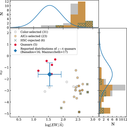
Figure 13. EW and αP
distributions of the candidates without J-band detection. The gray circles are the color-selected candidates, while the orange circles are the ones satisfying the AICc criterion (wq
> 0.99). Several candidates matched to the same quasar model were overlaid, so they appear to have low transparency on the diagram. The candidates covered by the HSC survey are marked by teal crosses. The five quasars in this work are shown as red circles. The blue diamond (and blue lines on the histograms) represents the reported normal distribution of z ∼ 6 quasars:  (Bañados et al. 2016) and αP
= −1.6 ± 1.0 (Mazzucchelli et al. 2017), in the form of mean ± standard deviation. Note that the correlation between the reported EW and αP
is not reflected in this figure.
(Bañados et al. 2016) and αP
= −1.6 ± 1.0 (Mazzucchelli et al. 2017), in the form of mean ± standard deviation. Note that the correlation between the reported EW and αP
is not reflected in this figure.
Download figure:
Standard image High-resolution imageRecent high-redshift quasar survey studies with deep HSC data have discovered some z ∼ 6 quasars with a strong but narrow Lyα line (EW > 200 Å; Matsuoka et al. 2018a,2018b, 2019a, 2022), but most of them are fainter than our survey limit (M1450 > −23.5 mag). Matsuoka et al. (2022) also showed that such faint quasars tend to have a strong Lyα line (or a high EW compared to continuum). Note that the EW values are estimated with the fixed continuum slope of αP
= −1.5 in those studies, so our EW values will increase if we assume the same condition. In addition, we cross-checked the reliability of the 31 candidates with deep HSC images. Only six of them are located in the HSC PDR3 survey area (teal crosses in Figure 13), but five of them have no matched sources even though they are bright enough to be detected in the HSC images. This means that such sources in our survey may be noncelestial bodies or artificial objects just detected in the  -band images. Even for the matched one (logEW = 1.9 and αP
= −4.5 ), it has a very blue color of
-band images. Even for the matched one (logEW = 1.9 and αP
= −4.5 ), it has a very blue color of  . Therefore, we conclude that these additional candidates without J-band detection are unlikely to be real high-redshift quasars.
Footnotes
- 12
- 13
- 14
The area size was updated from that of Kim et al. (2020; 85 deg2) with a slight increase.
- 15
- 16
The expected number density is calculated by integrating the LBG LF of Harikane et al. (2021) down to M1450 = −24 (−23.5) mag, corresponding to
(23.5) mag. If we assume 100% completeness, we obtain the expected number of 0.7 (4.8) by multiplying the cosmic volume of our survey area. Like quasars, however, the survey completeness for LBGs is also expected to be very low at −24 mag < M1450 < −23.5 mag. Therefore, we ignore them in the selection process. - 17
- 18
- 19
- 20
- 21
F606W−F775W color in the Hubble Space Telescope/Advanced Camera for Surveys (HST/ACS) filter system.
