Abstract
RW Aur is a binary system composed of two young, low-mass stars. The primary, RW Aur A, has undergone visual dimming events (ΔV = 2–3 mag) in 2011, 2014–16, and 2017–2018. Visual and IR observations indicate a gray absorber that moved into the line of sight. This dimming is also associated with changes in the outflow. In 2017, when the optical brightness was almost 2 mag below the long-term average, we triggered a Chandra observation to measure the absorbing column density NH and to constrain dust properties and the gas-to-dust ratio of the absorber. In 2017, the X-ray spectrum is more absorbed than it was in the optically bright state ( ) and shows significantly more hot plasma than in X-ray observations taken before. Furthermore, a new emission feature at 6.63 ± 0.02 keV (statistic) ±0.02 keV (systematic) appeared, indicating an Fe abundance an order of magnitude above solar, in contrast with previous sub-solar Fe abundance measurements. Comparing X-ray absorbing column density NH and optical extinction AV, we find that either the gas-to-dust ratio in the absorber is orders of magnitude higher than in the ISM, or the absorber has undergone significant dust evolution. Given the high column density coupled with changes in the X-ray spectral shape, this absorber is probably located in the inner disk. We speculate that a breakup of planetesimals or a terrestrial planet could supply large grains, causing gray absorption; some of these grains would be accreted and enrich the stellar corona with iron, which could explain the inferred high abundance.
1. Introduction
The formation of stars and planetary systems from large-scale molecular clouds is a complicated process with many interacting components. After the initial collapse of the cloud, an accretion disk forms around the central protostar. Low-mass stars (<3 M⊙) at this stage are called classical T Tauri stars (CTTS), and their circumstellar disks are the sites of planet formation. Disks regulate the angular momentum of the star and may launch a disk wind. Typical disks contain a mass of 10−3 to 10−1 M⊙ and disperse within a few Myr (see review by Alexander et al. 2014), which also sets the timescale for planet formation. During their evolution, disks undergo large structural changes. In particular, grains grow to larger sizes and settle in the disk mid-plane, leaving a gas-rich disk atmosphere behind (see review by Andrews 2015).
Gas comprises the majority of the mass in a protoplanetary disk; it thus controls essential transport processes within the disk, such as angular momentum redistribution and dust grain motion. For example, gas affects grain growth through the coupling of gas and dust dynamics (Weidenschilling 1977; Takeuchi & Artymowicz 2001) as well as the thermal and chemical balance of the disk (e.g., Woitke et al. 2009). Images of T Tauri star disks often have asymmetries or gaps (Casassus et al. 2013; van der Marel et al. 2013; ALMA Partnership et al. 2015; Pohl et al. 2015; Andrews et al. 2016), so the distribution of grain sizes in the stellar environment differs significantly for different sight lines.
Stellar UV and X-ray emission ionize the upper layers of the disk, particularly the inner disk edge. These ions couple effectively to the star-disk magnetic field. On the disk surface, ions can be accelerated magneto-centrifugally into a disk wind, possibly dredging along dust particles from the disk. Outflows can be clumpy, presumably changing in response to the magnetic field or the stellar irradiation (Bans & Königl 2012; Ellerbroek et al. 2014). The winds remove angular momentum and allow accretion to proceed. From the inner disk edge, gas is funneled onto the star.
Recent space-based monitoring campaigns with COROT, K2, and Spitzer revealed many different types of variability in the lightcurves of CTTS on timescales as short as hours. Stars with periodic or quasiperiodic dips in their lightcurve (Günther et al. 2014a; Stauffer et al. 2015) are of particular interest. A well-known star of this type is AA Tau (Bouvier et al. 1999). The inner disk of AA Tau is seen very close to edge-on, the best explanation for which is that an asymmetric feature, such as a warp caused by a planet embedded in the disk, periodically moves through our line of sight. In addition, AA Tau has shown a multi-year dimming event wherein the visual extinction increased by 4 mag (Bouvier et al. 2013) along with an increased X-ray absorbing column density (Schneider et al. 2015a). The duration of the event and the variable line emission originating from the upper layers of the disk indicate a position in the disk at a radius of few au. This absorber has an ISM-like  ratio.
In this paper, we report on new observations of RW Aur, which is a binary system composed of two K-type stars with masses of 1.4 and 0.9 M☉ and an age close to 10 Myr (Ghez et al. 1997; Woitas et al. 2001). The binary components are separated by 14 (semimajor axis 200 au, period 1000 years; Csépány et al. 2017) and located at a distance of 140 pc (van Leeuwen 2007). We concentrate on the primary star, which is one of only a few sources with an X-ray detected jet (Skinner & Güdel 2014), indicating outflows in excess of 400 km s−1. The disk mass around RW Aur A is ∼0.001 M☉ (Andrews & Williams 2005). The disk has an intermediate inclination, with estimates varying from 45–60° (Cabrit et al. 2006; Rodriguez et al. 2018) up to 77° (McJunkin et al. 2013), possibly because the inner disk is warped (Bozhinova et al. 2016).
In a well-sampled lightcurve reaching back to about 1900, RW Aur AB has shown long-term variability and a short dimming event, e.g., a one-month dimming first observed in 1937 December and repeated every few decades (Berdnikov et al. 2017; Rodriguez et al. 2018), but it has shown multiple optical dimming events since 2011. The 2011 event lasted about half a year (Rodriguez et al. 2013), with a dimming of ΔmV = 2 mag. Another dimming event started in mid-2014, displaying ΔmV = 3 mag as opposed to its typical bright state (which had been stable for decades) around mV = 11 mag (Rodriguez et al. 2013). The stellar flux reached the bright state again in 2016 November and December before plunging into a new dimming phase. Lamzin et al. (2017) see indications that the egress from a dim state happens earlier in the IR than in the optical. Takami et al. (2016) find that veiling, a measure of how strongly the continuum from the accretion shock contributes to the optical flux, is stronger in the 2015/16 dimming of RW Aur than in the bright state; X-shooter data (Facchini et al. 2016) confirm this finding. On the other hand, Petrov et al. (2015) infer no changes in the accretion close to the star, but see increased wind signatures. At the same time, photometry indicates that the 2015 extinction in RW Aur A is gray up to at least the K band (Antipin et al. 2015; Schneider et al. 2015b), while a selective (reddening) AV = 0.44 mag is seen in the bright state (Antipin et al. 2015).
Cabrit et al. (2006) observed a stream of gas on the outer edge of the disk of RW Aur A, and Rodriguez et al. (2013) suggested the dimming event in 2011 to be caused by this stream passing the line of sight to RW Aur A. In ALMA observations, Rodriguez et al. (2018) confirm the detection by Cabrit et al. (2006) and identify multiple further streams. Modeling by Dai et al. (2015) showed that tidal interaction in the passage of its binary companion, RW Aur B, can cause such a stream to form. However, in the new 2016 dimming event, multiple signatures show variability arising from material close to the star instead. Shenavrin et al. (2015) report that both increased hot dust emission and optical spectroscopic signatures indicated that there was an increase in absorption by an outflow during the dim state in 2015 (Petrov et al. 2015; Bozhinova et al. 2016; Facchini et al. 2016). Coupled with the fact that mass accretion is more stable during this dim state (Takami et al. 2016), it appears that the recent dimming events can only be explained by phenomena close to the star.
RW Aur AB has been observed in X-rays several times. Güdel et al. (2010) present unresolved XMM-Newton data, but Chandra is required to resolve the two stellar components. The first Chandra observation was taken in 2013 (Skinner & Güdel 2014) when RW Aur A was in an optically bright state. Schneider et al. (2015b) obtained a second data set in 2015, catching RW Aur in an optically fainter state. Here, we report on a third data set observed in 2017, again in an optically dim state. RW Aur B is also a variable X-ray source, most likely due to coronal flares.
We describe our observations and data reduction in Section 2. We derive results in Section 3 and discuss them in Section 4. In Section 5, we go through several physical scenarios that might cause the observed signatures. We end with a short summary in Section 6.
2. Observations and Data Reduction
We present new and archival X-ray data from Chandra, archival data from XMM-Newton, and optical data from Chandra's aspect camera (ACA) and AAVSO long-term monitoring lightcurves extended into 2017. Details of the X-ray observations are listed in Table 1.
Table 1. X-Ray Observations
| Observatory | ObsID | Date | MJD | Exp. Timea | Live Timeb | Mode | RW Aur A | Contam. |
|---|---|---|---|---|---|---|---|---|
| (ks) | (ks) | Counts | Counts | |||||
| XMM-Newton | 0401870301 | 2007 Feb 21 | 54123.5 | 36.4 | 34.5 | Full Frame | Unresolved | |
| Chandra/ACIS-S | 14539 | 2013 Jan 12 | 56304.1 | 60.9 | 54.5 | 1/8 subarray | 801 | 22.3 |
| Chandra/ACIS-S | 17644 | 2015 Apr 16 | 57128.3 | 40.2 | 35.1 | 1/8 subarray | 44 | 20.1 |
| Chandra/ACIS-S | 17764 | 2017 Jan 09 | 57762.3 | 41.1 | 38.5 | Full frame | 173 | 18.2 |
| Chandra/ACIS-S | 19980 | 2017 Jan 11 | 57764.1 | 14.5 | 10.2 | Full frame | 36 | 4.5 |
Notes.
aTime from exposure start to exposure end. bLive time in Chandra, i.e., corrected for the dead time during readout. In XMM-Newton, we give the ONTIME, the sum of all good time intervals of the PN chip that detected RW Aur.Download table as: ASCIITypeset image
2.1. XMM-Newton X-ray Data
RW Aur AB was centered in the field of view from the XMM-Newton observation, but the count rate in the RGS is too low to analyze the grating spectrum. We reduced the data with SAS version 15.0.0, following the standard procedures to screen periods of high background flux. We extracted a source region centered on the unresolved binary (AB) with a radius of 30″ in the PN and MOS detectors. We selected source-free background regions on the same chip (avoiding the chip edges where noise can be higher) with a radius of 50″ in the PN and 105″ for the MOS detectors.
2.2. Chandra X-Ray Data
Observations were taken roughly two years apart, where the last observation is split into two orbits separated by two days. All processing is done with CIAO version 4.9 and CALDB 4.7.1. RW Aur B, the brighter member of the binary in X-rays, was bright enough to be at risk of pile-up in the 2017 observations. At the fluxes observed, however, the pile-up fraction is less than 5% even in the brightest pixel; previous data were taken in a 1/8 sub-array mode that reduces the field of view and the frame time to alleviate this problem. For RW Aur A, the focus of this paper, pile-up is not significant in any of the observations.
We limit our analysis to the energy band 0.3–9.0 keV. Apertures with radius 0.54 arcsec (covering 75% of the point-spread function—PSF) were used to extract spectra from RW Aur A and B. We measure the background flux from a large, source-free region on the same detector and find that the expected background flux in each source region is <0.2 counts in any one observation. The B component of the RW Aur system is much brighter in X-rays than the A component. Therefore, the wings of the PSF from RW Aur B contribute to the data extracted for RW Aur A, while the reverse contamination is not relevant. Thus, we define an annulus centered on RW Aur B with inner and outer radii of 1 and 2 arcsec, respectively, as in Schneider et al. (2015b). This corresponds to the radii covered by the extraction region of RW Aur A. We remove a segment of ±60° around the position of RW Aur A from this annulus and use the remaining area (Figure 1) to estimate the number of counts due to contamination by RW Aur B (column “Contam.” in Table 1). This is a small fraction of the counts from RW Aur A, except for ObsID 17644 (2015).
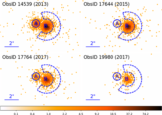
Figure 1. Images of RW Aur A and B in all four Chandra observations. We have marked the source region for RW Aur A (solid line) and the annulus (dashed line) designed to capture the contamination of the brighter RW Aur B by the wings of the PSF. The color scale shows counts per spatial bin. (The spatial bin size, 0.123 arcsec, in this image is smaller than the physical size of the ACIS pixels.) Note that the exposure time differs between observations, so the same number of counts does not represent the same flux.
Download figure:
Standard image High-resolution image2.3. Chandra Optical Data
Chandra has a small optical telescope in the aspect control assembly (ACA). This is a CCD detector with a wide bandpass from about 0.4 to 1.1 μm. The color conversion to standard filters is not calibrated for stars of arbitrary spectral shape. Only a few regions on the CCD are read out and transmitted to the ground. One of these slots was placed on the science target for ObsIDs 17644, 17767, and 19980. The image is intentionally defocused and RW Aur is not resolved. Aperture photometry is performed using the CCD noise model; see Nichols et al. (2010) for details.
2.4. AAVSO Data
We retrieved data for RW Aur from the database of the American Association of Variable Star Observers (AAVSO) in four bands: visual and standard V, along with the R and I filters. Many observers with different instrumental setups contributed to this data collection, but specifically the B, V, and R data close to the Chandra observations in 2017 are taken with a 684 mm aperture Keller F4.1 Newtonian New Multi-Purpose Telescope of the public observatory Astrolab Iris, Zillebeke, Belgium.8 The CCD detector assembly is a Santa Barbara Instrument Group STL 6303E operating at −20°C. The 9 μm physical pixels are read out binned to 3 × 3 pixels, which is 1.86 arcsec per pixel. The B, V, and R filters are from Astrodon Photometrics and have been shown to closely reproduce the Johnson/Cousins system. Differential photometry relative to stars in the field is conducted with the LesvePhotometry reduction package.
3. Results
3.1. Lightcurves
We first look at the long-term optical lightcurve and how the timing of the Chandra observations relates to the optical dimming events. Next, we turn to the Chandra count rates. Last, we present the lightcurve of the XMM-Newton observation, which includes a large X-ray flare but lacks dense optical monitoring.
3.1.1. Optical Lightcurves
Figure 2 (top rows) shows a long-term lightcurve of the RW Aur AB system. The first Chandra observation (marked by the first gray vertical line) took place during a bright state, which had been the long-term average for several decades, with mV ≈ 10.5 mag. The second Chandra data set was taken in an obscured state with mV = 12 mag in 2015. At the end of 2016, RW Aur AB briefly reached a bright state again, before fading back to mV = 11.7 during the Chandra observations in 2017 January. Later in 2017, the flux again climbed back to a bright state for a short time, just to drop again toward the end of 2017. Unfortunately, there is a gap of a few days in the optical data right around the Chandra observation. However, while RW Aur AB is known to have some variation on timescales of days and hours (Bozhinova et al. 2016), the lightcurve around the 2017 observations seems relatively smooth. The Chandra/ACA monitoring shows steady lightcurves with smooth variability on the 0.1 mag level during the observations, and a difference of about 0.2 mag between the two observations in 2017, which are about two days apart. Bozhinova et al. (2016) determine that the variability of RW Aur A on timescales of hours is irregular, which can be explained by changes in the accretion rate. Our data are consistent with this scenario, but the Chandra observations alone are too short to distinguish this from the periodic variability that hot (accretion) or cold (magnetic) spots would produce when they rotate in and out of view.
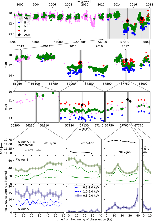
Figure 2. The top three rows show the optical lightcurve of RW Aur AB from AAVSO data. The system is not spatially resolved in these observations. Gray vertical bands mark the times of Chandra observations. “Vis.” are visual measurements without a standard filter, but the effective bandpass typically is fairly close to the V band. ACA is the band of the Chandra aspect control assembly. Bottom block: Chandra lightcurves from ACA (optical, unresolved), X-rays from RW Aur B (green), and X-rays from RW Aur A (blue). For clarity, error bars for 1σ uncertainties are only shown for the full band lightcurve. The increasing contamination on Chandra/ACIS means that a source with constant flux will produce a lower raw count rate in later observations. There are so few soft X-ray counts in RW Aur A in 2015 and 2017 that the dotted line falls almost exactly on the x-axis in 2015 and 2017. All lightcurves are background-subtracted and binned to one hour.
Download figure:
Standard image High-resolution imageWe interpolate the optical lightcurves to obtain values during the Chandra observation (Table 2). In 2015, there are observations within a few hours of the Chandra data in all bands. In all cases, the uncertainty is dominated by the variability of the target and we estimate the error on the optical magnitudes to 0.2 mag. Within this uncertainty, RW Aur AB is brighter by 0.5 mag in B, V, R, and the ACA band during the 2017 Chandra observation, compared with 2015. We do not see significant changes in the optical color between those observations.
Table 2. Optical Brightness (in mag) for RW Aur
| RW Aur | Ba | AB | ABb | Ac | Ac |
|---|---|---|---|---|---|
| year | 2014 | 2015 | 2017 | 2015 | 2017 |
| unit | mag | mag | mag | mag | mag |
| B | 14.5 ± 0.3 | 13.0 ± 0.2 | 12.5 ± 0.2 | 13.3 ± 0.3 | 12.7 ± 0.2 |
| V | 13.2 ± 0.3 | 12.2 ± 0.2 | 11.7 ± 0.2 | 12.8 ± 0.4 | 12.0 ± 0.3 |
| R | 12.3 ± 0.3 | 11.5 ± 0.2 | 11.2 ± 0.2 | 12.2 ± 0.5 | 11.7 ± 0.4 |
Notes.
aAntipin et al. (2015). bInterpolated between observations taken a few days before and after the Chandra observations. cThese values are inferred from the unresolved measurements of RW Aur AB by subtracting the RW Aur B flux from 2014, assuming that the flux from RW Aur B changes only on long timescales. See Section 3.1.1 for details.Download table as: ASCIITypeset image
None of the optical data presented here resolve the two components of the RW Aur AB system. Antipin et al. (2015) show that RW Aur B is also variable, but to a much lesser degree than RW Aur A. Comparing observations from 1994 and 2014, they find that RW Aur B has become brighter by about 0.7 mag, with almost no color variability. They suggest this to be due to a dust cloud with large grains moving through our line of sight, analogous to what is discussed for RW Aur A. We assume that this evolution is slow and subtract the long-term average of the RW Aur B fluxes (Table 2) to obtain the flux of RW Aur A. Within the uncertainties, we do not see changes in color. On the other hand, changes in B − V color are also possible, up to about 0.3 mag (1σ confidence range).
3.1.2. Chandra X-Ray Lightcurves
Figure 2 (bottom) shows X-ray lightcurves for both components of the RW Aur system and the ACA lightcurve where data exist. RW Aur B shows X-ray variability in every observation, but the average count rates are all similar. During the first observation, the flux increases smoothly by 30% and decreases by a similar amount in the second observation. In 2017, there is a short flare in the hard band that lasts about 5 ks. The second observation in 2017 shows rapid decline of the hard X-ray flux, possibly the tail end of a flare. Note that the count rate in the soft band is lower for the later observations because contamination builds up on Chandra/ACIS and the effective area declines between epochs. RW Aur A is fainter than RW Aur B in all observations. For RW Aur A, significant variability within an observation is seen only toward the end of the first observation in 2017 when the flux triples. The count rate in 2015 is more than an order of magnitude below the value seen in 2013 before the optical dimming started. In the 2017 observations, the count rate in the hard band again reaches the pre-dimming level, but essentially no signal is detected in the soft band.
3.1.3. XMM-Newton Lightcurves
The first half of the XMM-Newton observation in 2007 shows quiescent emission. A large flare erupted around 20 ks into the observation, with an increase in count rate by a factor of ∼20 (Figure 3). At the same time, the hardness ratio ( , where H is the count rate in the hard band of Figure 3 and S the count rate in the soft band) increases from −0.4 to 2.5 at the peak of the flare, before it decays back down to 0 at the end of the observation.
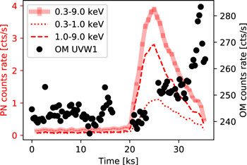
Figure 3. Count rates in the XMM-Newton observation in 2007, which did not resolve RW Aur AB. The X-ray count rate is mostly flat up to 20 ks, when a massive flare started. As in Figure 2, for clarity, error bars are shown only for the full-band lightcurve; they are comparable to the thickness of the line. In the flare, the count rate increases by factor of 20. The OM observed in a UV band (errors bars are smaller than symbols). There is an increase in OM count rate, but it rises several hours after the X-ray flare.
Download figure:
Standard image High-resolution imageWe compared the centroid of the X-ray emission in the quiescent and the flare phase, and they agree to about 01 (with statistical uncertainties of 0
4 and 0
2, respectively). The absolute astrometry of the XMM-Newton observation is insufficient to associate the centroid with either RW Aur A or B. If RW Aur A and B contribute to the quiescent emission, the pre-flare centroid would be located between them, close to the brighter component (in the Chandra observations, RW Aur B is always brighter than RW Aur A). RW Aur A and B are separated by 1
4. The count rate (and thus centroid of the detected events) is certainly dominated by the flaring source during the flare. So, if RW Aur A and B had equal X-ray brightness in the quiescent phase, the centroid position in the flare should shift by 0
7. A much smaller value is observed, and we thus conclude that the flare most likely occurs on the same component that dominated the quiescent X-ray emission. However, we cannot identify from the XMM-Newton observation whether this component is RW Aur A or B.
3.2. X-Ray Spectra
We first discuss the XMM-Newton data from 2007, where RW Aur AB is unresolved but we have the most signal (Section 3.2.1). Next, we turn to the Chandra observations, where RW Aur B (Section 3.2.2) and RW Aur A (Section 3.2.3) are spatially separated but the spectra from RW Aur A could be contaminated by the close-by, brighter RW Aur B. Of particular importance is a strong emission feature at 6.63 keV in the spectrum of RW Aur A in 2017, which we analyze in detail in Section 3.2.4.
We use the photospheric abundances given in Table 1 of Asplund et al. (2009) as reference throughout this paper. Uncertainties in this section are given as 90% confidence ranges.
3.2.1. 2007 XMM-Newton Data
The XMM-Newton spectra from RW Aur AB are displayed in Figure 4, separated into the quiescent phase (the first 20 ks of the observation) and the flare phase (after 20 ks); see Figure 3. Our spectral model consists of two optically thin, collisionally excited plasma model components (APEC, Foster et al. 2012) and a cold photoelectric absorber. We fit abundances in three groups of elements. We combine Mg, Si, and Fe into one group, because they all have very similar first ionization potential (FIP) values (7.6–8.1 eV). The FIP of Ne is 21.6 eV and is fitted on its own. We fix the abundances of elements with medium FIP values (S, O, N, and C all have FIP between 10 and 15 eV) to 1 because absolute abundances cannot be determined without grating spectroscopy; if we, for example, multiplied all abundances in the model by three and reduced the emission measure  (ni and ne are the ion and electron number density, respectively, which are integrated over the emitting volume V) by the same factor, the model would predict an almost identical spectrum. We investigated a possible change in NH or abundance between the quiescent and the flare phase, but did not see statistically significant differences. Therefore, we settled on a model where NH and abundances are the same in the quiescent and the flare phase. Furthermore, we coupled the temperature components, so that the fits in the quiescent and the flare phase have the same temperatures, but different emission measures. This simplifies the interpretation while still providing a good fit. The model thus has nine parameters: NH, the abundances of Ne and Fe, the temperatures of the cool and hot emission components, and the EM of the cool and hot components in the quiescent and flare phases. We fit the signal from the PN, MOS1, and MOS2 cameras on XMM-Newton simultaneously, using a χ2 statistic. The data are binned to 20 counts per bin. Fit results are shown in Table 3. The reduced χ2 of the model is only 0.7. Simpler models with fewer parameters (e.g., only one emission component with a single temperature) can still fit the data with a reduced χ2 around 1, but they show systematic deviations (e.g., the data below 1 keV is consistently underpredicted). Ergo, we chose to present the two-temperature model.
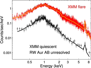
Figure 4. XMM-Newton/PN data with best-fit models in the quiescent and the flare phase. The RW Aur AB binary is unresolved. Data are binned to 20 counts per bin. Error bars in the plot are 1σ statistical uncertainties. The lines show the best-fit model with the parameters from Table 3.
Download figure:
Standard image High-resolution imageTable 3. Parameters of X-Ray Model Fits
| RW Aur | AB | AB | B | B | B | A | A | A | |
| Year | 2007 | 2007 | 2013 | 2015 | 2017 | 2013 | 2015 | 2017a | |
| Instrument | XMM | XMM | Chandra | Chandra | Chandra | Chandra | Chandra | Chandra | |
| Quiescent | Flare | Two-temp | One-temp | ||||||
| NH [1021 cm−2] | 2.62 ± 0.02 | 3 ± 1 | 1.1 ± 0.1 |
 c
c
|
400 ± 100c | 300 ± 100c | |||
| kT1 [keV] | 0.78 ± 0.04 | 0.38 ± 0.05 |

|
=0.6 |

|

|
|||
| EM1 [1052 cm−3] | 11 ± 2 | 45 ± 9 |

|

|

|
1.1 ± 0.4 |

|

|

|
| kT2 [keV] | 6.0 ± 0.3 | 2.0 ± 0.2 | =20 | =20 | =20 | ⋯ | |||
| EM2 [1052 cm−3] | 4.7 ± 0.5 | 128 ± 2 | 7 ± 1 | 9 ± 1 | 8 ± 1 | 1.0 ± 0.2 |

|
1.9 ± 1.9 | ⋯ |
| abundb: Fe | 0.12 ± 0.03 |

|

|
=0.5 |

|

|
|||
| abundb: Ne |

|

|
=1 | =1 | =1 | =1 | |||
red.  (DoF) (DoF) |
0.7 (1726) | 0.7 (251) | Cash statistic | ||||||
| observed fluxd | 4.7 | 78 | 3.0 | 4.5 | 3.3 | 1.2 | 0.2 | 2.7 | 2.9 |
intrinsic  e
e
|
30.3 | 31.4 | 30.1 | 30.3 | 30.1 | 29.5 | 29.0 | 31.6 | 30.6 |
Notes. Uncertainties are 90% Confidence Ranges.
aTwo different models are fit to the same data set; the first (two-temp) with two emission components at different temperature, the second (one-temp) with a single temperature. bRelative to solar abundances from Asplund et al. (2009). cThese numbers should be treated as lower limits. See Section 3.2.3 for discussion. dIn units of 10−13 erg s−1 cm−2 for the energy range 0.3–9.0 keV. Value is given for best-fit model without uncertainties. eIn units of erg s−1 for the energy range 0.3–9.0 keV. Value is given for best-fit model without uncertainties.Download table as: ASCIITypeset image
The 2007 XMM-Newton spectrum of RW Aur AB displays IFIP (inverse first ionization potential) abundances, where the abundance of elements with a high FIP (such as Ne) are enhanced and Fe is reduced, compared to solar abundances as seen in the Ne/Fe ratio. In the flare, the EM in the cool component increases by a factor of four while the EM of the hot component increases by almost a factor of 30.
The observed spectrum shows an emission feature around 6.7 keV (Figure 4) both before and during the flare. This feature is fully compatible with Fe xxv emission and is well-described by the plasma model fits. The hotter component of the plasma in the model is close to the peak formation temperature kT = 5.5 keV (k is the Boltzmann constant) of the Fe xxv 6.7 keV line. Given the higher EM in the flare, this feature is stronger there. Observing a 6.7 keV emission line from hot plasma is not surprising; we note this here only because the Chandra spectra show a feature at a slightly lower energy in 2017 that is discussed in detail in Section 3.2.4.
3.2.2. Chandra Spectra from RW Aur B
The three Chandra data sets from RW Aur B are qualitatively similar to each other (Figure 5); differences in the Chandra effective area at low energies are taken into account by using the appropriate ARF file in the fitting. Background is negligible in all cases. The two data sets from 2017 are treated separately in the fit, but we impose the condition that the fit parameters are identical for those two data sets (the data sets are merged only for display purposes in Figure 5). We fit the same model of one absorption component and two APEC plasma models that we used for the XMM-Newton data. Again, the value of the reduced χ2 is low, but if we reduce the number of model parameters (e.g., fit only one APEC component or fix the Ne and Fe abundance at solar values), we see systematic residuals in the fit.
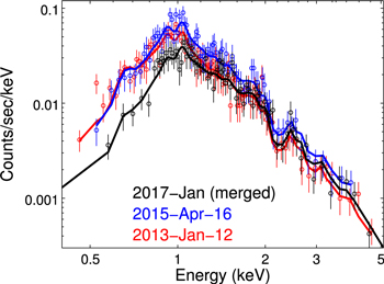
Figure 5. RW Aur B spectra extracted from Chandra data. Error bars in the plot are 1σ statistical uncertainties. The lines show the best-fit model with the parameters from Table 3. The spectra are very similar, except for the lower number of counts at low energies in the 2017 observation. This is due to increased contamination on the ACIS detector, and is taken into account in fitting.
Download figure:
Standard image High-resolution imageCompared to the XMM-Newton data with its prominent flare, the plasma temperatures are much lower. There is no plasma as hot as the component that gives rise to the 6.7 keV line in the XMM-Newton data. The absorbing column density and the abundance ratios are similar to the values found from the XMM-Newton data. It is therefore plausible that the XMM-Newton observation was dominated by emission from RW Aur B.
3.2.3. Chandra Spectra from RW Aur A
Chandra spectra from RW Aur A for the epochs 2013, 2015, and 2017 are shown in Figure 6. In 2017, RW Aur A is significantly brighter at high energies and shows a strong emission feature located at 6.63 keV (inset in Figure 7 and discussed in detail in Section 3.2.4) that is not seen in previous observations. At the same time, there is very little signal at soft energies after accounting for the contamination by the wings of the PSF from RW Aur B. We again fit a model with two thermal emission components and one absorption component. We add a model for the contamination by the RW Aur B PSF with the parameters of RW Aur B in Table 3 to each RW Aur A spectral fit. The normalization of these components is set to account for the small fraction of the RW Aur B PSF that falls into the RW Aur A spectral extraction region. We calculate a normalization factor from the counts observed in the dashed regions in Figure 1, then multiply it by the ratio of the areas of the RW Aur A extraction region and the dashed region. Because the total number of counts in the RW Aur A spectra is significantly lower than in the XMM-Newton data or in the RW Aur B spectra, we perform the fit using the Cash statistic (statistic cash in Sherpa; see Doe et al. 2007 and Cash 1979), which correctly accounts for the Poissonian likelihood in low-count bins—on the downside, it does not provide a goodness-of-fits statistic, such as the reduced χ2. As in Section 3.2.2, the data sets from 2017 are kept separate in the fitting process and are combined for display purposes only.
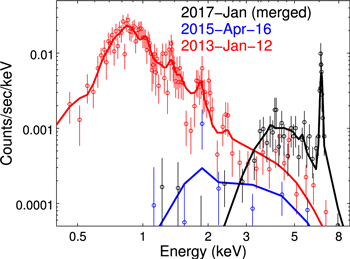
Figure 6. X-ray spectra for RW Aur A. Points are observational data and lines show models from Table 3 (for 2017, the “two-temp” model is shown). The two observations in 2017 are combined for display purposes only. All data are shown are background-subtracted, also for display purposes. Error bars indicate 1σ uncertainties.
Download figure:
Standard image High-resolution image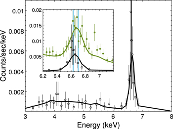
Figure 7. X-ray spectrum for RW Aur A observed in 2017 (combined from both observations for the purpose of presentation) with 1σ uncertainties and the best-fit model overlaid (Table 3, column “2 temp”). The inset zooms in on the emission feature centered on 6.63 keV. The olive-colored line in the inset represents data from the flare seen in XMM-Newton, scaled to the lower effective area of Chandra. Due to the emission in a hot flare, the continuum level is much higher and the emission feature is peaked at higher energies than the Chandra data. Vertical blue lines in the inset mark the energies 6.63 keV (the centroid of the feature in 2017) and 6.7 keV (the position of Fe xxv emission).
Download figure:
Standard image High-resolution imageThe decrease in soft (≲2 keV) X-ray flux from RW Aur A is the result of a variable absorbing column density whose extinction is higher in 2015 and 2017 than in the previously observed optically bright state (2013; red in Figure 6); the contamination of ACIS has a much smaller effect (compare to Figure 5).
Like Skinner & Güdel (2014), we find that a hot plasma component is required to fit the RW Aur A spectrum in 2013, but the temperature of this component is poorly constrained. Skinner & Güdel (2014) discuss this in detail and show that a power-law component actually gives a slightly better fit than a collisionally excited plasma, but we do not know of a physical process that could produce power-law emission in RW Aur A. Following Skinner & Güdel (2014), we fix the temperature of the hotter component at 20 keV. Furthermore, we find that the data insufficiently constrain the Ne abundance, so we fix this value at 1. Given the low signal in 2015, even more assumptions are needed to fit a model. We fix both temperatures and the Fe abundance at the numbers found for the 2013 data and leave only the absorbing column density NH and the normalization of the two emitting components for the fit. The fitted value for NH depends on these assumptions. For example, a cooler kT1 would predict more emission at lower energies and thus require a larger NH to explain the absence of signal below 1 keV. However, the fact that the observed flux dropped by two orders of magnitude or more below 1 keV (compared to the data from 2013), while the drop is less severe at higher energies, suggests a strongly increased NH. For a detailed discussion of the 2015 spectrum, see Schneider et al. (2015b).
In 2017, the spectrum is very different again (Figure 6). There is very little signal below 2 keV, while the flux >3 keV is several times stronger than in 2013 or 2015. In particular, there is a very strong emission feature between 6 and 7 keV, which is not seen in the previous Chandra data. This feature is discussed in detail in the next section. In Table 3, we show two different models for the 2017 data. First, we fit a model similar to those for 2013 and 2015 with a hot plasma component at 20 keV; this hot component has an EM comparable to the other data sets; however, the temperature of the cooler component is about twice the value seen in 2013, and the cool emission measure is about 50 times higher. Notably, an Fe abundance 15 times higher than in the Sun is required to match the emission feature between 6 and 7 keV. Such a large emission measure will also produce copious flux below 2 keV, and a very high absorbing column density of 400 × 1021 cm−2 is required to explain why we do not observe any flux in that region. Alternatively, we fit a model with just a single emission component at kT ≈ 3 keV. Due to the higher temperature, the Fe emissivity is higher and a smaller EM is sufficient to match the emission feature between 6 and 7 keV. Consequently, the best fit converges on a slightly smaller value for NH and an Fe abundance that is only five times solar—still an order of magnitude more than in 2013.
The photoelectric cross-section of all atoms and ions (in gas and small grains) in the line of sight contributes to the X-ray absorption. This is expressed as equivalent hydrogen column density NH, which is the total hydrogen column density of a gas with a solar abundance pattern. In the energy range between 2 and 3 keV where the observed flux drops (Figure 6), O, Ne, and Fe are the metals that contribute most to the total photoelectric absorption cross-section (Balucinska-Church & McCammon 1992). If these elements are enhanced by, e.g., one order of magnitude compared to solar abundances, then the true hydrogen column density is one order of magnitude lower than the equivalent hydrogen column density NH obtained from the fit. The value for NH is highly correlated with the temperature and the emission measure. A hotter and less absorbed plasma requires significantly less emission measure to produce the observed flux than a cooler and more absorbed plasma.
Still, the value for NH that we fit in either model for the 2017 data should be treated as a lower limit, because an absorbing column density this high will hide all signatures of cooler plasma in the spectrum. For example, we could add an extra emission component at 0.6 keV, the temperature seen in 2013, and concurrently increase NH without noticeably changing the predicted spectrum. In a large survey of T Tauri stars in the Orion nebula cloud, Preibisch et al. (2005) find that stars with a plasma component of kT ≈ 3 keV typically also have a cooler component around 1 keV with a comparable EM. If that is also the case in RW Aur A, the true NH might be even larger than the value given in Table 3 for 2017.
3.2.4. A Detailed Look at the Emission Feature in the RW Aur A 2017 Spectrum
A key feature observed from RW Aur A in 2017 is the emission feature between 6 and 7 keV. Figure 7 shows that spectrum on a linear scale to help locate this feature more precisely. We fit a Gaussian plus a constant to the spectral region 6.0–7.5 keV, using the Cash statistic on ungrouped data, and find that this feature peaks at 6.63 ± 0.02 keV (90% confidence interval of statistical uncertainty) ±0.02 keV (99% confidence interval of the absolute ACIS calibration9
). Statistically compatible results are obtained for fits with moderate binning (e.g., five counts per bin). This region is dominated by a complex of unresolved iron emission lines in the ionization stages Fe xxii to Fe xxv. The He-like triplet of Fe xxv at 6.7 keV dominates the emission if enough hot plasma is present (peak formation temperature for the lines is kT = 5.5 keV). The lower ionization stages have weaker lines, many of which are located at slightly lower energies. The peak of the emission feature seen in RW Aur A is at 6.63 keV, indicating that the temperature is too low to ionize iron up to Fe xxv. Fe xxv has several lines in the 6.6–6.7 keV range, but the 6.70 keV line is always the strongest one. Thus, if Fe xxv were present, the centroid would be close to 6.70 keV. For comparison, an equivalent fit to the XMM-Newton data from 2007, where a similar feature is observed, finds the peak at  keV (90% confidence interval of statistical uncertainty) ±0.01 keV (absolute PN and MOS calibration Smith 2016)), which is compatible with Fe xxv emission.
The model for this feature (Figure 7) is asymmetric because several unresolved Fe lines from different ionization stages contribute to the emission. The emissivity of this iron feature drops by several orders of magnitude over a small range of temperatures. So, for temperatures at the lower end of the confidence interval, higher iron abundances would be required to match the observed flux at 6.63 keV. That is why the “two-temp” model in Table 3 requires a higher Fe abundance than the “one-temp” model. In the “two-temp” model, kT1 is lower and thus the emissivity of Fe is lower than in the “one-temp” model. The position of the observed peak directly rules out a significant contribution from highly ionized iron, and thus an Fe abundance significantly above solar and at least an order of magnitude higher than in 2013 is needed, independent of the choice of parameterization (e.g., number of temperature components) for the global model.
In the Appendix, we split the data from 2017 into three phases, but do not find any significant time evolution. In particular, the Fe emission feature is observed at all times; it is not a feature caused by the small flare at the end of ObsID 17764 that can be seen in the lightcurve in Figure 2.
4. Discussion
The optical properties of RW Aur AB during the 2016/2017 dimming event are similar to the previous dimming observed from 2014 to 2016. The B − V and V − R colors are also similar, and the depth of the dimming is 0.5 mag less than before. In fact, from optical observations alone, it is not clear if the new dimming is an unrelated event or a continuation of the dimming that started in 2014 with a short gap in the absorbing material. Similarly, in X-rays, we find that NH increased by a factor of 70 in 2015 and a few hundred in 2017 or so (the exact number depends on the plasma model). On the other hand, in 2017, there is significantly more emission around 5 keV and the Fe abundance is about one order of magnitude higher than in either the optically bright state in 2013 or the optically faint state in 2015.
In this section, we derive limits on the gas and dust mass, distribution, as well as abundance based on these measurements. In Section 5, we will then discuss which physical processes could cause the changes in gas and dust properties.
4.1. Where is the Absorbing Column Density Located?
For the following discussion, it is important to remember that the true hydrogen column density could be lower than the fitted NH, if elements such as O, Ne, and Fe, which dominate the absorption between 2 and 3 keV, are enhanced compared to solar abundances.
Using the depth of several optical absorption lines, Facchini et al. (2016) placed a limit on the gas phase column density of Na i of  . Using solar photospheric abundances, we can convert this to
  . This is about one order of magnitude below the NH value we observed in 2013, and two to three orders of magnitude below the NH we fit in 2015 and 2017, indicating that almost all of the gas in the line of sight must be ionized. Na in a low ionization state would be missed in the Na i measurement, but result in same X-ray measured NH as neutral Na.
4.1.1. Are We Looking through the Disk?
Cabrit et al. (2006) observed the disk of RW Aur A in  and
and  lines with radio interferometry. This allowed them to place limits on the column density of warm gas in the disk of
  in the inner 100 au. Their upper limit is close to our measured NH and there might be an additional cold gas component in the disk mid-plane that is unseen in the radio observations. Thus, a sightline through the disk is compatible with our observed value for NH in 2017. The problem with this scenario is that the disk has an intermediate inclination, so the sightline to the central star does not pass through the plane of the disk unless the inner disk is massively warped. To make matters worse, any sightline though the disk should contain some small dust grains, in contrast to the observed gray absorption (see discussion on the
  ratio in Section 4.2).
4.1.2. Are We Looking through a Disk Wind?
The model fits to the 2015 and 2017 epochs indicate an extremely high absorbing column density of >1023 cm−2. During the 2014–2016 fading, Facchini et al. (2016) and Takami et al. (2016) detected increased blueshifted Ca ii absorption, indicative of an increasing mass outflow, and they also identify a much stronger [O i] 6300 Å emission line, which is formed in the outflow, compared with spectra taken in the optically bright state. Bozhinova et al. (2016) argue that this wind also carries the dust that causes the gray absorption, although it is not clear if a wind could drag up sufficiently large dust particles from the disk to appear gray (Owen et al. 2011). If this wind is strong within the dust evaporation radius, that could provide a large gas column density without any accompanying optical reddening.
As an order-of-magnitude estimate, we assume that we are looking through a uniform disk wind emanating from the inner 10 au of the disk and that the line of sight does not pass through the disk itself. In order to reach the measured NH value along the line of sight, the density in that region has to be 2 × 109 cm−3. Even for a modest outflow velocity of only 10 km s−1 this would result in a mass loss rate of more than  . If that is true, a new knot will become visible in RW Aur A’s jet very soon. On the other hand, such mass loss cannot be sustained for very long and would be significantly larger than the mass accretion rate of
  measured in the previous dimming. Facchini et al. (2016) even detected a reduced accretion rate in the photometrically dim state, but caution that part of the accretion region could be eclipsed.
4.1.3. Are We Looking through a Screen?
A more plausible scenario is that the absorbing column density is not outflowing and the new absorber in 2017 is at least large enough to cover the stellar disk. We can derive a gas mass of
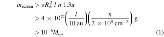
where u is the atomic mass unit and  is the average particle mass. Here, l is the thickness of the screen and n is its particle number density. If the disk is inclined, these masses are easy to explain but they also roughly match the mass of an 80 km size planetesimal, close to the initial planetesimal size (Morbidelli et al. 2009). For comparison, this is more than the mass of the Martian moon Phobos (1019 g, Pätzold et al. 2014), but still five orders of magnitude below the mass of Mercury, the smallest inner planet in our solar system (4 × 1026 g). Similar estimates have been made to explain the added absorption in TWA 30 and T Cha where Principe et al. (2016) and Schisano et al. (2009) calculate 5 × 10¹⁹ g and 4 × 10²⁰ g, respectively. These calculations only give an order-of-magnitude estimate for a lower limit to the total mass in this region, because the absorber might be much larger than just the size of the visible star. If the mass is provided by the break-up of a planet or planetesimal, the resulting dust cloud would shear out into a ring and mscreen would represent only a very small fraction of the total mass. Furthermore, the variability within a dimming event in the optical lightcurve in Figure 2 suggests that the absorber is not homogeneous.
4.2. The  Ratio
Ratio

Figure 8 shows how the  ratio for RW Aur A changes with time. The selective reddening for RW Aur A in the optically bright state corresponds to a visual extinction of AV = 0.44 (Antipin et al. 2015), and for 2015 and 2017 we add the additional gray extinction seen as ΔmV between the long-term average mV and the mV in Table 2. As outlined in Section 1, the additional absorber in the dim phases of RW Aur A seems to be gray in the optical photometry; in other words, it is not wavelength-selective, because it blocks the light completely. This can be caused by either a screen of large particles, such as large dust grains or planetesimals, or by a layer of gas and dust with such a high column density that it is optically thick at all relevant wavelengths. In the latter case, however, there has to be a fairly sharp edge between the optically thick absorber, which blocks part of RW Aur A, and the open space through which we see the remaining flux from RW Aur A. In the X-rays, we do not know the true intrinsic source flux. Thus, we cannot reference the previous observations to estimate the true flux, as we do in the optical. It is possible that the gray absorber reduces the overall flux of X-rays in addition to the gas column density NH changing the spectral shape.
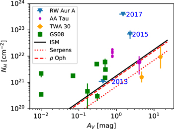
Figure 8.
 ratio for RW Aur A in the three epochs (see text in Section 4.2 for a description of how AV was estimated for RW Aur) in comparison to AA Tau (the small dots without error bars are measurements before the dimming) and TWA 30, as well as the sample from Günther & Schmitt (2008) (GS08 hereafter). The
  ratio observed in the ISM and the average value for two other star-forming regions are also shown. See text in Section 4.2 for data sources. Optical and X-ray data for RW Aur A, AA Tau, and TWA 30 are contemporaneous, while the remaining data (GS08, ISM, Serpens, and ρ Oph) are based on optical and X-ray data taken non-contemporaneously.
Download figure:
Standard image High-resolution imageFigure 8 also shows two other CTTS where NH and AV variability has been seen. AA Tau used to show variability of NH within its eight-day cycle, while the change in AV over the cycles was not significant (Grosso et al. 2007). The figure shows these data points as small dots without error bars. Data for AA Tau’s 2013 dimming event are taken from Schneider et al. (2015a). TWA 30 also has a time-variable  ratio (Principe et al. 2016), but is different from RW Aur A and AA Tau in that it presents a lower
  ratio than the ISM similar to the Serpens cloud. Moreover, for TWA 30, the values of NH and AV change with time, but the
  could be the same. The two epochs of contemporaneous optical/X-ray observations are separated by more than a month, so the additional absorber can be located well outside the dust sublimation radius. We see TWA 30 nearly edge-on, so the measurements probe the composition of the disk where we expect evolved grains, unlike RW Aur.
For the remaining samples in the figure, NH and AV are measured non-simultaneously. Vuong et al. (2003) compared NH and AV for six nearby star-forming regions, including the Orion Nebula Cloud (ONC). For the ρ Oph star-forming region, they find an  significantly below the ISM value. They interpret this as a sign that the cloud material has a lower metal abundance than the ISM, consistent with recent solar abundance measurements. Alternatively, grain growth can increase the amount of extinction per unit mass until the grains reach 1 μm in size (Ormel et al. 2011). Grain growths is also the scenario preferred by Winston et al. (2007) to explain the
  ratio seen in the Serpens cloud, where
  is less than half of the ISM value of
  (Predehl & Schmitt 1995).
Günther & Schmitt (2008) analyzed older, but still accreting CTTS in low-mass, star-forming regions. They found consistently high  ratios, indicating gas-rich material or massive grain growth. Some of these sources could be seen through the accretion column located very close to the central star, where small grains evaporate. This is also consistent with observations of AA Tau, where the eight-day periodicity proves that the absorber with high
  ratio is located close to the star—whereas the new absorber, which has a more ISM-like
  ratio, appeared on a much longer timescale, and thus must be located at a larger distance from the star, outside the dust-sublimation radius. RW Aur A has a fairly large accretion rate, so there must be enough mass in the inner disk region, and possibly even within the dust-sublimation radius, to provide a large gas column density. However, there are no indications that the accretion rate changes significantly between the dim state and the bright state (Facchini et al. 2016). Thus, the increased NH points to a change in the geometry rather than in the accretion rate.
4.3. The Extra Emission Measure
The Chandra X-ray and optical lightcurves of RW Aur A (Figure 2) in 2017 are mostly flat, and the fact that a similar flux level was observed two days later shows that the observations were not taken during a big flare. Thus, the increased emission at energies above 3 keV in 2017, compared to 2013 and 2015 (Figure 6), must be due to a different structure of the emission region.
The energy of emission from shock-heated material is limited by the velocity jump across the shock front. For the mass and radius of RW Aur A (White & Ghez 2001; Dodin et al. 2012), the freefall velocity is <500 km s−1, and thus the temperature of the shock is <0.3 keV. The relatively soft X-rays observed by Skinner & Güdel (2014) in the resolved jet show that shocks in the outflow reach similar temperatures. Because the temperature of the observed plasma in 2017 is considerably larger, it must be magnetically heated in the corona.
4.4. Fluorescent Iron?
When iron is ionized by high-energy photons, an inner electron from the K-shell can be removed. Fluorescence occurs when an electron from a higher level (usually L) recombines to fill the K-shell. The energy of the fluorescent emission depends on the charge state of the ion. For neutral iron or ions in a low ionization stage, the energy is around 6.4 keV. Only for highly ionized Fe does this line reach an energy similar to the feature we observe in the 2017 observation of RW Aur A (Fe xxiii: 6.63 keV, Kallman et al. 2004). Fluorescent Fe emission is sometimes seen in CTTS when very bright flares occur and provide a high X-ray flux that ionizes neutral iron in the accretion disk or funnels (e.g., Tsujimoto et al. 2005; Czesla & Schmitt 2007; Hamaguchi et al. 2010). In RW Aur A, we see a feature centered on 6.63 keV. If this is a fluorescence line, the source of it is so highly ionized that it must be located in the stellar corona; at the same time, the source of the ionizing radiation must be hidden from view, because we do not detect a 6.7 keV feature. Thermal emission from a range of Fe species (mostly Fe xxii–Fe xxiv), as discussed in Section 3.2.4, is a simpler and more likely explanation for the observed spectrum.
4.5. The Fe Abundance
The best model fit to the X-ray spectrum of RW Aur A in 2017 in Table 3 (model “two-temp”) shows an Fe abundance, compared to solar, of ∼15 and an emission measure of 50 × 1052 cm−3. An increase in iron abundance is not compatible with the properties of an active stellar corona. There is some element differentiation in coronae, where elements of low FIP such as Fe are enhanced in stars with low activity and depleted in stars with a high activity level (see review by Güdel 2004, and references therein). RW Aur A had a low Fe abundance in 2013, which is compatible with this picture. However, there is significantly more emission at high temperature in 2017, indicating a higher level of activity, and thus the Fe abundance should have decreased instead of increased. We use the EM and abundance to estimate the total mass of iron in the emitting material, which is inversely proportional to the assumed density. To simplify the estimate, we assume that the emitting volume V is filled by plasma with a constant ion number density n and an electron density  , where 1.4 is the average number of electrons released per ion. We can then write
  . We calculate the total mass of Fe by multiplying the total number of Fe ions times the average weight of an Fe ion (55.8 u), where u the atomic mass unit.

Assuming a typical coronal density of  (Ness et al. 2004), the reference Fe abundance from Asplund et al. (2009), and the values for EM and relative Fe abundance fitted in Table 3 (2017, column “two-temp”), only about 3 × 10⁻¹⁰ Earth masses of iron are required in the emitting plasma. Because the plasma temperature rules out an origin in the accretion shock, any accreted mass must be transferred to the corona in some way. Observations of RS CVn EI Eri suggest that the timescale of element fractionation in active regions is a few days (Nordon et al. 2013); similarly, the timescale on which mass lost to the solar wind is replaced is one to two days (Laming 2015). Assuming that one day is also a reasonable estimate for the time that accreted iron remains in the corona before it is mixed in the convective zone or ejected into the stellar wind, and assuming that the abundance we observe is typical for the most recent dimming starting in 2016, about 10−7 earth masses of iron have passed through the corona. A planetesimal could easily supply this reservoir. At an age of <10 Myr (White & Ghez 2001), the convection zone of RW Aur A is still so deep that it contains about half of the total stellar mass (Serenelli et al. 2011); the convective turnover time is on the order of one year (Landin et al. 2010). Thus, Fe would accumulate in the upper photosphere until it reaches a maximal concentration after about one year.
5. Scenarios
We are looking for a unified model that explains the variable absorption, Fe abundance, and increased volume of magnetically heated plasma. The most obvious explanation for additional flux at high energies in an active star is a large coronal flare (e.g., Favata et al. 2005). However, the X-ray and optical light curves during the observations in 2017 show no indication of a flare. Also, coronal flares induce little change in NH, in contrast to our observations. In the following sub-sections, we discuss other scenarios; a planetesimal breaking up or puffing up the inner disk seems to be most consistent with the data.
5.1. Can This Be Explained by the Tidal Stream?
Rodriguez et al. (2013) suggest that the dimming event in 2011 could be due to the tidal stream between RW Aur A and B passing through the line of sight. However, many of the features observed in the more recent dimming events can only be explained by variable phenomena near the location of the inner disk and/or the disk wind close to the star (e.g., Petrov et al. 2015; Shenavrin et al. 2015; Bozhinova et al. 2016; Facchini et al. 2016; Takami et al. 2016), which is consistent with the data presented here: a stream of gas and dust passing by at a large distance from the star cannot cause the changes in the emission region needed to explain the increased hot emission and the Fe abundance inferred from X-ray spectral modeling (Section 3.2.4). Strictly speaking, this does not rule out the possibility that the 2011 event was caused by the tidal stream passing through our line of sight and any later dimming being due to an unrelated mechanism, but given the long-term stability of the lightcurve before 2011 (Rodriguez et al. 2013), it seems more likely that all dimming events are related in some way.
5.2. Planetesimal Breakup in the Inner Disk
Circumstellar disks are the sites of planet formation. As part of this process, dust grains coagulate into larger aggregates, and eventually into planetesimals and planets. When two particles collide, they may either stick together or break apart. Typical disk lifetimes are a only few Myr (see review by Alexander et al. 2014), but RW Aur A still has a disk at an apparent age of 10 Myr (Woitas et al. 2001), so the system certainly had enough time to form planets; given the long timescale, it may even have formed more planets or planetesimals than typical.
A possible scenario is that two large planetesimals collided in 2011 and released a cloud of smaller particles, which caused the optical dimming. After about six months, the particles are no longer visible because they are accreted onto the star or settled into the disk midplane.
However, some larger fragments of the collision may remain, and the collision may have set them on eccentric orbits that increase the probability of further collisions after the initial event. We speculate that collisions caused the dimmings in 2014 and possibly again at the end of 2016. The products of each collision depend on the composition of the colliding planetesimals and the impact parameter (Windmark et al. 2012). Collision products can collide again and cause a cascade that breaks up particles, reducing them to micrometer sizes (Krijt & Kama 2014). If the size distribution is skewed to particles that are larger than μm-sized, this will cause gray absorption in the optical. At the same time, the newly released dust will increase the opacity of the disk in layers that were optically thin before. This leads to more energy absorption and rising temperatures, which will increase the scale height of the disk, pushing the limits of optically thick absorption to even greater heights. Detailed modeling is needed, but this is at least consistent with the observed increased optical and X-ray column density.
We can estimate the dust mass in the line of sight, assuming spherical dust grains with radius a and mass density  distributed over a length l with a number density n. They will reduce the flux by a factor
  . The optical light curve shows a dimming of ΔV = 2–3 mag, about a factor of 10. As a minimum, the dust column covers the stellar disk, so a lower limit to the dust mass Md of the gray absorber is

For grains with a = 0.1 mm, the dust mass is 1/100 of the gas mass estimated from the NH in Table 3 (column 2017, “two-temp”), assuming solar abundances in the absorbing material—i.e., a mean particle mass of 1.3 u. This ratio is similar to common ISM values. However, for a particle size distribution  , a in the equation above is replaced by
  , where a0 is the smallest particle (we take 0.1 mm) and a1 is the largest particle. Neither a0 nor a1 are well-known, but a1 = 1 km is a reasonable scale for the breakup of a planetesimal, which would lead to an Mdust that matches the gas mass from NH within a factor of a few.
The X-ray spectrum taken in 2015 did not show any peculiar Fe feature, and emission in general was fainter than in 2017. Either accretion of Fe is intermittent, or the collision that caused the 2017 dimming event happened to include a more iron-rich planetesimal than the previous events. RW Aur A is old enough that considerable planetary migration may have occurred (e.g., Tanaka et al. 2002). Thus, the inner disk region may contain planets or planetesimals that formed in different regions of the disk and therefore have different compositions.
5.3. Context for a Planetesimal Breakup Scenario
Detailed hydrodynamical models of the disk and planetesimal for the scenario discussed here are beyond the scope of this paper, but we can constrain the location of the event by comparing the timescale of the changes in the lightcurve to the timescale of the relevant physical processes in the disk. The optical dimming observed in 2011 lasted six months. Another dimming event started in 2015 and lasted until at least the end of 2017, showing only short spikes in the lightcurve up to the bright state level. X-ray observations have been done about every two years, and the plasma properties have changed significantly between them.
Assuming that the first breakup is due to a collision around 2011, it could have set fragments onto eccentric trajectories. For RW Aur A, the Roche limit is about 2 R*, which is well within the co-rotation radius. In the magnetically funneled accretion scenario, the stellar magnetic field couples to the disk around the co-rotation radius and little gas or particles exist inside for more than about one orbit. Thus, we expect that the planetesimal breaks apart due to collisions, not tidal interaction with the central star. Collisions in 2011 and 2015, which release clouds of gas and dust, might have caused the dimming and increase in NH from 2015 on. Could this also explain the sudden increase of the Fe abundance? In a circumstellar disk, the gas rotates at slightly sub-Keplerian velocities because it is supported by gas pressure. On the other hand, dust particles need to rotate at Keplerian velocities to maintain a stable orbit. Thus, they feel a headwind and migrate inward; the rate of this migration depends on their Stokes number. The radial drift time for particles is a few hundred orbits, so drifting from a radius just slightly outside the co-rotation radius to the inner edge of the disk (where gas and particularly iron-rich particles couple to the magnetic field and are accreted) could happen in about 1.5 years (Birnstiel et al. 2016) for particles with a Stokes number around 1 (Brauer et al. 2008). This corresponds to a radius of  m, where Σg is the gas surface density of the disk and we have used
 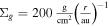 at disk radius r. The value of Σ close to the star is not well-known. The value of
  at 1 au is lower than those typically estimated for T Tauri disks (Andrews et al. 2010) and higher than those expected for the disk mass estimates in the RW Aur A simulations of Dai et al. (2015).
Under these assumptions, the first particles from the 2015 fragmentation just made it onto the central star in 2017. It is not unreasonable to infer that those fragments originated in the compact core of the original planetesimal and are iron-rich. We should see enhanced accretion in the coming years as both larger and smaller fragments pass through the disk and are accreted. Rodriguez et al. (2018) point out that earlier dimming events occurred in 1937 and 1987, so collisions of this type might be common in the RW Aur A disk due to the disturbance from RW Aur B.
A scenario that essentially requires the accretion of a planetesimal or (part of) a terrestrial planet is not without precedent. While this has never been observed directly in young stars, there are several white dwarfs whose surface abundances show clear signatures of ongoing accretion of debris from a terrestrial planet (Jura 2006; Farihi et al. 2009; Melis et al. 2011; Gänsicke et al. 2012).
5.4. Other Scenarios
The precession timescale for a disk similar to RW Aur should be about 0.5 Myr at 40 au (Owen & Lai 2017), which is 2800 orbits. Even when scaling this down to the co-rotation radius, that still predicts a scale of 80 years; furthermore, such precession should be periodic, but RW Aur A’s lightcurve before 2011 did not show disk eclipses for at least one century.
There is, however, a possible scenario that shares many characteristics with a planetesimal breakup: a pressure trap. Thick disks can contain deadzones where the ionization is so low that the magnetic field does not couple to the disk material. Pinilla et al. (2016) show that particles of >1 mm will be trapped on the outside of a deadzone. If the disk structure changes, e.g., responding to an inward-traveling wave excited by the tidal forces of RW Aur B passing by (Dai et al. 2015), and that trapped material is released, this might supply enough large grains to explain the extra absorber. As in the planetesimal collision scenario, particles of a certain size would move inward and supply the Fe seen in the X-ray emission. If this is true, the accretion rate in RW Aur A should increase significantly in the next few years as the bulk of the mass reaches the inner disk edge.
Last, we note that radial velocities of several 1000 km s−1 would be required to explain the 6.63 keV feature as a redshifted 6.7 keV Fe xxv line. This is an order of magnitude faster than the fastest known jet component in RW Aur. Skinner & Güdel (2014) observed X-ray emission from the jet, which requires just a few hundred km s−1 for shock-heating (e.g., Günther et al. 2014b).
6. Summary
We present new Chandra data regarding the binary RW Aur. The resolved binary member RW Aur A had several optical dimming events between 2011 and 2017. Previously published Chandra data show RW Aur A in an optically bright state and in a previous dimming event. We find that RW Aur A has an exceptionally high absorbing column density of a few  in 2017, orders of magnitude more than in the optically bright state. We also see significantly enhanced emission in the hard X-ray range above 3 keV, and a newly appeared Fe emission feature at 6.63 keV that indicates an Fe abundance one order of magnitude above solar. The temperature of the plasma is too high to be shock-heated; the most plausible location for it is an active corona. Significant accretion of iron-rich material is required to boost the abundance to the observed value. We speculate that the breakup of a terrestrial planet or a large planetesimal might supply the gray extinction seen in the optical and the large amount of gas column density observed as NH in X-rays; it may also provide iron in the accretion stream to enhance coronal abundances.
We thank an extremely thorough and detail-oriented referee for numerous suggestions that led to substantial improvements in the manuscript. The scientific results reported in this article are based on observations made by the Chandra X-ray Observatory. We gratefully acknowledge the variable star observations from the AAVSO International Database that were contributed by observers worldwide, and in particular the BAAVSS. This research has made use of software provided by the Chandra X-ray Center (CXC) in the application packages CIAO, ChIPS, and Sherpa. Support for this work was provided by the National Aeronautics and Space Administration through Chandra Award Numbers DD5-16077X and GO6-17021X issued by the Chandra X-ray Observatory Center, which is operated by the Smithsonian Astrophysical Observatory for and on behalf of the National Aeronautics Space Administration under contract NAS8-03060. T.B. acknowledges funding from the European Research Council (ERC) under the European Union’s Horizon 2020 Research and Innovation Programme under grant agreement No 714769. P.C.S. acknowledges support by DLR grant 50 OR 1706.
Facilities: CXO(ACIS - , ACA) - , AAVSO - .
Software: astropy (Astropy Collaboration et al. 2013), CIAO (Fruscione et al. 2006), Sherpa (Doe et al. 2007).
Appendix: Time-resolved Analysis of the RW Aur A Chandra Data from 2017
Figure 2 shows that the count rate in RW Aur A increases toward the end of the first observation taken in 2017; this might be due to a coronal flare. An intuitive approach is to search for time variability in the X-ray spectrum, particularly with an eye toward discerning whether the Fe emission feature is correlated with that flare. This appendix complements the analysis in Sections 3.2.3 and 3.2.4.
We split the longer of the two observations (ObsID 177654) in 2017 into two parts, a “pre-flare” block (up to 30 ks) and a “flare” block (after 30 ks). We then fit those two spectra and the spectrum from ObsID 19980, which was taken two days later, with a model similar to the one used in Section 3.2.3. Because the count rate in each of the three spectra is low, we use the Cash statistic on ungrouped data and only present fits for a model with a single temperature component. We use the same background model as in Section 3.2.3, i.e., we describe the contamination from RW Aur B with the model fit for 2017 in Table 3 and a single scale factor to account for the fact that only a small fraction of the RW Aur B PSF falls into the extraction region of the RW Aur A spectrum. RW Aur B is moderately variable in 2017, but the variability appears not to be correlated with RW Aur A. Furthermore, the signal from RW Aur A is so low that the uncertainties of the fitted parameters are much larger than any change that would be introduced by relatively small changes in the background model.
Figure 9 shows the observed data and the best-fit models. Model parameters are listed in Table 4. The signal is weak in all three spectra. The figure shows marginally stronger emission in the 3–5 keV range in the “flare” spectrum than in the other two spectra, which is consistent with the interpretation that the increase in flux in the lightcurve towards the end of ObsID 17764 is related to stellar activity. Figure 9 indicates that the Fe emission feature at 6.63 keV is present in all spectra, but the low signal makes this hard to see in the binned data shown in the figure.
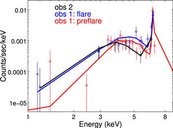
Figure 9. X-ray spectra for RW Aur A in 2017. Points are observational data and lines show models from Table 4. The first observation in 2017 (ObsID 17764) is split into a “preflare” state (the first 30 ks of the exposure) and a “flare” state (the remaining exposure). The second observation is ObsID 19980. Observations are binned to five counts per bin and background-subtracted for display purposes. Error bars indicate 1σ uncertainties.
Download figure:
Standard image High-resolution imageTable 4. Parameters of X-ray Model Fits for RW Aur A in 2017. Uncertainties are 90% Confidence Ranges
| ObsID | Combined | 17764 | 17764 | 19980 |
|---|---|---|---|---|
| “One-temp” from Table 3 | quiescent | flare | obs 2 | |
 [1021 cm−2] [1021 cm−2] |
300 ± 100 |

|

|

|
| kT1 [keV] |

|

|

|

|
| EM1 [1052 cm−3] |

|

|

|

|
| abundb: Fe |

|

|

|

|
| abundb: Ne | =1 | =1 | =1 | =1 |
| statistic | Cash | |||
| observed fluxc | 2.9 | 2.6 | 8.7 | 1.6 |
intrinsic  d
d
|
30.6 | 30.8 | 30.5 | 30.9 |
Notes.
aThese numbers should be treated as lower limits. See Section 3.2.3 for discussion. bRelative to solar abundances from Asplund et al. (2009). cIn units of 10−13 erg s−1 cm−2 for the energy range 0.3–9.0 keV. Value is given for best-fit model without uncertainties. dIn units of erg s−1 for the energy range 0.3–9.0 keV. Value is given for best-fit model without uncertainties.Download table as: ASCIITypeset image
The best-fit values vary between the three spectra, but uncertainties are so large that all three fits are still compatible with each other. The numbers highlight some of the ambiguities in the fits. For example, while the best-fit kT increases in the flare, the derived intrinsic LX in the flare is actually lower than the pre-flare LX because the fitted pre-flare NH is also larger. Similarly, we can see the strong dependence of the Fe abundance on the fitted temperature. The fit for the “flare” phase has such a large best-fit temperature that Fe is ionized so highly that little Fe xxv remains; thus, a very large Fe abundance is needed to explain the emission feature. On the other hand, the fit for ObsID 19980 is cool enough to have Fe in the appropriate ionization stages, and consequently the fit gives a lower Fe abundance. Again, the values are compatible within the uncertainties. Some of this is due to our simple model with a single temperature emission component, whereas we will always see a temperature distribution in real coronae. However, the signal is too low to make a fit with several temperature components meaningful. It is noteworthy, though, that all scenarios show an Fe abundance significantly above solar.
Figure 10 shows the individual photon arrival times for the observations in 2017. Because the energy resolution of the detectors is limited, energies for photons in the emission feature scatter around 6.63 keV. In addition, there is a weak continuum. The figure shows that photons in the 6.63 keV feature are detected through both observations, and that they are not clustered towards the end of ObsID 17764, when the lightcurve rises. The emission feature seems not to be associated with flare emission, but is consistently seen in the quiet corona.
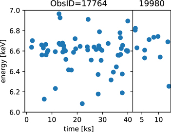
Figure 10. Arrival times of individual photons in the Fe feature for the two observations taken in 2017. Because of the limited energy resolution of the detector, we cannot say whether any individual photon is emitted in the continuum or in a line, but the figure shows that photons between 6.5 and 6.8 keV, which are likely to come from the Fe emission feature, are detected throughout the observation.
Download figure:
Standard image High-resolution imageFootnotes
- 8
- 9