Abstract
The proposition that life can spread from one planetary system to another (interstellar panspermia) has a long history, but this hypothesis is difficult to test through observations. We develop a mathematical model that takes parameters such as the microbial survival lifetime, the stellar velocity dispersion, and the dispersion of ejecta into account in order to assess the prospects for detecting interstellar panspermia. We show that the correlations between pairs of life-bearing planetary systems (embodied in the pair-distribution function from statistics) may serve as an effective diagnostic of interstellar panspermia, provided that the velocity dispersion of ejecta is greater than the stellar dispersion. We provide heuristic estimates of the model parameters for various astrophysical environments and conclude that open clusters and globular clusters appear to represent the best targets for assessing the viability of interstellar panspermia.
1. Introduction
The modern conception of “lithopanspermia,” i.e., the idea that life can travel across planetary systems carried by meteoroids and other minor bodies, dates back to at least the 19th century (Kamminga 1982); but it has regained serious consideration in scientific discussions (Melosh 1988; Wesson 2010; Wickramasinghe 2010). This revival was motivated by a number of developments. First, data concerning the resistance of radiation-tolerant organisms in deep space, as well as experimental tests of hypervelocity impacts, show that it is plausible that some organisms can survive the accidental transfer from an inhabited planet to another location (Horneck et al. 2010; Onofri et al. 2012; Merino et al. 2019). Second, there is now strong evidence that rock fragments have in fact been exchanged between nearby planets in the solar system (Nyquist et al. 2001) and it is conceivable that similar mechanisms can be even more efficient in more densely packed planetary systems, such as the TRAPPIST-1 system (Krijt et al. 2017; Lingam & Loeb 2017). Finally, the direct observation of at least two objects of interstellar origin transiting the solar system has confirmed that the exchange of material is possible even between different planetary systems (Meech et al. 2017; Guzik et al. 2020).
The actual feasibility of lithopanspermia on interstellar distances has been addressed in the past and shown to be achievable, at least in principle (Zubrin 2001; Napier 2004; Wallis & Wickramasinghe 2004; Ginsburg et al. 2018; Siraj & Loeb 2020), especially in crowded environments, such as in star-forming clusters (Adams & Spergel 2005; Valtonen et al. 2009; Belbruno et al. 2012) or in the Galactic bulge (Chen et al. 2018; Balbi et al. 2020). Furthermore, its probability can be significantly enhanced by interactions with binary systems (Lingam & Loeb 2018). Although the issue is still debated and, admittedly, rather speculative, there are strong theoretical motivations to explore how a viable lithopanspermia mechanism could impact the distribution of life in the Galaxy, particularly if compared to the case where life originates independently in separate locations.
There are at least two major implications that warrant a careful analysis of the problem (Balbi 2021). First, lithopanspermia may change the estimated extent of the Galactic Habitable Zone, since it can act as a compensating factor with respect to potentially catastrophic events that can eradicate life from planetary surfaces (Balbi et al. 2020). Second, it can alter the statistical impact and interpretation of future biosignature detections via surveys of nearby planetary systems as shown by Balbi & Grimaldi (2020).
Therefore, we argue it is timely to develop models that can shed some light on the consequences of interstellar lithopanspermia, assuming it is a practical mechanism. In this article, we present a theoretical treatment of the expected statistical distribution of inhabited planets in a lithopanspermia scenario, with a particular focus on its correlation properties. Our work generalizes and quantifies the prior analyses by Lin & Loeb (2015) and Lingam (2016a, 2016b), which dealt with this topic.
2. Formalism
To model the spreading of life over interstellar distances, we suppose that impacts of meteoroids and other minor celestial bodies on rocky planets collectively engender a steady ejection rate of matter escaping the gravitational pull of the host star. This assumption has been employed in several publications on interstellar lithopanspermia. Melosh (2003) predicted, for example, that ∼15 rocks of size >10 cm originating from impacts on inner planets exit the solar system each year on average. On the other hand, when it comes to micron-sized fragments, they are thought to be expelled at an average rate of ≳1014 per year (Napier 2004). While the ejection rate is likely to have been boosted during an epoch of intense bombardment as a result of the higher impact rates (Adams & Spergel 2005; Belbruno et al. 2012), our model does not necessitate knowledge of the exact value of this parameter, as long as it is not infinitesimally small.
A fraction of the rocks ejected from planets harboring a biosphere may encapsulate simple forms of life that, provided that they are appropriately shielded from UV and ionizing radiation as well as desiccation and other extremes, can possibly survive in space over timescales of millions of years (Mileikowsky et al. 2000; Lingam & Loeb 2021). On a related note, as per some (rather controversial) studies, Earth-based microbes might be capable of survival for intervals as high as ∼100 Myr under suitable conditions (Cano & Borucki 1995; Vreeland et al. 2000; Morono et al. 2020).
A world harboring a biosphere could thus be envisioned as being surrounded by a spherical region of radius R sparsely populated by life-bearing ejecta (Wallis & Wickramasinghe 2004). Under favorable circumstances, these objects could potentially seed life on an initially sterile planet located within such spheres of influence, each of which is termed a Lebenssphäre (life sphere). We roughly estimate the average radius of a Lebenssphäre by R = 〈vo 〉τo , where τo is the mean lifetime of the microbial populations encapsulated in the ejecta and 〈vo 〉 is the mean velocity of the objects in the local frame of the Lebenssphäre. By adopting a Maxwellian velocity distribution with dispersion σo , the average radius can be expressed as follows:

yielding, for example, R ≃ 50–100 ly in the event σo = 10–20 km s−1 and τo as large as 1 Myr. A sphere of influence of this size located in the solar neighborhood would contain ∼103–104 stars and a comparable number of rocky planets, while it would accommodate a number of stars up to four orders of magnitude greater if located in the Galactic bulge. We further note that a seeding sphere of ∼50 ly in radius is much smaller than most typical length scales in the Galaxy. This allows us to consider volume samples of the Galaxy of linear size larger than R but, at the same time, sufficiently small that the distribution of stars in the sample may be treated as homogeneous and isotropic.
If a planet to which life has been successfully transferred through lithopanspermia can sustain an enduring biosphere, it will after some time develop a new Lebenssphäre surrounding it, which will potentially seed life on other planets in turn. We make the ostensibly reasonable hypothesis that this mechanism engenders Lebenssphären with a constant birthrate per planet, denoted by τ−1, whereas Lebenssphären formed by spontaneous and independent abiogenesis events grow at a constant rate γ per unit volume. Furthermore, we assume that the proliferation of life-harboring planets is counterbalanced by random sterilizing events such as nearby supernovas or other cataclysms (Gowanlock & Morrison 2018), so that within a sample volume there exists a constant number density ρ of Lebenssphären formed around planets on which life arose spontaneously or by lithopanspermia. As shown in Appendix A, such steady-state regimes are reached as long as the inequality L/τ < 1 holds true, where L denotes the average persistence lifetime of a Lebenssphäre, consequently yielding ρ = γ L/(1 − τ/L).
In the following statistical analysis, it is mathematically convenient to first evaluate the static limit where all the stars in the sample have fixed positions that do not change over time. This is not a bad assumption as long as the stellar velocity dispersion is sufficiently low. The Lebenssphären, which we assume all possess the same mean radius R for simplicity, will therefore have their center at given immutable positions. The average number of the centers of Lebenssphären within a distance R from a randomly chosen seeding world is:

where g(r) represents the pair-distribution function defined in such a way that ρ2 g(r) leads to the probability distribution function associated with two Lebenssphäre centers being situated at a distance r from each other. If we suppose that life arose independently on different planetary systems (i.e., independent abiogenesis), the Lebenssphäre centers would be spatially uncorrelated, as schematically shown in Figure 1(a). In this case, it follows that g(r) = 1 and therefore

We now suppose that a panspermia mechanism along the lines described previously is able to spread life. In the static limit, a planet fertilized through panspermia (which in turn develops its own Lebenssphäre) must be located at a distance r ≤ R from the center of a Lebenssphäre, as illustrated in Figure 1(b). The coordination number N(R) must therefore be larger than its value in the absence of panspermia, Equation (3), because there now exists, within R, a higher probability of finding a planet to which life has been transferred:

where χ ≥ 1 accounts for the enhanced population of life-bearing planets located within R. We hereafter christen χ the panspermia amplification factor (PAF). Equation (4) simply states that, compared to the case of spontaneous and independent abiogenesis, the pair-distribution function is accordingly enhanced in the neighborhood of a seeding planet. We specify g(r) = χ for r ≤ R, which amounts to assuming that the probability of seeding a planet is uniform for r ≤ R. Although a more realistic ansatz is feasible, we wish to primarily explicate the qualitative features of this model.
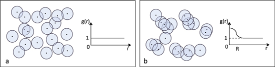
Figure 1. Schematic illustration of Lebenssphären (circles) centered around life-bearing planets (points). Case a: independent abiogenesis results in a uniform spatial distribution of Lebenssphären. Their centers are spatially uncorrelated and the pair-distribution function is g(r) = 1. Case b: when panspermia sets in and the stellar velocities are minimal, the Lebenssphären are aggregated in clusters formed by life-bearing planets at pair distances smaller than R. In this scenario, g(r) peaks at r ≲ R.
Download figure:
Standard image High-resolution imageAt greater distances, we expect the pair-distribution function to vary on a length scale of order ξ, eventually reaching the uniform limit g(r) = 1 for r ≫ ξ, where ξ measures the typical size of clusters formed by life-bearing planets at pair distances smaller than R. The spatial distribution of such “connected” planets is given by the so-called pair-connectedness function P(r), defined such that ρ2 P(r) gives the probability distribution function associated with finding two Lebenssphäre centers separated by a distance r and belonging to the same cluster (Torquato 2002). From this definition it follows that P(r) = g(r) for r ≤ R, while P(r) decays exponentially over distances larger than ξ, when no giant cluster of connected planets emerges. In the language of percolation theory, this regime amounts to being below the percolation threshold (Stauffer & Aharony 1994).
The above considerations suggest the following ansatz:

from which we recover the equality g(r) = χ ≥ 1 for r ≤ R, which we had posited earlier. To find g(r) for r > R we calculate P(r) by following standard techniques developed in continuum percolation theory and briefly described in Appendix B. Figure 2 depicts g(r) calculated for η = 0.4 and for values of the PAF ranging from χ = 1 (no panspermia) up to χ = 10, at which point the system reaches the percolation threshold ηc χ = 4 (Appendix B.2). Aside from the enhanced g(r) for r ≤ R, we see from Figure 2 that the higher is the PAF (i.e., larger χ), the greater is the distance above which g(r) → 1 is applicable.
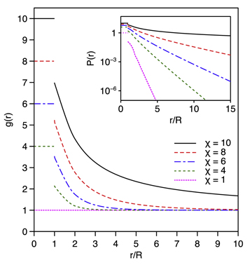
Figure 2. Pair-distribution function g(r) calculated in the static limit for η = 0.4 and different values of the panspermia intensity parameter χ. Inset: log-linear plot of the pair-connectedness function demonstrating that P(r) decays exponentially with r when the system is below the percolation threshold η χ = 4. At the critical point, P(r) ∝ 1/r.
Download figure:
Standard image High-resolution imageThis can be understood by noticing that the correlation length scales as ξ ∝ η χ/(1 − η χ); see Equation (B13) of Appendix B.3, which increases monotonically with χ and eventually diverges at the percolation threshold of η χ = 4. At this point, P(r), and therefore g(r) − 1 due to Equation (5), decays as a power law (inset of Figure 2). It is worth pointing out that our panspermia model predicts a critical density of percolation that is inversely proportional to χ—specifically, ηc = 4/χ as shown in Appendix B.2—meaning that a sufficiently high PAF is capable of inducing an entire sample-spanning transfer of life even if life-bearing planets are, overall, very rare.
The ansatz (5) is strictly applicable only to the subcritical regime wherein η < ηc . Once we exceed the percolation threshold, characterized by the formation of a giant cluster (Stauffer & Aharony 1994), we expect that the pair-distribution function generated by the panspermia process would gradually become less peaked as η increases beyond the percolation threshold, eventually tending toward g(r) = 1 for η ≫ 1/χ. In this limit, indeed, the Lebenssphären would essentially cover the entire sample volume in a uniform fashion.
We will now extend the static panspermia mechanism discussed above to the more realistic case in which stars hosting planetary systems have nonzero relative velocities. Intuitively, even if the static panspermia model may evince pronounced spatial correlations, we would expect them to be nevertheless weakened by the accompanying stellar motion. To explore this effect, we note that for Lebenssphären that are generated via panspermia at a constant rate τ−1, the position of a newly formed Lebenssphäre relative to that of the seeding planet will be translated by ∼ v τ, where v is the relative velocity of the two planetary systems. We capture this effect by rewriting the ansatz (5) as:

where f( v ) is the distribution function of the relative velocities. Assuming that in the local frame of the sample volume the stars move in random directions with velocities obeying a Maxwell distribution with dispersion σs , Equation (6) can be recast in the following form:

where  measures the dispersion of the relative distance between two centers of Lebenssphären. Clearly, for σr
→ 0 we recover the ansatz (5), while for σr
≫ R the pair-distribution of the Lebenssphäre centers reaches the uniform limit as
measures the dispersion of the relative distance between two centers of Lebenssphären. Clearly, for σr
→ 0 we recover the ansatz (5), while for σr
≫ R the pair-distribution of the Lebenssphäre centers reaches the uniform limit as  .
.
We show the crossover from the correlated to the uncorrelated regime in Figure 3, where we report the numerical calculations of g(r) obtained by self-consistently solving Equation (7) and the integral equation of P(r) (Appendix B.1). The enhancement of g(r) for r ≤ R is rapidly weakened as σr increases and, simultaneously, the correlation length declines toward the uncorrelated limit (inset of Figure 3). In fact, even for σr /R ≈ 1 the pair-distribution function is essentially indistinguishable from that of a fully uncorrelated system; the latter refers to the case with χ = 1 in Figure 2.
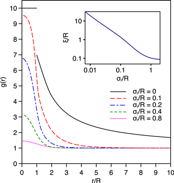
Figure 3. Pair-distribution function g(r) calculated for η = 0.4, χ = 10 in the case of nonzero stellar velocity dispersion σs
. The parameter  measures the dispersion of the relative separation of Lebenssphäre centers. Note that σr
= 0 corresponds to the static limit. As σr
increases, the discontinuity of g(r) at r = R is smeared out and the peak at r ≲ R is weakened. For σr
≳ R the pair-distribution function becomes flat as in the uncorrelated case. Inset: correlation length ξ plotted as a function of σr
/R.
measures the dispersion of the relative separation of Lebenssphäre centers. Note that σr
= 0 corresponds to the static limit. As σr
increases, the discontinuity of g(r) at r = R is smeared out and the peak at r ≲ R is weakened. For σr
≳ R the pair-distribution function becomes flat as in the uncorrelated case. Inset: correlation length ξ plotted as a function of σr
/R.
Download figure:
Standard image High-resolution imageFor σr /R ≳ 1, therefore, the Lebenssphäre centers are uniformly distributed, thereby hindering our ability to infer any information about the extent and intensity of panspermia events if one were to simply measure the distribution of life-bearing planets in a given sample volume through an appropriate survey.
3. Discussion
It is now instructive to carry out some fiducial estimates for select astrophysical systems and consequently assess the efficacy of panspermia. Of the various parameters at play, one of the most ambiguous among them is τ, which is the time elapsed from a seeding event to the formation of a Lebenssphäre of radius R, owing to which it cannot be smaller than τo . If we suppose that life could germinate quickly after the seeding event and form a biosphere, given habitable conditions, it is conceivable that τ is of the same order as τo , owing to which we will employ the condition τ ≳ τo .
One other crucial variable is ρ because it regulates η, as seen from Equation (3). Given that ρ is the number density of Lebenssphären, this is not an easy quantity to gauge since it requires us to know the fraction of planetary systems with habitable worlds on which life blossomed into a biosphere (ζ⋆). In essence, therefore, it corresponds to two weakly constrained factors in the Drake equation (Drake 1965). As per our postulate, we have ρ = ζ⋆ ρ⋆, where ρ⋆ is the stellar density. In the static limit, we have shown that the percolation threshold is ηc = 4/χ in Appendix B.2, which implies that ηc < 4 because χ > 1 by construction. It is therefore feasible to determine an upper bound on ζ⋆ (denoted by ζc ) in order for η to stay below the percolation threshold and in the subcritical regime from Equation (3) as follows:

If ρ⋆ and/or R are sufficiently small, then ζc > 1 is mathematically possible; but not physically realizable because we have defined ζ such that it is smaller than unity. Hence, environments with ζc < 1 are liable to always exist in the subcritical regime with η < ηc . Estimating the required value of ζc is helpful because it functions as a heuristic signpost for determining whether we are below or above the percolation threshold. In the latter scenario, as explained in Section 2, the panspermia correlations manifested in the pair-distribution function could become indistinguishable if η is high.
At this juncture, we emphasize that some of our ensuing results are not sensitive to η. For instance, the crucial ratio of σr /R is expressible as

which implies that a sufficient condition for σr /R ≳ 1 to hold true is σs ≳ 1.13 σo . This relation follows after utilizing τ ≳ τo from the preceding paragraph. Thus, broadly speaking, if the stellar velocity dispersion is higher than that of the ejecta, the panspermia correlations are effectively washed out. If the opposite is true, then the correlated regime might be manifested, enabling us to discern panspermia through observations; but only provided that τ is roughly comparable to τo .
In what follows, we will suppose that the characteristic dispersion of ejecta from planetary systems is σo ∼ 10 km s−1, which is close to the mean value of 6.2 ± 2.7 km s−1 for ejection speeds estimated in Adams & Spergel (2005). However, it should be noted that a small fraction of ejecta may have speeds of order 0.1 km s−1 (Belbruno et al. 2012). The estimate for τo is not well understood, since it depends on the size of the object among other factors; but survival timescales of ≳1 Myr are possible for microbial populations in ejecta with sizes of ≳1 m (Mileikowsky et al. 2000; Valtonen et al. 2009; Lingam & Loeb 2021) and intervals of ∼10–100 Myr are not impossible (Cano & Borucki 1995; Morono et al. 2020). We will therefore specify τ0 ∼ 1 Myr hereafter. Although we adopt this fiducial value, our results regarding the viability of detecting panspermia are sensitive to the ratio τ/τo , as seen Equation (9), and are consequently not directly dependent on the magnitude of τo .
We have presented heuristic estimates for the salient parameters of our model in Table 1. As τ is subject to significant uncertainty, we have considered the limiting case of τ ∼ τo herein and adopted the values delineated in the prior discussion. There are two broad inferences that can be drawn from this table.
- 1.We find that ζc ≪ 1 is valid for all astrophysical environments except the Galactic halo. Thus, insofar as the static limit is concerned, the subcritical regime (with η below the percolation threshold) is feasible when the density of Lebenssphären is very low. To put it differently, if only a very small fraction of planetary systems develop Lebenssphären in these astrophysical settings, the subcritical regime is valid.
- 2.It was argued earlier that panspermia correlations are discernible only when σr /R ≲ 1. We notice from Table 1 that this criterion is comfortably satisfied only in the case of open stellar clusters, although globular clusters and the solar neighborhood are not far removed from this desired limit.
Table 1. Heuristic Estimates of Model Parameters for various Astrophysical Environments
| System | σo | σs | τo | τ | R | σr | σr /R | ρ⋆ | ζc |
|---|---|---|---|---|---|---|---|---|---|
| Solar neighborhood | 10 | 20 | 1 | 1 | 53 | 94 | 1.8 | 2.9 × 10⁻³ | 2.2 × 10⁻³ |
| Globular clusters | 10 | 5 | 1 | 1 | 53 | 23.5 | 0.4 | 2.9 | 2.2 × 10⁻⁶ |
| Open clusters | 10 | 1 | 1 | 1 | 53 | 4.7 | 9 × 10⁻² | 0.3 | 2.2 × 10⁻⁵ |
| Galactic bulge | 10 | 100 | 1 | 1 | 53 | 470 | 8.9 | 0.3 | 2.2 × 10⁻⁵ |
| Galactic halo | 10 | 150 | 1 | 1 | 53 | 705 | 13.3 | 1.4 × 10⁻⁵ | 4.6 × 10⁻¹ |
Note. σo and σs are expressed in units of km s−1, R and σr in units of light years (ly), τ and τ0 in units of Myr, and ρ⋆ in units of stars per cubic ly. The parameters for the above systems were chosen based on the following references: (i) solar neighborhood (Holmberg et al. 2009); (ii) globular clusters (Baumgardt & Hilker 2018); (iii) open clusters (Valtonen et al. 2009; Foster et al. 2015); (iv) Galactic bulge (Zhu et al. 2017; Balbi et al. 2020); and (v) Galactic halo (Helmi 2008).
Download table as: ASCIITypeset image
4. Conclusions
We presented the results of a mathematical model describing the dissemination of life over interstellar distances through lithopanspermia. The model depends on a number of parameters that are known to varying degrees of accuracy, but all of them can be empirically constrained in principle.
We have focused on the predicted correlation properties of life-bearing planetary systems. Our calculations show that an active panspermia process could lead to a distinct amplification of the population of life-bearing planets within a certain characteristic distance compared to the case of independent abiogenesis. This correlation distance is sensitive to the details of the lithopanspermia mechanism and is therefore capable of serving as an observational diagnostic to constrain various scenarios. However, we also demonstrated that the correlations can become attenuated, or even nullified altogether, depending on the astrophysical environment under investigation. As this attenuation is related to dynamical parameters, in particular to the velocity dispersion of stellar systems, it may be predicted to an extent in specific settings.
Hence, based on our formalism, we found that stellar clusters are more promising insofar as detecting the instantiation of panspermia is concerned, although it might still be discernible in our solar neighborhood. On the other hand, crowded environments endowed with high stellar dispersions, such as the galactic bulge, could be so effective at spreading life through lithopanspermia that they are essentially indistinguishable from the case with minimal panspermia and a high-abiogenesis rate. In other words, the correlations would be washed out.
Given our findings, at least two further directions are worthy of pursuit in future investigations. First, our work can be expanded and refined by carrying out detailed numerical simulations and proceeding beyond some of the simplifying assumptions adopted, most notably the criterion of being below the percolation limit. Such numerical simulations are expected to yield further insights concerning the feasibility of distinguishing between independent abiogenesis and panspermia in a given astrophysical system and what number of inhabited worlds need to be detected toward this end. From an observational standpoint, it has been suggested that confirming panspermia at 5σ confidence requires the sampling of >25 life-bearing worlds in the optimal scenario (Lin & Loeb 2015).
It is necessary, in the same vein, to investigate the relative weights of proliferation versus sterilization as these process govern the prevalence of life in planetary systems, as shown in Appendix A. Second, as a separate line of inquiry, experimental studies of the viability of panspermia would pave the way for estimating some of the parameters involved (e.g., survival time of extremophile populations in space), consequently evaluating the prospects of detecting life on other planets and gauging the feasibility of interstellar panspermia.
The authors thank the reviewer for the constructive feedback, which was helpful for improving the paper. A.B. was partially funded by the Italian Space Agency through the Life in Space project (ASI N. 2019-3-U.0) and by grant No. FQXi-MGA-1801 and FQXi-MGB-1924 from the Foundational Questions Institute and Fetzer Franklin Fund, a donor advised fund of Silicon Valley Community Foundation.
Appendix A: Rate Equation for the Density of Lebenssphären
We make the assumption that within a given volume sample there is a number density ρ0 of planets on which life arose spontaneously and independently. If we denote by γ the rate of formation per unit volume of Lebenssphären created by spontaneous abiogenesis and L embodies their typical lifetime, the rate equation for ρ0 reads

In the presence of panspermia, however, there will be an additional number density ρp contribution arising because life has been transferred and new Lebenssphären have been accordingly formed. Given that life can be transferred from planets on which life arose spontaneously or via prior panspermia events, the corresponding rate equation is

where τ−1 is the formation rate of Lebenssphären (per planet) due to panspermia and in the last term we have presumed that sterilizing events affect ρp to effectively the same degree as ρ0. The rate equation for ρ = ρ0 + ρp is therefore given by

The above differential equation admits two types of solutions depending on whether the formation rate of Lebenssphären is greater or smaller than the rate of sterilizing events. The solution for L/τ > 1 gives rise to a number density of life-harboring planets that increases exponentially with time. The special limit of L/τ = 1 would result in the number density growing linearly with time. In these cases, the rate of panspermia events is such that all habitable planets within the sample volume eventually develop a biosphere, thence leading to a spatially uniform distribution of Lebenssphären. On the contrary, when it comes to L/τ < 1, the solution of Equation (A3) for t ≫ L/(1 − L/τ) reaches the steady-state regime in which ρ is finite and expressible as

It is in such a regime of dynamical equilibrium that the spatial distributions of Lebenssphären is anticipated to show nontrivial correlations.
Appendix B: Connectedness Model of Panspermia
B.1. Pair-connectedness Function
In our model of panspermia, we define two planets as being “connected” if their relative distance is smaller than R; namely, the radius of their Lebenssphären. In this fashion, the pair-distribution function can be decomposed into a “connected” part and a “disconnected” part: g(r) = P(r) + B(r). Here, P(r) is the pair-connectedness function associated with finding two Lebenssphären, with centers separated by a distance r within the same cluster. B(r) is the pair-blocking function associated with finding two Lebenssphären at distance r not belonging to the same cluster (Torquato 2002). From these definitions it follows that P(r ≤ R) = g(r) and B(r ≤ R) = 0. It is worth pointing out that the ansatz (5) adopted for the static limit is actually an approximation for B(r); it can be obtained from g(r) = P(r) + B(r) by replacing B(r) with 1 − P(r)/χ, which satisfies the condition B(r ≤ R) = 0. Since the pair-connectedness function fully defines our model g(r), Equation (5), we exploit the standard integral equation method of continuum percolation theory to find P(r) via the solution of the Ornstein–Zernike relation (Chiew & Glandt 1983; DeSimone et al. 1986):

where ρ is the number density of the Lebenssphären and D(r) is the direct-connectedness function that is applicable to Lebenssphären that are directly connected (i.e., the relative distance between their centers is r ≤ R). Equation (B1) is solvable by imposing a suitable closure relation. Here, we use D(r) = 0 for r > R, which is basically the well-known Percus–Yevick closure relation utilized in the theory of liquids (Hansen & McDonald 2006). We implement the so-called Baxter factorization to solve Equation (B1) under the condition

This amounts to decoupling P(r) from D(r) by introducing a new function q(r), having the property q(r) = 0 for r < 0 and r > R, which is related to the pair-connectedness and direct-connectedness functions by:

where  and
and  are the Fourier transforms of P(r) and D(r), respectively, and

The factorization enables us to express P(r) in terms of q(r) (see Hansen & McDonald 2006 for a thorough derivation):

where  . The function q(r) can be found by solving Equation (B5) for 0 < r < R, since in this range P(r) = g(r):

In the static limit of our panspermia model, the pair-distribution function for 0 < r < R is simply g(r) = χ, so that the solution Equation (B6) is of the form  . Given the boundary condition q(R) = 0, we find therefore:

Substitution of this result into Equation (B6) allows us to find the coefficients α and β:

where  . At this point, P(r) can be calculated by numerically solving Equation (B5) in the range r > R.
When we consider the effects of the stellar velocities, we follow essentially the same steps of the static case with the important difference that now g(r) and P(r) must be calculated self-consistently. In practice, we first integrate numerically Equation (7) using the pair-connectedness function P(r) calculated for the static limit as described above. The resulting g(r) is inserted into Equation (B6) and the integro-differential equation for q(r) is solved numerically. Next, P(r) is calculated by solving Equation (B5) across the entire range of r and inserted back into Equation (7). We repeat this procedure until convergence is reached.
B.2. Percolation Threshold
It should be noted that the Ornstein–Zernike relation (B1) applies below the percolation threshold where no giant cluster of connected centers of Lebenssphären exists. The percolation threshold is the point at which the mean cluster size

diverges. Using Equations (B3) and (B4), S can be expressed in terms of the function q(r):

In the static limit, S can be calculated analytically using Equations (B7) and (B8), yielding  , which diverges at the critical point η
χ = 4.
, which diverges at the critical point η
χ = 4.
B.3. Correlation Length
We calculate the correlation length ξ by solving Equation (B5) for r ≫ R. Letting f(r) = rP(r) we can recast (B5) as a differential equation for f(r):
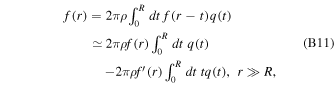
where we have used  for t ≤ R ≪ r. It is straightforward to solve Equation (B11) to find
  , where the correlation length is given by:

In the static limit, ξ can be calculated analytically by inserting Equations (B7) and (B8) into the above expression:

Note that the percolation length also diverges at the percolation threshold of η χ = 4 derived in Appendix B.2, which is a classic feature of percolation theory (Stauffer & Aharony 1994).
When the stellar motion is taken into consideration, the resulting correlation length is readily obtained by inserting into Equation (B12) the function q(r), which is calculated numerically as described in Appendix B.1.