Abstract
Near-Earth Objects (NEOs) are a transient population of small bodies with orbits near or in the terrestrial planet region. They represent a mid-stage in the dynamical cycle of asteroids and comets, which starts with their removal from the respective source regions—the main belt and trans-Neptunian scattered disk—and ends as bodies impact planets, disintegrate near the Sun, or are ejected from the solar system. Here we develop a new orbital model of NEOs by numerically integrating asteroid orbits from main-belt sources and calibrating the results on observations of the Catalina Sky Survey. The results imply a size-dependent sampling of the main belt with the ν6 and 3:1 resonances producing ≃30% of NEOs with absolute magnitudes H = 15 and ≃80% of NEOs with H = 25. Hence, the large and small NEOs have different orbital distributions. The inferred flux of H < 18 bodies into the 3:1 resonance can be sustained only if the main-belt asteroids near the resonance drift toward the resonance at the maximal Yarkovsky rate (≃2 × 10⁻⁴ au Myr−1 for diameter D = 1 km and semimajor axis a = 2.5 au). This implies obliquities θ ≃ 0° for a < 2.5 au and θ ≃ 180° for a > 2.5 au, both in the immediate neighborhood of the resonance (the same applies to other resonances as well). We confirm the size-dependent disruption of asteroids near the Sun found in previous studies. An interested researcher can use the publicly available NEOMOD Simulator to generate user-defined samples of NEOs from our model.
Original content from this work may be used under the terms of the Creative Commons Attribution 4.0 licence. Any further distribution of this work must maintain attribution to the author(s) and the title of the work, journal citation and DOI.
1. Introduction
NEOs are asteroids and comets whose orbital perihelion distance is q < 1.3 au. Asteroids, which represent the great majority of NEOs on short-period orbits, are the main focus here, but we also include comets with a < 4.2 au. The goal is to develop an accurate model of the orbital and absolute magnitude distribution of NEOs that can be used to understand the observational incompleteness, design search strategies, and evaluate the impact risk. We aim at setting up a flexible scheme that can easily be updated when new observational data become available (from the Vera C. Rubin Observatory, NEO Surveyor, etc.).
We closely follow the methodology developed in previous studies (Bottke et al. 2002; Granvik et al. 2018; also see Greenstreet et al. 2012), and attempt to improve it whenever possible. This does not always mean that a new level of realism/complexity is added to the model. For example, Granvik et al. (2018) defined various NEO sources from numerical integrations where main-belt asteroids were drifted into resonances (Granvik et al. 2017). This is arguably a more realistic approach than simply placing test bodies into source resonances (Bottke et al. 2002). Here we opt for the latter method because it is conceptually simple and easy to modify. We verify, when possible (e.g., Section 9), that the main results are not affected by this simplifying assumption.
We develop a new method to accurately calculate biases of NEO surveys and apply it to the Catalina Sky Survey (CSS). The MultiNest code, a Bayesian inference tool designed to efficiently search for solutions in high-dimensional parameter space (Feroz & Hobson 2008; Feroz et al. 2009), is used to optimize the model fit to CSS detections. We adopt cubic splines to characterize the magnitude distribution of the NEO population. Cubic splines are flexible and can be modified to consider a broader absolute magnitude range and/or improve the model accuracy. We use a large number of main-belt asteroids in each source (105), which allows us to accurately estimate the impact fluxes on the terrestrial planets. Our model self-consistently accounts for the NEO disruption at small perihelion distances (Granvik et al. 2016).
This article is structured as follows. We define NEO sources (Section 2), carry out N-body integrations to determine the orbital distribution of NEOs from each source (Section 3), and combine different sources together by calibrating their contributions from CSS (Section 4). The model optimization with MultiNest is described in Section 5. The final model, hereafter NEOMOD, synthesizes our current knowledge of the orbital and absolute magnitude distribution of NEOs (Section 6). It can readily be upgraded as new NEO observations become available. We provide the NEOMOD Simulator 13 —an easy-to-operate code that can be used to generate user-defined samples of model NEOs. Planetary impacts are discussed in Section 7. Section 8 considers several modifications of our base model. In Section 9, we drift main-belt asteroids toward source resonances to test whether the flux of bodies into resonances is consistent with the results inferred from the NEO modeling.
2. Source Populations
To set up the initial orbits of main-belt asteroids in various NEO sources, we made use of the astorb.dat catalog from the Lowell Observatory (Moskovitz et al. 2022). 14 As of early 2022, the astorb.dat catalog contained nearly 1.2 × 10⁶ entries, the great majority of which were main-belt asteroids. For each source, we inspected the known asteroid population near the source location to define the initial distribution of orbits for our numerical integrations. We illustrate the method for the 3:1 resonance at a = 2.5 au, which is a notable source of NEOs identified by many previous studies (e.g., Wisdom 1985; Gladman et al. 1997; Bottke et al. 2002; Morbidelli & Vokrouhlický 2003; Greenstreet et al. 2012; Granvik et al. 2018); other resonances are discussed later on.
In Figure 1, the 3:1 resonance appears as a V-shaped gap—this is the place where Jupiter’s gravitational perturbations build up to boost the object’s orbital eccentricity (Wisdom 1982). The borders of the gap are approximately a1 = 2.5 − (0.02/0.35)e au and a2 = 2.5 + (0.02/0.35)e au, where e is the orbital eccentricity. The 3:1 source population is represented in this work by 105 test bodies (not shown in Figure 1) placed within the gap borders. In reality, the main-belt asteroids evolve into the resonance by the Yarkovsky thermal effect (Vokrouhlický et al. 2015), but this is not considered here. In Section 9, we drift asteroids into resonances and find that the orbital distribution of NEOs is insensitive to how the resonant sources are populated (e.g., to the initial resonant amplitude distribution). One needs to be careful, however, with the eccentricity and inclination distributions of source orbits (Bottke et al. 2002; Granvik et al. 2018).
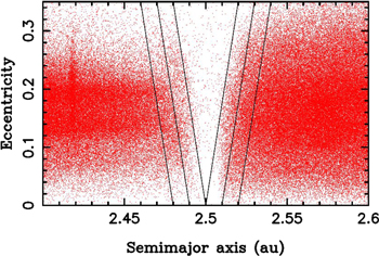
Figure 1. The orbital distribution of main-belt asteroids (red dots) near the 3:1 resonance with Jupiter. The inner V-shaped region approximates the dynamically unstable domain where test bodies representing the 3:1 source were placed. The main-belt asteroids with orbits in the two outer strips, 2.48 < a < 2.49 au and 2.51 < a < 2.52 au for e = 0 and diagonally extending to e > 0, were used to set up the eccentricity and inclination distributions of test bodies.
Download figure:
Standard image High-resolution imageWe define two strips in (a, e), one on the left side and one on the right side of the 3:1 resonance (Figure 1), and use the known asteroids in these strips to set up the eccentricity and inclination distributions for the 3:1 source. The idea is that bodies entering the 3:1 resonance should have e and i distributions similar to bodies in the strips. For 3:1, the left strip is defined as a > 2.48 − (0.02/0.35)e au and a < 2.49 − (0.02/0.35)e au, and the right strip is defined as a > 2.51 + (0.02/0.35)e au and a < 2.52 + (0.02/0.35)e au. The Mars-crossing orbits are avoided. Both strips have a fixed (e-independent) width to assure even sampling. To limit problems with the observational incompleteness, which may unevenly affect asteroid populations with different e/i, we only consider bodies with absolute magnitudes H < 18 (cuts with H < 15, H < 16 or H < 17 produce similar results). This means that the orbital distribution within a single source is size independent. The size dependence appears in our NEO model due to the size-dependent weights of different sources (Section 5.1) and the size-dependent disruption (Section 5.3).
The orbital distribution of known asteroids in the strips is parameterized by analytic functions, which are then used to generate synthetic bodies. This two-step procedure is useful to leave the record of the adopted distributions (Table 1). Specifically, we experimented with the single Gaussian, double Gaussian, Rayleigh, and Maxwell–Boltzmann distributions. For the 3:1 resonance, the eccentricity distribution is well approximated by a single Gaussian with a mean μ = 0.145 and width σ = 0.067, and an inclination distribution with a double Gaussian with μ1 = 47, σ1 = 2
7, μ2 = 13
5, and σ2 = 2
5, where the first Gaussian is given a 2.5 times greater weight than the second one (i.e., the weight ratio w1/w2 = 2.5; Figure 2).
15
Table 1 reports parameters of the adopted analytic distributions for all sources.
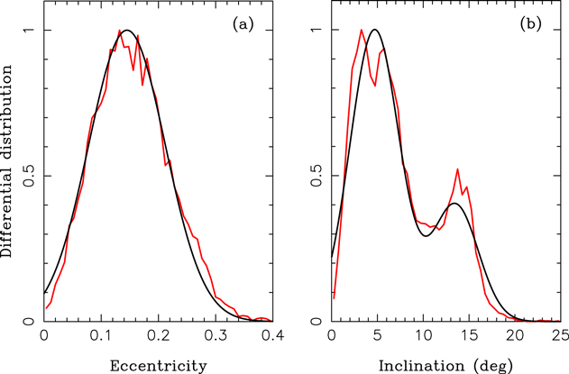
Figure 2. The eccentricity (panel (a)) and inclination (panel (b)) distributions of bodies placed in the 3:1 resonance with Jupiter. The red lines are the actual distributions of main-belt asteroids near the 3:1 resonance. The black lines are the analytic approximation of these distributions described in the main text.
Download figure:
Standard image High-resolution imageTable 1. Eccentricity and Inclination Distributions Adopted in This Work for Different Sources
| Source | μe | σe | μ1 | σ1 | μ2 | σ2 | w1/w2 |
|---|---|---|---|---|---|---|---|
| (or γe ) | (°) | (°) | (°) | (°) | |||
| ν6 | 0.16 | 0.067 | 5.5 | 2.3 | 15.0 | 3.0 | 10 |
| 3:1 | 0.145 | 0.067 | 4.7 | 2.7 | 13.5 | 2.5 | 2.5 |
| 5:2 | (0.1) | ⋯ | 5.5 | 3.0 | 13.5 | 4.0 | 3.3 |
| 7:3 | (0.085) | ⋯ | 2.7 | 1.3 | 10.5 | 2.2 | 0.65 |
| 8:3 | (0.1) | ⋯ | 5.3 | 2.0 | 13.0 | 2.3 | 1.4 |
| 9:4 | (0.09) | ⋯ | 2.0 | 2.0 | 10.5 | 3.3 | 0.3 |
| 11:5 | (0.11) | ⋯ | 10.0 | 1.0 | 10.0 | 6.0 | 1.0 |
| 2:1 | (0.12) | ⋯ | 26.0 | 2.0 | 11.0 | 6.0 | 0.55 |
Note. The columns are: (1) source ID, (2) the mean of the Gaussian distribution (μe ) or the scale parameter of the Rayleigh distribution (γe , values in parentheses) in e, (3) the standard deviation of the Gaussian distribution in e (σe ), (4)–(5) the mean and standard deviation of the first Gaussian term in i (μ1 and σ1), (6)–(7) the mean and standard deviation of the second Gaussian term in i (μ2 and σ2), and (8) the weight ratio of the two terms (w1/w2).
Download table as: ASCIITypeset image
For each draw of e and i, the semimajor axis is assigned randomly between a1 and a2. The perihelion (ϖ) and nodal (Ω) longitudes are drawn from a uniformly random distribution between 0 and 2π radians. The mean longitude λ is chosen such that θ3:1 = 3λJ
− λ − 2ϖ = π, where θ3:1 is the resonant angle of the 3:1 resonance, and λJ
is the mean longitude of Jupiter at the reference epoch (λJ = 34368 for MJD =2459600.5). With this choice, the initial resonant amplitude is simply Δa = ∣a − 2.5 au∣, and we can therefore easily check if different amplitudes would yield differing orbital distributions of NEOs (they do not; see Section 9 for additional tests). This completes the description for the 3:1 resonance.
We followed the same procedure for the 5:2, 7:3, 8:3, 9:4, 11:5, and 2:1 resonances with Jupiter, all of which can potentially be important sources of NEOs. In the preliminary tests, we also included the 7:2 resonance with Jupiter, and the 4:7 and 1:2 resonances with Mars. These resonances were tested to establish the importance of the “forest” of weak resonances in the inner main belt. Whereas these individual resonances are likely to be important for the NEO delivery, especially for large asteroids (Migliorini et al. 1998), we found that several trees cannot account for a forest. We thus followed the method described in Migliorini et al. (1998) to model all weak resonances (also see Bottke et al. 2002). Specifically, we extracted all known asteroids from the astorb.dat catalog with q > 1.66 au (i.e., no Mars crossers), 2.1 < a < 2.5 au, i < 18°, and H < 18 (163,971 bodies in total), and reduced that sample—by random selection—down to 105 orbits that define our “inner-belt” source. While it is not ideal to combine two different methods—one that places synthetic bodies into strong resonances (see above for 3:1) and one based on real main-belt asteroids (here for the inner belt)—we believe that this is the best practical approach to the problem at hand. The same method was used for the Hungaria (q > 1.66 au, a < 2.05 au, i > 15°) and Phocaea (q > 1.66 au, 2.1 < a < 2.5 au, 18° < i < 30°) asteroids. The known populations of Hungarias and Phocaeas were cloned 4 and 13 times, respectively, to obtain 105 source orbits for each. 16
The ν6 resonance, which lies at the inner edge of the asteroid belt, requires a special treatment. We place orbits in the strongly unstable part of the ν6 resonance where bodies are expected to evolve onto NEO orbits in <10 Myr (Morbidelli & Gladman 1998). The left and right borders of the ν6 source region in (a, i) are defined here as a1 = 2.062 + 0.00057 i2.3 au and a2 = a1 + 0.04 − 0.002 i au, with i in degrees. To define the initial e and i distributions in the ν6 resonance, we consider the distribution of real asteroids in the strip a > 2.12 + 0.00057 i2.3 au and a < 2.18 + 0.00057 i2.3 au, with i in degrees. The eccentricity distribution of bodies in the strip can be approximated by a single Gaussian with mean μ = 0.16 and width σ = 0.067, and an inclination distribution with a double Gaussian with μ1 = 55, σ1 = 2
3, μ2 = 15°, and σ2 = 3
0, and w1/w2 = 10 (Table 1). The mean and nodal longitudes are uniformly distributed between 0 and 2π radians. We set ϖ = ϖS, where ϖS is the perihelion longitude of Saturn at the reference epoch (ϖS = 88
98 for MJD =2459600.5). For each draw, the initial semimajor axis is randomly placed between a1 and a2 defined above.
Nesvorný et al. (2017) developed a dynamical model for Jupiter-family comets (JFCs). In brief, the model accounted for galactic tides, passing stars, and different fading laws. They followed 106 bodies from the primordial trans-Neptunian disk, included the effects of Neptune’s early migration, and showed that the simulations reasonably well reproduced the observed structure of the Kuiper Belt, including the trans-Neptunian scattered disk, which is the main source of JFCs. The orbital distribution and number of JFCs produced in the model were calibrated to the known population of active comets. We refer the reader to Nesvorný et al. (2017) for further details.
Here we use the model from Nesvorný et al. (2017) to set up the orbital distribution of comets in the NEO region. The comet production simulations from Nesvorný et al. (2017) were repeated to have better statistics for q < 1.3 au. Specifically, every body that evolved from the scattered disk to q < 23 au was cloned 100 times, and the code recorded all orbits with q < 1.3 au and a < 4.5 au (with a 100 yr cadence). This data represents our model for cometary NEOs. The model includes the population of long-period comets but does not account for the long-period comet fading (Vokrouhlický et al. 2019). Note that the current orbital distribution of JFCs is largely independent of details of the early evolution of the solar system. We thus do not need to investigate different cases considered in Nesvorný et al. (2017).
In summary, we have 12 sources in total: eight resonances (ν6, 3:1, 5:2, 7:3, 8:3, 9:4, 11:5, and 2:1), the forest of weak resonances in the inner belt, two high-inclination sources (Hungarias and Phocaeas), and comets.
3. Orbital Integrations and Binning
The orbital elements of eight planets (Mercury to Neptune) were obtained from NASA/JPL Horizons for the reference epoch (MJD = 2459600.5). We used the Swift rmvs4 N-body integrator (Levison & Duncan 1994) to follow the orbital evolution of planets and test bodies (105 per source). The integrations were performed with a short time step (12 hr). 17 For each source, we used 2000 Ivy Bridge cores of the NASA Pleiades Supercomputer, with each core following eight planets and 50 test bodies. The simulation set represented ∼10 million CPU hours in total. A test body was removed from the integration when it impacted the Sun, one of the planets, or was ejected from the solar system. All integrations were first run to t = 100 Myr. The test bodies that had NEO orbits (q < 1.3 au) at t = 100 Myr were collected, and their integration was continued to t = 500 Myr. We tested the contribution of long-lived NEOs for t > 500 Myr and found it insignificant.
The orbits of model NEOs were recorded with a 1000 yr cadence. This is good enough—with the large number of test bodies per source—to faithfully represent the orbital distribution from each source. For the ν6 and 3:1 resonances, we also tested the high-cadence sampling, with the orbits being recorded every 100 yr, and verified that the results were practically the same. The high-cadence sampling, however, generated data files that were too large to be routinely manageable with our computer resources (hundreds of gigabytes per source).
The integration output was used to define the binned orbital distribution of NEOs from each source j, dpj (a, e, i) = pj (a, e, i) da de di. We tested different bin sizes. On one hand, one wishes to represent the smooth orbital distribution as accurately as possible, without discontinuities. On the other hand, the MultiNest fits become CPU expensive if too many bins are considered. After experimenting with the bin size, we adopted the original binning from Granvik et al. (2018) for the MultiNest runs and used four times finer binning for plots (Figure 3). Table 2 reports the number of bins for the MultiNest runs and the range of orbital parameters covered by binning. 18
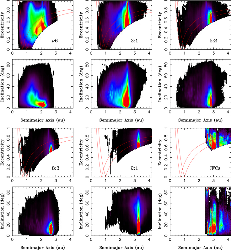
Figure 3. The projected PDFs of model NEO orbits for different sources (projected pj (a, e, i)): ν6, 3:1, 5:2, 8:3, 2:1 and JFCs (from top left to bottom right). Higher values are shown by brighter colors. For reference, the red lines show orbits with q = aEarth, Q = aEarth, q = aVenus, and Q = aVenus, where Q = a(1 + e) is the aphelion distance, aEarth = 1.0 au and aVenus = 0.72 au.
Download figure:
Standard image High-resolution imageTable 2. Orbit and Absolute Magnitude Binning Used in This Work
| Min | Max | Nbin | Δ | |
|---|---|---|---|---|
| a | 0 | 4.2 au | 42 | 0.1 au |
| e | 0 | 1 | 20 | 0.05 |
| i | 0 | 88° | 22 | 4° |
| H | 15 | 25 | 40 | 0.25 |
Note. The columns are: the (1) model variable, (2)–(3) minimum and maximum values considered here, (4) number of bins (Nbin), and (5) bin size (Δ).
Download table as: ASCIITypeset image
For each source, the orbital distribution was normalized to one NEO,

effectively representing the binned orbital probability density function (PDF). We used the orbital range a < 4.2 au, q < 1.3 au, e < 1 and i < 90°, hereafter the NEO model domain, because this is where all NEOs detected by CSS reside (Section 4; except for (343158) Marsyas with i = 154°). The model can be easily extended to include retrograde orbits. As the binning is done only in a, e, and i, the model ignores any possible correlations with the orbital angles (nodal, perihelion, and mean longitudes). Some correlations would arise due to orbital resonances with planets (JeongAhn & Malhotra 2014), but we do not investigate this issue here.
Given the vast number of bodies released from each source, the N-body integrator records a large number of planetary impacts. We record all impacts, including Mars impacts from impactors with q > 1.3 au (not NEOs), and use this information to compute the impact flux from each source. When the source-specific impact fluxes are properly weighted by accounting for the size-dependent sampling of sources (Section 5.1), we obtain an accurate record of NEO impacts on the planets (Mercury, Venus, Earth, and Mars). These results are discussed in Section 7.
4. Catalina Sky Survey
4.1. Observations
The Mt. Lemmon (IAU code G96) and Catalina (703) telescopes of CSS (Christensen et al. 2012) produced nearly 22,000 NEO detections and redetections during the 8 yr long period from 2005–2012. The two surveys were complementary to each other, with the 1.5 m G96 telescope providing the narrow-field and deep limiting magnitude observations and the 0.7 m 703 telescope providing the wide field and shallow limiting magnitude observations. The survey has a carefully recorded pointing history, amounting to well over 100,000 fields of view (FOVs) for each site (for the 2005–2012 period), and a well-characterized detection efficiency (Jedicke et al. 2016). The orbital and magnitude distributions of NEOs detected by CSS were reported in Jedicke et al. (2016).
Here we use new detections and accidental redetections of NEOs by CSS—4510 individual NEOs in total. We count each individual NEO only once (i.e., as detected) and do not consider multiple (accidental or not) detections of the same object. With this setup, we mainly care about the detection probability of an object by CSS, and not about the number of images in which that same object was detected (hereafter the CSS detection rate). This has the advantage that we do not have to make decisions about whether a particular detection was accidental or not. 19 We consider the CSS detection rate only to compare our results with Granvik et al. (2018), where the accidental redetections were included.
The detection probability (or bias for short) of an object in a CSS FOV 20 can be split into three parts (Jedicke et al. 2016): (i) the geometric probability of the object to be located in the FOV, (ii) the photometric probability of detecting the NEO’s tracklet, and (iii) the trailing loss.
4.2. Geometric Probability
To account for (i), we use the publicly available objectsInField 21 code (oIF) from the Asteroid Survey Simulator (AstSim) package (Naidu et al. 2017). The oIF code inputs several parameter sets: (1) the list of survey exposure times (MJD), (2) the pointing direction for each exposure, as defined by the R.A. and decl. of the field’s center, (3) the sky orientation in the focal plane (the angle between sky north and the “up” direction in the focal plane), (4) the FOV size and shape (rectangular or circular), and (5) the observatory code as defined by the Minor Planet Center. 22 The user needs to generate a database (.db) file, for example, with the help of the DB Browser for SQLite, 23 containing all inputs. We refer the reader to the GitHub documentation of the oIF code for further details.
The oIF code inputs the orbital elements of a body at a reference epoch, propagates it over the duration of the survey—using the OpenOrb 24 package (Granvik et al. 2009) and NASA/JPL’s Navigation and Ancillary Information Facility (NAIF) utilities 25 —and outputs the list of survey’s FOVs in which the body would appear. To speed up the calculation, oIF uses a series of nested steps where the body’s position relative to a specific FOV is progressively refined. The orbital propagation can use the Keplerian or N-body methods.
4.3. Photometric Efficiency
Once it is established that a body would geometrically appear in a given FOV, one has to account for the photometric and trailing loss efficiencies in that FOV (items (ii) and (iii) above) to determine whether the object would actually be detected. To aid that, oIF reports the heliocentric distance, distance from the observer, and the phase angle of each body in each FOV. We can thus consider different absolute magnitudes H of the body in question and compute its expected apparent magnitude V in any FOV. This can be done by post-processing the oIF-generated output.
The photometric probability of detection as a function of V (Jedicke et al. 2016) can be given by

where 0 is the detection probability for bright and unsaturated objects,
 is the (limiting) visual magnitude where the probability of detection drops to 0.5
0, and Vwidth determines how sharply the detection probability drops near
 . In addition, we set
 (V) = 0 for
 (Jedicke et al. 2016; no NEOs were detected for
  ). The
 0,
 , and Vwidth parameters were reported in Jedicke et al. (2016) for every night of CSS observations. This allows us to account for changing observational conditions and simulate CSS observations in detail. The uncertainties of
 0,
 , and Vwidth were not reported in Jedicke et al. (2016). We therefore cannot perform a detailed error analysis where these uncertainties would be propagated to the final results. For reference, the average values are
 0 = 0.680,
 , and Vwidth = 0.395 for 703, and
 0 = 0.853,
 , and Vwidth = 0.424 for G96.
4.4. Trailing Loss
The trailing loss stands for a host of effects related to the difficulty of detecting fast moving objects. If the apparent motion is high, the object’s image (a streak) is smeared over many CCD pixels, which diminishes the maximum brightness and decreases the signal-to-noise ratio. Long trails may be missed by the survey’s pipeline (due to streaking), the object may not be detected in enough images of an FOV set (as required for a detection), or the streaks in different images may not be linked together. The trailing loss is especially important for small NEOs; they can only be detected when they become bright, and this typically happens when they are moving very fast relative to Earth during a close encounter. The oIF code provides the rate of motion (w in deg day−1) for each FOV where the test object was detected. We need to translate this rate into the trailing loss factor and estimate the fraction of objects not detected by the survey due to this effect.
The trailing loss of CSS was analyzed in Zavodny et al. (2008). It was deduced as a function of V and w from a series of CSS images where stars were “trailed” by tracking at nonsideral rates of motion from 1.5 deg day−1 to 8 deg day−1. The results are not available to us on an FOV-to-FOV basis—we only have the “average” trailing loss reported in Zavodny et al. (2008). This can be a source of important uncertainty because the trailing loss is known to vary with seeing (Vereš & Chesley 2017), and should have varied over the course of CSS observations.
An alternative method to estimating the trailing loss was proposed in Tricarico (2017), who compared the population of known NEOs that should have been detected by CSS to those actually detected, and looked into the overall variation of the detected fraction with w. The results were presented as the trailing loss average for G96 and 703 and should be representative for the bulk of detections (V = 18–20 for 703 and V = 20–22 for G96). The detection efficiency was given as (w) = 0.19 + 0.36/(w − 0.06) for 703 and
(w) = 0.56 + 0.18/w for G96, with 0 ≤
(w) ≤ 1 and w in deg day−1.
The CSS trailing loss inferred in Tricarico (2017) is very different—in terms of the effect’s overall importance—from that obtained in Zavodny et al. (2008). For example, in Tricarico (2017), the 703's detection efficiency drops to ≃0.38 for w = 2 deg/day, whereas Zavodny et al. (2008) found a practically negligible effect for w < 5 deg day−1 and V < 22 (for both CSS sites). The difference is puzzling. On one hand, Tricarico’s method probably more closely mimics the actual detection of faint NEOs by CSS than the trailed-star method in Zavodny et al. (2008). On the other hand, Tricarico derived (w) as a function of w, but not of V, while Zavodny et al. (2008) found that the trailing loss is sensitive to an object’s apparent magnitude.
Given that two different studies of the CSS trailing loss reported dissimilar results, we must make an uneasy choice on how to proceed. In Section 6, we first report the results of our base model, where we use the trailing loss from Zavodny et al. (2008). This allows us to directly compare the results with Granvik et al. (2018), where the same formulation of the trailing loss was used. Auxiliary NEO models, including those where we use the trailing loss from Tricarico (2017), are discussed in Section 8. We point out that the trailing loss represents an important uncertainty in estimating the population of small NEOs, and we urge surveys to carefully characterize it.
4.5. CSS Bias as a Function of a, e, i, and H
The detection probability of CSS,  , needs to be computed as a function of a, e, i, and H. As we described in Section 3, the model NEO orbits are binned (Table 2). We therefore need to compute
  in each bin. For each bin, we generated a large number (Nobj = 10,000; the required number was determined by convergence tests) of test objects with a uniformly random distribution of a, e, and i within the bin boundaries. The mean, perihelion, and nodal longitudes were randomly chosen between 0° and 360°. The oIF code was then used to determine the CSS geometric detection probability (or the detection rate). For each H bin, we assigned the corresponding absolute magnitude to 10,000 test NEOs and propagated the information to compute the photometric detection efficiency
 P(V) (Equation (3)), individually for every FOV, and the trailing loss
T(w, V). The geometric detection probability,
P, and
T were combined to compute the detection probability of each test NEO in every FOV frame.
The rate of detection,  , is defined as the mean number of FOVs in which an object with (a, e, i, H) is expected to be detected by the survey. We compute the mean detection rate as
where NFOV is the number of FOVs, and j,k
is the detection probability of the body j in the bin (a, e, i, H) and FOV k.
The detection probability of CSS,  , is defined as the mean detection probability of an object with (a, e, i, H) over the whole duration of the survey. We compute the mean detection probability as
where the product of 1 − j,k
over FOVs stands for the probability of nondetection of the object j in the whole survey. To combine 703 or G96, we have
 (1
(1 ) × (1
 ).
).
Figures 4–6 illustrate the CSS bias in several examples. We find good agreement with the bias used in Granvik et al. (2018) when the CSS detection rate is averaged over the whole orbital domain and plotted as a function of the absolute magnitude (Figure 4). Some differences are noted when the detection rate is plotted for different orbits. For example, our bias tends to vary more smoothly with the orbital elements than the bias from Granvik et al. (2018). We attribute this to the large statistics used here (e.g., 10,000 bodies per orbital bin).
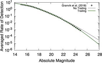
Figure 4. The CSS’s mean rate of detection—the number of CSS FOVs in which an NEO with given orbital elements is expected to be detected—is plotted as a function of the absolute magnitude (green line). The average of  , given in Equation (4), was computed over the whole orbital domain. The original bias from Granvik et al. (2018) is shown by open circles. The gray line shows the detection rate when the trailing loss from Zavodny et al. (2008) is not accounted for.
Download figure:
Standard image High-resolution imageThe detection probability of CSS is ≳0.7 for large, H ≃ 15 NEOs, except for those on orbits with a < 0.8 au (Figure 5). Fainter NEOs are detected with lower probability. Figure 6 illustrates these trends in more detail. Interestingly,  shows dips and bumps as a function of NEO’s semimajor axis (vertical strips in the top panels of Figure 5). The dips, where the detection probability is lower, correspond to the orbital periods that are integer multiplies of 1 yr. This is where the synodic motion of NEOs allow them to hide and not appear in the survey’s FOVs. This effect has been reported before (e.g., Tricarico 2017). The average detection rate is less sensitive to this effect because the hidden NEOs represent a relatively small fraction of the total sample and have a small weight in the average when the detection rate is considered.
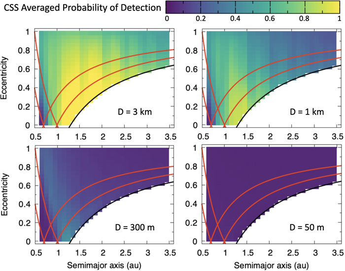
Figure 5. The CSS detection probability (Equation (5)) as a function of orbital elements for four different absolute magnitude values. From top left to bottom right, we plot  for H corresponding to objects with D = 3 km, 1 km, 300 m, and 50 m (H = 15.37, 17.75, 20.37, and 24.26 for the reference albedo pV = 0.14). The detection probability was averaged over all inclinations bins. The vertical strips, with
  going up and down as a function of the NEO’s semimajor axis, are discussed in the main text.
Download figure:
Standard image High-resolution image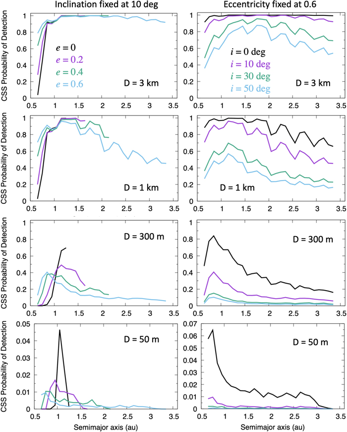
Figure 6. The CSS detection probability (Equation (5)) as a function of orbital elements for four different absolute magnitude values. From top to bottom, we plot  for H corresponding to objects with D = 3 km, 1 km, 300 m, and 50 m (H = 15.37, 17.75, 20.37, and 24.26 for the reference albedo pV = 0.14). The plots in the left column show
  for the fixed orbital inclination (i = 10°) and several eccentricity values. The plots on the right show
  for e = 0.6 and several inclination values. The detection probability was computed for orbits with q < 1.3 au.
Download figure:
Standard image High-resolution image5. Parameter Optimization with MultiNest
We use MultiNest to perform the model selection, parameter estimation, and error analysis (Feroz & Hobson 2008; Feroz et al. 2009). 26 MultiNest is a multimodal nested sampling routine (Skilling 2004) designed to compute the Bayesian evidence in a complex parameter space in an efficient manner. The parameter space may contain multiple posterior modes and degeneracies in high dimensions. For brevity, we direct those interested to the aforementioned works for further details.
We use the following reasoning to define the log-likelihood in MultiNest. Let nj be the number of objects detected by CSS in the bin j, and λj be the number of objects in the bin j expected from the model. Here the index j goes over all bins in a, e, i, and H. Assuming the Poisson distribution 27 with the expected number of events λj , the probability of drawing nj objects is

The joint probability over all bins is then
The log-likelihood can therefore be defined as

where we dropped the constant term  . This definition is identical to that used in Granvik et al. (2018), except that the present work uses the detection probability (not efficiency) and first detection (i.e., no multiple redetections; Section 4.1). The second term in Equation (8) is evaluated over all bins with detected objects. The first term penalizes models with large overall values of λj
. For two or more surveys,
. This definition is identical to that used in Granvik et al. (2018), except that the present work uses the detection probability (not efficiency) and first detection (i.e., no multiple redetections; Section 4.1). The second term in Equation (8) is evaluated over all bins with detected objects. The first term penalizes models with large overall values of λj
. For two or more surveys,  is simply the sum of individual survey’s log-likelihoods.
The models explored here range from simple ones with as few as seven parameters (three source weights and four magnitude distribution coefficients) to complex ones with as many as 30 parameters (12 sources with size-dependent contributions, cubic spline representation of the magnitude distribution, and magnitude-dependent disruption for bodies with low perihelion distance; Granvik et al. 2016). We first describe various issues that are common to these models and emphasize differences with respect to the previous work—the tested models are discussed in Sections 6 and 8.
The model selection is based on the evidence term  computed by MultiNest. The aim is to select one model from a set of competing models that represents most closely the underlying process that generated the observed data. The models are considered to be a priori equiprobable. To compare two models, we compute the ratio of their posterior probabilities (the Bayes factor;
  ) and use it to evaluate the statistical preference for the best one. Note that this procedure implicitly penalizes models with more parameters.
There are three sets of priors: (1) coefficients α that determine the strength of different sources, (2) parameters related to the absolute magnitude distribution, and (3) priors that define the disruption model. The motivation for (3) is explained in Section 5.3 (see Granvik et al. 2016). We limit our analysis to considerations based on the absolute magnitude distribution. The albedo and size distribution constraints from the Wide-field Infrared Survey Explorer (Mainzer et al. 2019) will be addressed in a forthcoming publication.
5.1. Strength of Sources
As for (1), the intrinsic orbital distribution of model NEOs is obtained by combining ns sources:  with
with  . The coefficients αj
represent the relative contribution of each source to the NEO population (i.e., the fraction of NEOs from the source j). The binned distribution p(a, e, i) is normalized to one NEO and needs to be supplemented by the absolute magnitude distribution (Section 5.2).
. The coefficients αj
represent the relative contribution of each source to the NEO population (i.e., the fraction of NEOs from the source j). The binned distribution p(a, e, i) is normalized to one NEO and needs to be supplemented by the absolute magnitude distribution (Section 5.2).
The main difficulty with implementing the α coefficients in MultiNest is that the Bayesian tools typically work with independent priors. It is therefore not possible, for example, to choose each αj randomly between 0 and 1, and rescale them later such that they sum to 1. Using a geometrical approach, we found the following general algorithm for assuring that αj have a multivariate, uniformly random distribution, and automatically sum to 1. We generate uniformly random deviates 0 ≤ Xj ≤ 1 and compute
for 1 ≤ j ≤ ns − 1, and
The order in which different sources are linked to the index j has no effect on the results. Kipping (2013) derived an identical formula for ns = 3. The problem in question is related to the Dirichlet distribution with equal weights, but it is not immediately obvious to us how to construct an efficient algorithm based on that (as the inverse cumulative distribution, CDF, is needed in Equation (9)).
The contribution of different sources to NEOs may be size dependent. This is because the weak orbital resonances in the inner belt are expected to produce an important share of large NEOs (Migliorini et al. 1998). Small main-belt asteroids instead drift across large radial distances by the Yarkovsky thermal effect (Vokrouhlický et al. 2015), can pass over the weak resonances, and reach the strong ν6 source (Granvik et al. 2017). Granvik et al. (2018) accounted for the size dependency by adopting a separate size distribution for each source (see Section 5.2). Here we set αj
coefficients to be functions of the absolute magnitude. For simplicity, we adopt a linear relationship,  , where Hα
is some reference magnitude, and
, where Hα
is some reference magnitude, and  and
and  are new model parameters. In practice, using Equations (9) and (10), we set
  and
and  for some minimum and maximum absolute magnitudes (e.g.,
  and
and  ), and linearly interpolate between them. This automatically assures that ∑j
αj
(H) = 1 for any
), and linearly interpolate between them. This automatically assures that ∑j
αj
(H) = 1 for any  .
.
5.2. Absolute Magnitude Distribution
The differential absolute magnitude distribution is denoted by  . Given that the magnitude distribution is not seen to wildly vary across the main belt (Heinze et al. 2019), and craters on the main-belt asteroids follow a common size distribution (Bottke et al. 2020), we use a similar setup for different main-belt sources. Specifically, the magnitude distribution produced by source j is set to be
  . The magnitude distributions of different sources are similar, but change with αj
(H), which are assumed to linearly vary with H (Section 5.1). For example, as the ν6 source is found to contribute more to faint NEOs than to bright NEOs (Section 6), the magnitude distribution of ν6 is slightly steeper than
. The magnitude distributions of different sources are similar, but change with αj
(H), which are assumed to linearly vary with H (Section 5.1). For example, as the ν6 source is found to contribute more to faint NEOs than to bright NEOs (Section 6), the magnitude distribution of ν6 is slightly steeper than  . When the contribution of different sources is combined, we find that ∑αj
(H)n(H)dH = n(H)dH, which means that n(H) stands for the absolute magnitude distribution of the whole NEO population. This is a convenient scheme.
. When the contribution of different sources is combined, we find that ∑αj
(H)n(H)dH = n(H)dH, which means that n(H) stands for the absolute magnitude distribution of the whole NEO population. This is a convenient scheme.
Our choice of  greatly limits the number of model parameters. For the cubic spline representation of
  (see below), and ns sources, we have 2ns + 5 parameters in total (2ns
α's and five parameters defining
(see below), and ns sources, we have 2ns + 5 parameters in total (2ns
α's and five parameters defining  ). For comparison, Granvik et al. (2018) used different magnitude distributions for individual sources, in which each distribution was represented by a third-order polynomial with four coefficients. This gives 4ns parameters in total. The setup in Granvik et al. (2018) can account for large magnitude-distribution differences between different sources. With too many parameters, however, the model can be over-parameterized, and not all of the parameters can be constrained from the existing observations.
Granvik et al. (2018) defined the magnitude distribution of each source using a smooth, second-degree variation of the differential slope. In terms of the log-cumulative magnitude distribution,  , this is equivalent to a third-order polynomial representation:
  , where Nref is the normalization constant, Href is some constant reference magnitude (Href = 17 in Granvik et al. 2018), γ is the slope of the linear term, and the cubic term is centered at Hc and has the “twist” amplitude δ. In this case, there are four free parameters for each source: Nref, γ, δ, and Hc.
We tested this parameterization in our model and found that it has undesired limitations. First,  , as given above, is symmetric around Hc, but the real magnitude distribution of NEOs is not symmetric; it is gently rounded just below H = 20 but has a sharper dip leading to a steeper slope for H > 20 (e.g., Harris & D’Abramo 2015). It then becomes difficult to accurately fit observations in this model because the cubic polynomial representation is simply too rigid. In Granvik et al. (2018), the asymmetric magnitude distribution of NEOs was composed from many different sources each having a symmetric distribution (around a different Hc value). This should have produced some tension in the fit. Second, given the rigid nature of the cubic polynomial with a twist, the fit near H = 25, where the magnitude distribution is steep, would influence the fit at H = 15. This is not desirable as the model should have enough flexibility to deal with the bright and faint bodies separately. Third, the cubic polynomial is difficult to generalize to a wider absolute magnitude range and/or higher accuracy. Higher-order polynomials, for example, have the inconvenient property that the polynomial coefficients sensitively depend on the order; they wildly change if the order is increased.
Here we use cubic splines to represent  . The magnitude interval of interest, 15 < H < 25 for our base CSS model (Section 6), is divided into several segments. The more sections there are, the more accurate the parameterization is, but we also have more parameters to deal with. After experimenting with different choices, we opted for four segments and five parameters. There are four parameters defining the average slope in each segment, γj
, and one parameter that provides the overall calibration. We typically use Nref = N(Href) with Href = 17.75 (diameter D = 1 km for the reference albedo pV = 0.14). The normalization constant and slope parameters are used to compute
. The magnitude interval of interest, 15 < H < 25 for our base CSS model (Section 6), is divided into several segments. The more sections there are, the more accurate the parameterization is, but we also have more parameters to deal with. After experimenting with different choices, we opted for four segments and five parameters. There are four parameters defining the average slope in each segment, γj
, and one parameter that provides the overall calibration. We typically use Nref = N(Href) with Href = 17.75 (diameter D = 1 km for the reference albedo pV = 0.14). The normalization constant and slope parameters are used to compute  at the boundaries between segments; cubic splines are constructed from that result (Press et al. 1992). The splines assure that N(H) smoothly varies with H. This representation has the desired properties: it is accurate, flexible, and can easily be generalized by adding more segments.
28
at the boundaries between segments; cubic splines are constructed from that result (Press et al. 1992). The splines assure that N(H) smoothly varies with H. This representation has the desired properties: it is accurate, flexible, and can easily be generalized by adding more segments.
28
Optionally, we can use additional constraints to inform the MultiNest fits. For example, the known sample of NEOs with H < 15 is complete, and there are ≃50 such objects in the JPL Small Bodies Database. 29 We can therefore fix N(15) = 50 and compute the γ1 slope such that this additional constraint is satisfied. With this, we only have four absolute magnitude distribution parameters in the MultiNest fit.
5.3. Disruption Model
To account for the disruption of NEOs at small perihelion distances, following Granvik et al. (2016), we eliminate test bodies when they reach critical distance q*. Granvik et al. (2016) found that q* is a function of size with small NEOs disrupting at larger perihelion distances than the large ones. To demonstrate this, Granvik et al. (2016) divided the absolute magnitude range into three intervals, H = 17–19, 20–22, and 23–25, and performed separate fits to CSS in these three cases. They found that q*(H) is roughly linear in H with q* ≃ 0.06 au for H = 17–19, q* ≃ 0.12 au for H = 20–22, and q* ≃ 0.18 au for H = 23–25. We tested the same method here and found results consistent with Granvik et al. (2016).
Performing separate fits in different magnitude ranges is somewhat awkward (because there are many other parameters to explore as well). Granvik et al. (2018) therefore used a different method where the effect of disruptions was approximated by a penalty function P(a, e) = 1 − k[q0 − a(1 − e)] for q < q0 and P(a, e) = 1 otherwise. The two parameters of the penalty function, k and q0, which have some (unspecified) relationship to q*, were estimated from the CSS fit (Granvik et al. 2018). Given that the penalty function only depends on a and e, this method cannot accurately reproduce the real effect of disruptions. This is because, when bodies are removed at q*, this not only affects the (a, e) distribution but also influences the inclination distribution (it becomes narrower for shorter lifetimes) and absolute magnitude distribution (as q* is size dependent). We find that this is not a minor issue (Figure 7).
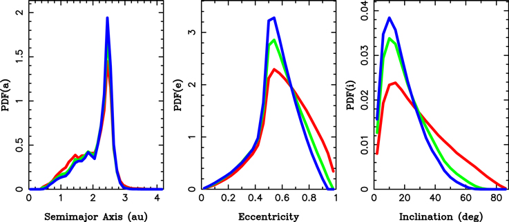
Figure 7. The orbital distributions of NEOs from the 3:1 source for three disruption thresholds: q* = 0.005 au (red line), q* = 0.1 au (green line), and q* = 0.2 au (blue line). By increasing the disruption distance in the model, we remove the orbits with high eccentricities, and the eccentricity distribution becomes more peaked near e = 0.5. At the same time, the inclination distribution becomes narrower.
Download figure:
Standard image High-resolution imageTo circumvent these problems, here we assume that the q* dependence on H is roughly linear, and parameterize it by q* = q0* + δ q*(H − Hq ), where Hq = 20. We use uniform priors for the two parameters, q0* and δ q*. To construct the orbital distribution for any q* < 0.3 au, we first produce the binned distributions (from each source) for q* = 0, 0.05, 0.1, 0.15, 0.2, 0.25, and 0.3 au. This is done by following the orbit of every simulated object and recording the time t* when the object reached q < q* for the first time. The binning is done for t < t*. The object is assumed to disrupt at t = t* and is not included for t > t*. The fitting routine then linearly interpolates between distributions obtained with different q* to any intermediate value of q*(H). The resulting orbital distribution, pq*, which now also depends on the absolute magnitude, pq* = pq*(a, e, i, H), is normalized to 1 (∫pq*(a, e, i, H) da de di = 1 for any H).
The method described above assures that a single fit can be performed globally, for the full range of H, and at the same time we are using a physically based approach to modeling the size/magnitude-dependent disruption distance. The linear dependence of q* on H could be generalized to a more complex functional form when the need for that arises.
5.4. Model Summary
In summary, our biased NEO model is
where αj
are the magnitude-dependent weights of different sources (∑j
αj
(H) = 1), ns
is the number of sources, pq*,j
(a, e, i, H) is the PDF of the orbital distribution of NEOs from the source j, including the size-dependent disruption at the perihelion distance q*(H) (this is the only H-dependence in the p functions), n(H) is the differential absolute magnitude distribution of the NEO population (the log-cumulative distribution is given by splines; Section 5.2), and  is the CSS detection probability (Equation (5)). For each MultiNest trial, Equation (11) is constructed by the methods described above. This defines the expected number of events
  in every bin of the model domain, and allows MultiNest to evaluate the log-likelihood from Equation (8).
The intrinsic (debiased) NEO model is simply
By integrating Equation (12) over the orbital domain, given that ∫pq*,j (a, e, i, H) da de di = 1 and ∑j αj (H) = 1, we verify that n(H) stands for the (differential) magnitude distribution of the whole NEO population.
6. The Base NEO Model
Our base NEO model accounts for ns = 12 sources. Each source has a magnitude-dependent contribution (Section 5.1) and the source weights αj (15) (for H = 15) and αj (25) (for H = 25) therefore represent 2(ns − 1) model parameters (the last source’s contribution is computed from Equation (10)). There are four parameters related to the magnitude distribution, Nref and γj , 2 ≤ j ≤ 4 (15 ≤ H ≤ 25). The γ1 parameter is fixed such that N(15) = 50 (Section 5.2). In addition, the q0* and δ q* parameters define the disruption model. This adds to 28 model parameters in total. We used uniform priors for all parameters (see Section 5.1 for the multivariate uniform distribution of αj (15) and αj (25)). The CSS fits were executed with the MultiNest code running on 2000 Ivy Bridge cores of the NASA Pleiades Supercomputer. Each fit required at least four wall-clock hours to fully converge.
The base model, as presented here, was identified by the Bayes factor analysis (Section 5). We generated a large number of rival models (about 50; Section 8) and computed their Bayes factors relative to the base model. These models tested the magnitude-independent αj
, disregarded disruption of NEOs at small perihelion distances, adopted constant q* (independent of H), etc. The analysis showed an overwhelming statistical preference for the base model,  . For example, the nondisruption and constant-α models are disfavored by
  relative to
  . The models with fewer than 12 sources are disfavored by at least 5σ relative
  , except for the models without 7:3, 9:4, JFCs, or 11:5 (see below). There is a correlation between
  and ns with higher-ns models generally giving higher Bayesian evidences. This probably means that the NEO population is supplied from a large number of sources and the CSS observations are sufficiently diagnostic to establish that.
Four rival models showed evidence terms comparable to the base model. The 11-source models without the 7:3, 8:3, or JFC sources are favored by factors of 33, 18, and 3.7, respectively, relative to the base model. The model without the 11:5 source is disfavored by a factor of 8.2 relative to the base model. This means that the optimal model would be a nine-source model without 7:3, JFCs, and 9:5 (but keeping 11:5). Here we prefer to report the results of the 12-source base model, because some of the Bayes factors reported above are relatively small. The base model also provides upper limits on the contribution of these weak sources (see below).
MultiNest provides the posterior distribution of model parameters (Figure 8). 30 The posterior distribution is well behaved for most parameters (i.e., unimodal and Gaussian-like). In some cases, the fit provides an upper bound on the contribution of a specific source. This most clearly happens for the 7:3 and 9:4 resonances, which are located in the sparsely populated region of the outer belt, and for JFCs. We use the posterior distribution to compute the median and standard 1σ (68.3% confidence interval) uncertainties of model parameters (Table 3). For parameters, for which the posterior distribution peaks near zero (e.g., the contribution of 7:3, 9:4, and JFCs), we also report the upper limit in Table 3. For bright NEOs, for which the contribution of these weak sources was found to be slightly more substantial, we obtained α7:3(15) < 0.012, α9:4(15) < 0.020, and αJFC(15) < 0.017 (68.3% envelopes). The contribution of JFCs to the NEO population is inferred to be smaller than in previous works (e.g., ≃6% contribution in Bottke et al. 2002; and 2%–10% H-dependent contribution in Granvik et al. 2018). For faint NEOs (H ≃ 25), all middle and outer belt resonances, except for 5:2, have α(25) < 0.02 (68.3% envelopes). This implies that the contribution of the middle/outer belt to very small NEOs is minor.
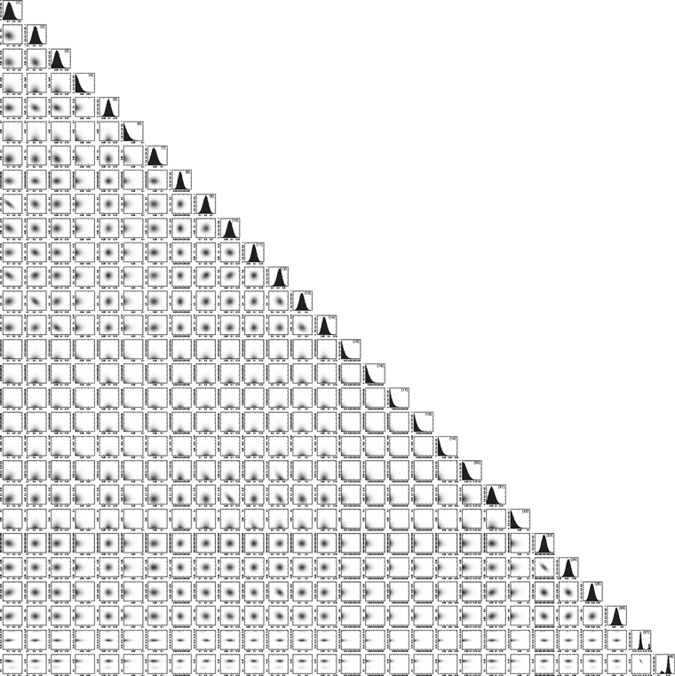
Figure 8. The posterior distribution of 28 NEOMOD parameters from our base MultiNest fit to CSS. The individual plots are labeled (1) to (28) following the model parameter sequence given in Table 3.
Download figure:
Standard image High-resolution imageTable 3. Median and Uncertainties of Our Base Model Parameters
| Label | Parameter | Median | −σ | +σ | Limit |
|---|---|---|---|---|---|
| α's for H = 15 | |||||
| (1) | ν6 | 0.118 | 0.052 | 0.056 | ⋯ |
| (2) | 3:1 | 0.219 | 0.040 | 0.041 | ⋯ |
| (3) | 5:2 | 0.057 | 0.026 | 0.028 | ⋯ |
| (4) | 7:3 | 0.008 | 0.005 | 0.009 | 0.012 |
| (5) | 8:3 | 0.093 | 0.020 | 0.021 | ⋯ |
| (6) | 9:4 | 0.013 | 0.009 | 0.017 | 0.020 |
| (7) | 11:5 | 0.044 | 0.020 | 0.022 | ⋯ |
| (8) | 2:1 | 0.045 | 0.010 | 0.010 | ⋯ |
| (9) | inner weak | 0.202 | 0.048 | 0.045 | ⋯ |
| (10) | Hungarias | 0.082 | 0.022 | 0.022 | ⋯ |
| (11) | Phocaeas | 0.095 | 0.017 | 0.018 | ⋯ |
| ⋯ | JFCs | 0.012 | 0.008 | 0.013 | 0.017 |
| α's for H = 25 | |||||
| (12) | ν6 | 0.424 | 0.043 | 0.040 | ⋯ |
| (13) | 3:1 | 0.338 | 0.034 | 0.035 | ⋯ |
| (14) | 5:2 | 0.063 | 0.018 | 0.020 | ⋯ |
| (15) | 7:3 | 0.004 | 0.003 | 0.006 | 0.007 |
| (16) | 8:3 | 0.010 | 0.008 | 0.014 | 0.016 |
| (17) | 9:4 | 0.007 | 0.005 | 0.010 | 0.012 |
| (18) | 11:5 | 0.009 | 0.007 | 0.013 | 0.014 |
| (19) | 2:1 | 0.006 | 0.004 | 0.008 | 0.009 |
| (20) | inner weak | 0.033 | 0.023 | 0.036 | 0.049 |
| (21) | Hungarias | 0.056 | 0.027 | 0.030 | ⋯ |
| (22) | Phocaeas | 0.014 | 0.010 | 0.018 | 0.021 |
| ⋯ | JFCs | 0.008 | 0.006 | 0.011 | 0.014 |
| H distribution | |||||
| (23) | Nref | 896 | 29 | 29 | ⋯ |
| (24) | γ2 | 0.344 | 0.006 | 0.006 | ⋯ |
| (25) | γ3 | 0.328 | 0.004 | 0.004 | ⋯ |
| (26) | γ4 | 0.566 | 0.014 | 0.014 | ⋯ |
| Disruption parameters | |||||
| (27) |

| 0.144 | 0.004 | 0.007 | ⋯ |
| (28) | δ q* | 0.030 | 0.003 | 0.001 | ⋯ |
Note. The first column is the parameter/plot label in Figure 8 (JFCs do not appear in the figure). The uncertainties reported here were obtained from the posterior distribution produced by MultiNest. They do not account for uncertainties of the CSS detection efficiency. For parameters, for which the posterior distribution shown in Figure 8 peaks near zero, the last column reports the upper limit (68.3% of posteriors fall between zero and that limit).
Download table as: ASCIITypeset image
We note several correlations between model parameters. A notable degeneracy is related to the contribution of the ν6 resonance and weak resonances in the inner main belt (Figure 9). The orbital distributions produced by these sources are similar, and MultiNest has difficulty in distinguishing between them for H = 15. Bottke et al. (2002) already discussed a related degeneracy between the ν6 resonance and their intermediate Mars crossers source. There is a hint of correlation between ν6 and weak resonances even for H = 25, where we only have an upper limit on the contribution of inner resonances. Faint NEAs detected by CSS are apparently more diagnostic for distinguishing these two sources. 31
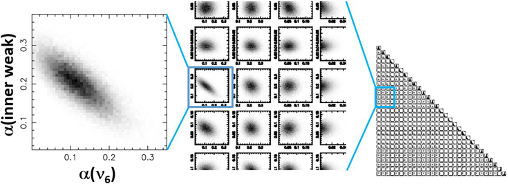
Figure 9. The enlarged plot on the left illustrates the degeneracy between contributions of the ν6 resonance and weak resonances in the inner belt to bright NEOs (H = 15). The two contributions are anticorrelated and sum up to ≃30%.
Download figure:
Standard image High-resolution imageAdditional correlations can be identified in Figure 8. For example, Nref and γ2 are anticorrelated (labels 23 and 24 in Figure 8), indicating that the models with lower Nref require a steeper magnitude slope for 17.5 < H < 20. Interestingly, the contributions of some individual sources, such as ν6, 3:1 and 5:2, to faint and bright NEOs are anticorrelated. We speculate that this happens because the total contribution of a source to faint and bright NEOs is relatively well constrained from CSS. A smaller contribution for H = 15 would then require a larger contribution for H = 25 for things to balance. Other possibilities exist as well.
The biased base model  is compared to CSS NEO detections in Figures 10 and 11. The distributions in Figure 10 are broadly similar. The 1D PDFs in Figure 11 show the comparison in more detail. The model distribution in Figure 11(a) has the overall shape of CSS observations, but the two semimajor-axis peaks at 1.5–2.4 au do not exactly align (they are shifted by 0.1–0.2 au). Statistical fluctuations may be responsible for this difference. We applied the Kolmogorov–Smirnov (K-S) test to CDFs corresponding to the distributions shown in Figure 11 and found that the semimajor axis model distribution is not rejectable (K-S probability 9.7%). The model e, i, and H distributions match observations well (K-S probabilities of 14%, 32%, and 61% for the eccentricity, inclination, and absolute magnitude, respectively).
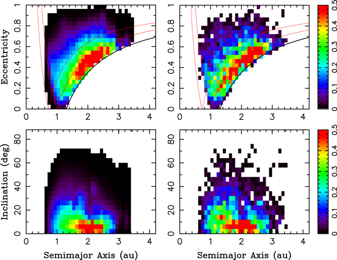
Figure 10. The orbital distribution of NEOs from our biased based model (left panels) and the CSS NEO detections (right panels). The two distributions were binned with the same resolution and are shown here in the (a, e) and (a, i) projections. There are no NEOs with the aphelion inside Venus orbit in CSS (and the biased model), because the pointing strategy of CSS had negligible low solar-elongation coverage.
Download figure:
Standard image High-resolution image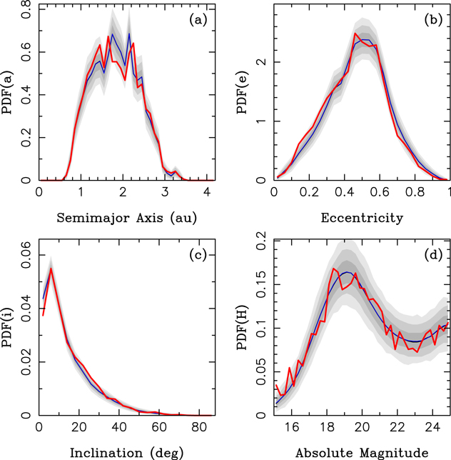
Figure 11. The probability density functions (PDFs) of a, e, i, and H from our biased base best-fit model (blue lines) and the CSS NEO detections (red lines). The shaded areas are 1σ (bold gray), 2σ (medium), and 3σ (light gray) envelopes. We used the best-fit solution (i.e., the one with the maximum likelihood) from the base model and generated 30,000 random samples with 3803 NEOs each (the sample size identical to the number of CSS’s NEOs in the model domain; 15 < H < 25). The samples were biased and binned with the standard binning (Table 2). We identified envelopes containing 68.3% (1σ), 95.5% (2σ), and 99.7% (3σ) of samples and plotted them here. The K-S test probabilities are 9.7%, 14%, 32%, and 61% for the a, e, i, and H distributions, respectively.
Download figure:
Standard image High-resolution imageThe base model correctly reproduces various orbital correlations with H. To demonstrate this, we slice PDFs using different absolute magnitude ranges and show the results in Figure 12. For example, the inclination distribution for H = 15–20 is broader than the one for H = 20–25. The eccentricity distribution is pyramidal in shape for H = 15–20 and becomes more peaked for H = 20–25. An interesting feature, which is not reproduced quite well in the model, is the population of faint NEOs with H = 20–25, a ≃ 1–1.6 au and e < 0.4 (K-S test probabilities 10−4 and 0.012 for a and e, respectively). This population is not present in the CSS detections for H < 20 and gradually appears for fainter NEOs.
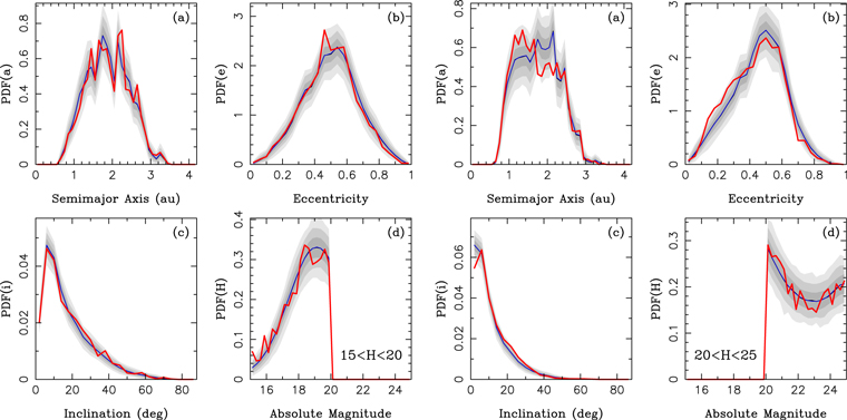
Figure 12. The PDFs of a, e, i, and H from our biased base best-fit model (blue lines) are compared to the CSS NEO detections (red lines). The four panels on the left show the results for bright NEOs with 15 < H < 20, and the four panels on the right show the results for faint NEOs with 20 < H < 25. The shaded areas are 1σ (bold gray), 2σ (medium), and 3σ (light gray) envelopes. See caption of Figure 11 for the method that we used to compute these envelopes. For 20 < H < 25, the K-S test probabilities are 10−4 and 0.012 for the a and e distributions, respectively.
Download figure:
Standard image High-resolution imageThe intrinsic (debiased) absolute magnitude distribution from our base model is shown in Figure 13. It is practically identical (<2 σ difference for 17 < H < 25) to that reported in Harris & Chodas (2021). For H < 17, the 3σ envelope shown in Figure 12 shrinks because we fixed N(15) = 50—here the NEO population given in Harris & Chodas (2021) is slightly higher. For reference, Harris & Chodas (2021) obtained 4,625, 15,880, and 3.13 × 10⁵ NEOs with H < 19.75, H < 21.75, and H < 24.75, respectively (the magnitude cuts are given here to avoid problems with rounding of the magnitude values reported by JPL/MPC; Harris & Chodas 2021). No error estimates were reported in Harris & Chodas (2021). From our base model, we find 4580 ± 160, 16020 ± 550, and (2.89 ± 0.15) × 105 NEOs with H < 19.75, H < 21.75, and H < 24.75, respectively, in very close agreement with Harris & Chodas (2021). The relative 1σ uncertainty of our estimates gradually increases from ≃3% for H < 20 to ≃6% for H < 25. The uncertainty reported here was computed from the MultiNest posterior sample and does not account for various uncertainties related to the CSS detection efficiency (Sections 4.3 and 4.4). As the CSS detection efficiency uncertainty likely increases with H (e.g., due to issues related to the trailing loss; Section 4.4), our NEO-population estimates should become significantly more uncertain for faint magnitudes (H ≳ 25). 32 The magnitude distribution in the extended magnitude range 15 < H < 28 is discussed in Sections 8 and 10.
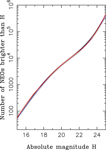
Figure 13. The intrinsic (debiased) absolute magnitude distribution of NEOs from our base model (the black line is the median and the blue line is the best fit) is compared to the magnitude distribution from Harris & Chodas (2021; red line). The gray area is the 3σ envelope obtained from the posterior distribution computed by MultiNest. It contains—by definition—99.7% of our base model posteriors.
Download figure:
Standard image High-resolution imageHeinze et al. (2019) estimated the slope of the absolute magnitude distribution for main-belt asteroids. They found γ ≃ 0.22 for H = 20–23.5 and γ ≃ 0.34 for H = 23.5–25.6. Here our base NEO-population model suggests γ ≃ 0.328 ± 0.004 for H ≃ 20 (Table 3) and a steeper slope for H ≃ 25 (γ ≃ 0.566 ± 0.014). This is roughly consistent with the results of Heinze et al. (2021), who found γ = 0.31–0.34 for NEOs with H ≃ 18–22 and γ = 0.54–0.57 for NEOs with H ≃ 23–28. The magnitude distribution of NEOs for 20 ≲H ≲25 therefore appears to be significantly steeper (>5 σ difference) than that of main-belt asteroids, but not much steeper (≃0.1–0.2 difference in the slope index γ). This result is most likely related to the size-dependent delivery of main-belt asteroids, via the Yarkovsky thermal force, to source resonances (e.g., Morbidelli & Vokrouhlický 2003).
Various issues related to the photometric detection efficiency of CSS limit our ability to accurately predict the number of kilometer-sized NEOs. The MultiNest fit gives N(17.75) = 931 ± 30 (H = 17.75 corresponds to D = 1 km for pV = 0.14), but the uncertainty given here does not account for the uncertainty in the CSS detection efficiency.
33
As we noted in Section 4, the uncertainties of parameters 0,
 , and Vwidth were not given in Jedicke et al. (2016). Ideally, we would need these uncertainties on a nightly basis. The changes of
 0 from night to night of CSS observations, which could be taken as a very conservative proxy for the uncertainty in the detection probability of bright NEOs, are ∼10% (Jedicke et al. 2016). The accurate characterization of survey’s detection efficiency and its uncertainty is of the foremost importance for accurate population estimates.
We find that different main-belt sources have different contributions to small and large NEOs (Figure 14). The models with the size-independent contribution of different sources are statistically disfavored ( relative to the base model) and can be ruled out. This relates back to Valsecchi & Gronchi (2015), who pointed out that the orbital distribution of bright NEOs (H < 16) is significantly different from the model distribution in Bottke et al. (2002). Granvik et al. (2018) already identified some complex size dependence in the NEO delivery process. Other works also speculated that the delivery process is size dependent (e.g., Nesvorný et al. 2021). Here we find that the ν6 and 3:1 resonances jointly contribute to ≃30% of H = 15 NEOs and ≃80% of H = 25 NEOs.
34
This most likely happens because small main-belt asteroids radially drift by the Yarkovsky effect, pass through weak resonances, and reach the powerful ν6 and 3:1 resonances. Large main-belt asteroids do not move much and are more likely to be removed from the asteroid belt by weaker resonances (Migliorini et al. 1998; see also Section 10.1). The ν6 resonance shows the strongest dependence on size with the ≃10% contribution for H = 15 and ≃40% contribution for H = 25. The weak resonances in the inner main belt are found to produce over 20% of NEOs with H = 15, but their share drops to <7% (1σ limit) for H = 25 (Table 3). The contributions of ν6 and inner main-belt resonances show an anticorrelated dependence on size (Figure 14).
relative to the base model) and can be ruled out. This relates back to Valsecchi & Gronchi (2015), who pointed out that the orbital distribution of bright NEOs (H < 16) is significantly different from the model distribution in Bottke et al. (2002). Granvik et al. (2018) already identified some complex size dependence in the NEO delivery process. Other works also speculated that the delivery process is size dependent (e.g., Nesvorný et al. 2021). Here we find that the ν6 and 3:1 resonances jointly contribute to ≃30% of H = 15 NEOs and ≃80% of H = 25 NEOs.
34
This most likely happens because small main-belt asteroids radially drift by the Yarkovsky effect, pass through weak resonances, and reach the powerful ν6 and 3:1 resonances. Large main-belt asteroids do not move much and are more likely to be removed from the asteroid belt by weaker resonances (Migliorini et al. 1998; see also Section 10.1). The ν6 resonance shows the strongest dependence on size with the ≃10% contribution for H = 15 and ≃40% contribution for H = 25. The weak resonances in the inner main belt are found to produce over 20% of NEOs with H = 15, but their share drops to <7% (1σ limit) for H = 25 (Table 3). The contributions of ν6 and inner main-belt resonances show an anticorrelated dependence on size (Figure 14).
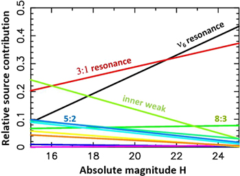
Figure 14. The contribution of different NEO sources as a function of the absolute magnitude. The ν6 and 3:1 resonances are shown by the black and red lines, respectively. The light-green line is the contribution of weak resonances in the inner main belt. The plot shows the result for the maximum likelihood parameter set from the base model. We simply plot αj (15) and αj (25) for each source and connect them by a straight line (Section 5.1). The uncertainties of αj (15) and αj (25) are listed in Table 3.
Download figure:
Standard image High-resolution imageWe confirm the need for the size-dependent disruption of NEOs at small perihelion distances as originally pointed out in Granvik et al. (2016). The models without disruption are statistically disfavored ( relative to the base model) and can be ruled out. Clearly, any model where the disruption is not taken into account produces a strong excess of low-q (or high-e) orbits. The q*(H) dependence found here roughly matches the one inferred in Granvik et al. (2016), which is perhaps not that surprising given that we use similar methodology and constraints as Granvik et al. (2016). Figure 15 shows the maximum likelihood base model with q*(18) ≃ 0.08 au (compared to q* ≃ 0.06 au for 17 < H < 19 in Granvik et al. 2016) and q*(24) ≃ 0.2 au (compared to q* ≃ 0.18 au for 23 < H < 25 in Granvik et al.). Based on this result, we could tentatively suggest that the NEO disruption happens at a slightly larger perihelion distance than found in Granvik et al. (2016). However, given that there is some variability between different models (Section 8), we believe that more work is needed to establish the q*(H) dependence with more confidence.
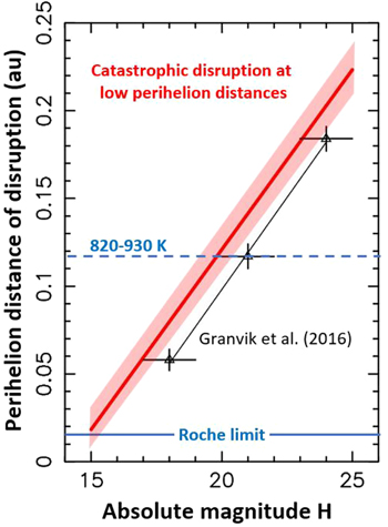
Figure 15. Disruption models. Our base model  , where the critical perihelion distance q* is assumed to be a linear function of absolute magnitude (the red line with the light-red envelope containing 68% of posteriors), is compared to Granvik et al. (2016; triangles with error bars). The surface temperature is estimated to be 820 K (average) and 930 K (subsolar) at 0.117 au (Granvik et al. 2016).
Download figure:
Standard image High-resolution imageThe size-dependent contribution of main-belt sources and the size-dependent disruption of NEOs at small perihelion distances imply that the orbital distribution of NEOs must be size-dependent as well. Figure 16 compares the orbital distributions of large (15 < H < 17.5) and small (22.5 < H < 25) NEOs. There are several differences. The eccentricity and inclination distributions of large NEOs are more extended than those of small NEOs. This is a direct consequence of the size-dependent disruption that favors removal of small NEOs with e > 0.6. The inclination distribution of large NEOs is more extended because large NEOs are less likely to be disrupted; they tend to survive longer, thus allowing the inclination distribution to become increasingly wider over time.
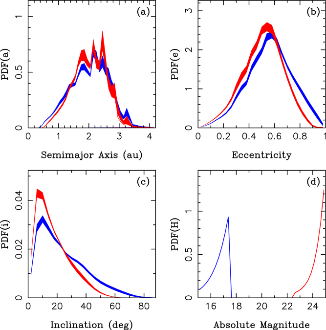
Figure 16. The PDFs of a, e, i, and H from the intrinsic (debiased) base model. The plot compares the distributions of bright NEOs with 15 < H < 17.5 (blue) and faint NEOs with 22.5 < H < 25 (red). The blue and red shaded areas are the 1σ envelopes of our base model posteriors.
Download figure:
Standard image High-resolution imageThe results presented here can be used to estimate the completeness of the currently known NEO population. We illustrate the current completeness for H < 22 in Figure 17. We find that the known population of H < 22 NEOs is roughly a factor of 2 incomplete (≃10,000 known versus 18,900 ± 700 estimated; Table 4). Undiscovered NEOs populate a wide range of orbits. The incompleteness rapidly increases toward fainter magnitudes. For example, for H < 25, our model predicts that there are ≃20 times more NEOs than currently known (i.e., the known population is only ≃5% complete). For H ≃ 25, we only know 1 in ≃100 NEOs (see the differential distribution in the bottom-right panel of Figure 17). We discuss the NEO population completeness in more detail in Sections 8 and 10.
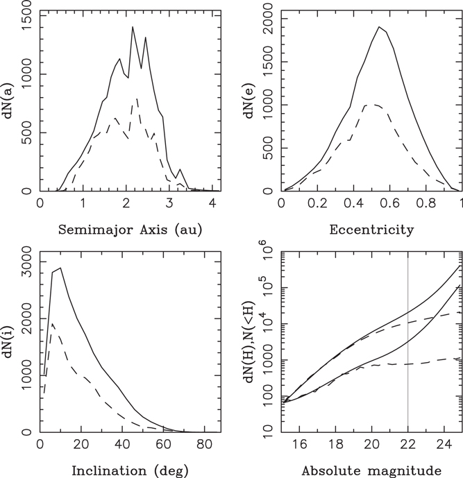
Figure 17. The incompleteness of the known NEO population. For the a, e, and i distributions, the dashed lines show the number of known NEOs with H < 22, and the solid lines are the number of NEOs with H < 22 inferred from our maximum likelihood base model (both given per bin interval; 0.1 au, 004, and 4°). For the H distribution in the bottom-right panel, we show both the cumulative and differential (per 0.25 mag) distributions (upper and lower lines, respectively; solid for model, dashed for known). The uncertainty of the cumulative population estimates increases from ≃3% for H < 20 to ≃6% for H < 25. The uncertainties were obtained from the posterior distribution produced by MultiNest and do not account for various uncertainties of the CSS detection efficiency.
Download figure:
Standard image High-resolution imageTable 4. Cumulative Number of NEOs
| H |

| H |

| H |

| H |

|
|---|---|---|---|---|---|---|---|
| 15.1 | 55.8 | 17.6 | 783.3 | 20.1 | 5795 | 22.6 | 28970 |
| 15.2 | 62.4 | 17.7 | 860.9 | 20.2 | 6180 | 22.7 | 31320 |
| 15.3 | 69.7 | 17.8 | 945.1 | 20.3 | 6585 | 22.8 | 33930 |
| 15.4 | 77.9 | 17.9 | 1036.3 | 20.4 | 7011 | 22.9 | 36850 |
| 15.5 | 87.0 | 18.0 | 1134.9 | 20.5 | 7458 | 23.0 | 40120 |
| 15.6 | 97.2 | 18.1 | 1241.4 | 20.6 | 7930 | 23.1 | 43780 |
| 15.7 | 108.6 | 18.2 | 1356.3 | 20.7 | 8427 | 23.2 | 47910 |
| 15.8 | 121.2 | 18.3 | 1480.1 | 20.8 | 8953 | 23.3 | 52580 |
| 15.9 | 135.2 | 18.4 | 1613.2 | 20.9 | 9509 | 23.4 | 57870 |
| 16.0 | 150.8 | 18.5 | 1756.1 | 21.0 | 10100 | 23.5 | 63880 |
| 16.1 | 168.1 | 18.6 | 1909.4 | 21.1 | 10730 | 23.6 | 70760 |
| 16.2 | 187.3 | 18.7 | 2073.6 | 21.2 | 11400 | 23.7 | 78630 |
| 16.3 | 208.5 | 18.8 | 2249.2 | 21.3 | 12110 | 23.8 | 87670 |
| 16.4 | 232.0 | 18.9 | 2436.8 | 21.4 | 12870 | 23.9 | 98100 |
| 16.5 | 258.0 | 19.0 | 2636.8 | 21.5 | 13690 | 24.0 | 110200 |
| 16.6 | 286.7 | 19.1 | 2849.7 | 21.6 | 14570 | 24.1 | 124200 |
| 16.7 | 318.4 | 19.2 | 3076.1 | 21.7 | 15520 | 24.2 | 140500 |
| 16.8 | 353.2 | 19.3 | 3316.5 | 21.8 | 16540 | 24.3 | 159500 |
| 16.9 | 391.6 | 19.4 | 3571.3 | 21.9 | 17650 | 24.4 | 181400 |
| 17.0 | 433.7 | 19.5 | 3841.0 | 22.0 | 18860 | 24.5 | 206900 |
| 17.1 | 479.9 | 19.6 | 4126.1 | 22.1 | 20180 | 24.6 | 236400 |
| 17.2 | 530.4 | 19.7 | 4426.9 | 22.2 | 21620 | 24.7 | 270500 |
| 17.3 | 585.7 | 19.8 | 4743.9 | 22.3 | 23200 | 24.8 | 309800 |
| 17.4 | 646.0 | 19.9 | 5077.3 | 22.4 | 24940 | 24.9 | 355200 |
| 17.5 | 711.8 | 20.0 | 5427.6 | 22.5 | 26850 | 25.0 | 407400 |
Note. For each absolute magnitude limit (H), the table reports the number of NEOs brighter than H as estimated from our base model ( ). The relative 1σ uncertainty of the population estimates given here increases from ≃3% for H < 20 to ≃6% for H < 28. The uncertainties were estimated from the posterior distribution produced by MultiNest. They do not account for uncertainties of the CSS detection efficiency.
Download table as: ASCIITypeset image
To aid similar estimates, and help to plan future observations, we developed the NEOMOD Simulator. The code inputs the base (or any other) model from MultiNest, provided as an ASCII table, and generates a user-defined sample of NEOs with the smooth orbital and absolute magnitude distributions. The NEOMOD Simulator will be available from GitHub. 35 Figure 18 illustrates an example output from the NEOMOD Simulator, where the user requested to generate the full sample of H < 25 NEOs from the base model described here. Statistically different NEO samples can be obtained by initializing the code with different random seeds.
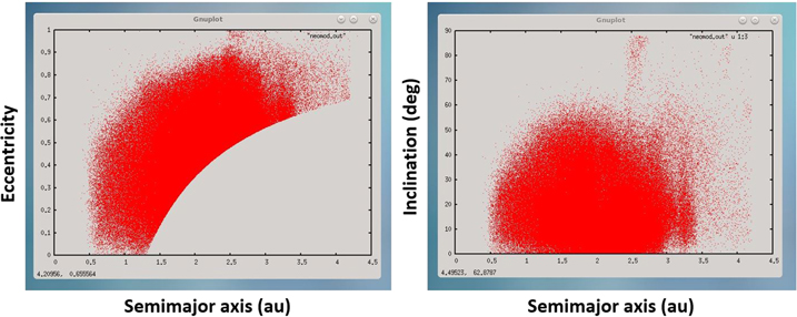
Figure 18. A sample output from the NEOMOD Simulator that shows ≃4.1 × 10⁵ orbits of NEOs with H < 25.
Download figure:
Standard image High-resolution imagePotentially hazardous objects (PHOs) are defined as having a minimum orbit intersection distance (MOID) with Earth of < 0.05 au (19.5 lunar distances) and H ≤ 22 (D ≃ 140 m for pV = 0.14). We used the code described in Wiźniowski & Rickman (2013) to estimate the number of PHOs as a function of orbital elements. Ten-thousand objects were placed into each orbital bin in a, e, and i, their nodal and perihelion longitudes were drawn from a uniformly random distribution, and MOID was computed for each orbit. We then evaluated the fraction of PHOs, following the definition above (MOID <0.05 au), in each bin. The PHO fraction is the largest for orbits with q ∼ 1 au, Q = a(1 + e) ∼ 1 au, a ∼ 1 au, and/or i < 10°. Figure 19 shows the completeness of the currently known PHO population. The trends seen here are similar to those discussed for the whole NEO population above. The bulk of yet-to-be-discovered PHOs have orbits with 1.2 < a < 2.8 au, moderate to large eccentricities, and i ≲ 40°. The PHO population completeness is >90% for a < 1.2 au, e < 0.3 and H < 22. This is because NEOs on these orbits have low MOID and can be more easily detected than NEOs in general. We find that there are 4000 ± 150 PHOs with H < 22 in total, of which ≃2300 are known. The overall population completeness is slightly higher for PHOs (≃58%) than for H < 22 NEOs in general (≃52%).
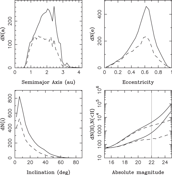
Figure 19. The incompleteness of the known PHO population (MOID <0.05 au, H < 22). For the a, e, and i distributions, the dashed lines show the number of known PHOs with H < 22, and the solid lines are the number of PHOs with H < 22 inferred from our maximum likelihood base model (both given per bin interval; 0.1 au, 004 and 4°). For the H distribution in the bottom-right panel, we show both the cumulative and differential (per 0.25 mag) distributions (upper and lower lines, respectively; solid for model, dashed for known). The uncertainty of the cumulative population estimates increases from ≃3% for H < 20 to ≃6% for H < 25. The uncertainties were obtained from the posterior distribution produced by MultiNest and do not account for various uncertainties of the CSS detection efficiency.
Download figure:
Standard image High-resolution image7. Planetary Impacts
Planetary impacts were recorded by the N-body integrator (Section 3). The record accounts for impacts of bodies with q < 1.3 au (NEOs) and q > 1.3 au (e.g., Mars crossers). We thus have complete information to determine the impact flux on all terrestrial planets, including Mars. We followed 105 test bodies from each source and have good statistics even from distant main-belt sources (e.g., 9:4 and 2:1). We find, in line with the results reported previously (e.g., Gladman et al. 1997; Bottke et al. 2006), that the impact probability per one body inserted in the source, pimp, strongly declines with the heliocentric distance of that source. For example, Hungarias, ν6 and weak inner-belt resonances have pimp ≃ 0.01–0.02 for impacts on the Earth, but pimp ≃ 10−4 for the outer-belt resonances such as 2:1 (Table 5). This happens for two reasons. First, the NEOs produced by distant sources typically end up having larger a and e, and thus lower (intrinsic) impact probabilities with the Earth. Second, these NEOs have shorter dynamical lifetimes, τ (defined as the time interval spent with q < 1.3 au) and are often removed before they can impact. For example, the ν6 source has τ ≃ 6.6 Myr for a reference value q* = 0.1 au, and impacts from ν6's NEOs on the Earth thus happen over this relatively long time interval. The 2:1 resonance produces much shorter lifetimes (e.g., τ ≃ 0.41 Myr for q* = 0.1 au).
Table 5. Average Lifetime of NEOs (τ), Earth-impact Probability (pimp), and Impact Flux (fimp = pimp/τ)
| Source | τ | pimp | fimp |
|---|---|---|---|
| (Myr) | (Myr−1) | ||
| ν6 | 6.64 | 0.02035 | 0.00306 |
| 3:1 | 1.38 | 0.00273 | 0.00198 |
| 5:2 | 0.29 | 0.00041 | 0.00141 |
| 7:3 | 0.15 | 0.00006 | 0.00041 |
| 8:3 | 1.20 | 0.00138 | 0.00149 |
| 9:4 | 0.21 | 0.00028 | 0.00132 |
| 11:5 | 0.29 | 0.00009 | 0.00029 |
| 2:1 | 0.41 | 0.00010 | 0.00025 |
| inner weak | 4.83 | 0.01262 | 0.00261 |
| Hungarias | 20.88 | 0.02802 | 0.00134 |
| Phocaeas | 15.33 | 0.00666 | 0.00043 |
Note. The values are given here for the fixed reference disruption distance q* = 0.1 au.
Download table as: ASCIITypeset image
Once the contribution of different sources to the NEO population is fixed,
36
via the weights αj
, we may ask how important each source is for planetary impacts. For that, we must fold in both pimp and τ. The best way to accomplish this is to consider the impact flux, fimp, which is related to the impact probability and lifetime by fimp = pimp/τ. Interestingly, the impact flux shows a much weaker dependence on the heliocentric distance of a source than the impact probability (Table 5). The low impact probabilities from more distant resonances are apparently compensated by shorter dynamical lifetimes. This suggests that the distant resonances could provide a surprisingly large share of impacts. For example,  Myr−1 per one body from the ν6 resonance and
  Myr−1 per one body from the 8:3 resonance (both given for the Earth and q* = 0.1 au). For large NEOs (H = 15 corresponding to D ≃ 3.5 km for pV = 0.14), we have
  and α8:3(15) ≃ 0.09 (Table 3). Combining these factors together, we infer that the ν6 resonance contributes (only) ∼2.7 times as many impacts as the 8:3 source for large impactors.
The situation dramatically changes when we consider impacts of small NEOs. For H = 25 (D ≃ 35 m for pV = 0.14), we have  and α8:3(25) ≃ 0.010 (Table 3), and the weighted impact flux ratio between the two resonances is thus ≃90. The low share of impacts from the 8:3 source is primarily the consequence of the size-dependent sampling of main-belt sources discussed in Section 6. The ν6 source is responsible for most impacts of small bodies on the terrestrial worlds. (An impact is defined here when a body hits the top of a planet’s atmosphere. The atmospheric ablation of small impactors and possible reduction of the impact flux on planet’s surface is not considered.)
To combine impacts from different sources, we compute the total impact flux, Fimp, from
where n(H) is the absolute magnitude distribution of NEOs, αj (H) are the magnitude-dependent source weights (Table 3), pimp,j is the probability of planetary impact for each body inserted in the source j, and τj is the mean lifetime of NEOs evolving from the source j. Parameters pimp,j and τj depend on q* and are therefore also a function of H (via the linear relationship between q* and H, as defined in the base model; Figure 15). We report them for a reference value q* = 0.1 au in Table 5.
Figure 20 shows Fimp(H) for the terrestrial planets. A rough approximation of the impact flux on the Earth was traditionally obtained when the magnitude distribution of NEOs, n(H), was multiplied by constant collision probability (1.5 × 10⁻³ Myr−1 for each NEO; Stuart 2001; Harris & D’Abramo 2015). The H-dependent factors in Equation (13), however, produce a more complex relationship between n(H) and Fimp(H). For example, Equation (13) gives ≃970 impacts per Myr of H < 25 NEOs on the Earth, whereas the approximate estimate from n(H) would only give ≃610 impacts. It is therefore important to carefully account for various size dependencies in Equation (13). For reference, we estimate one impact on the Earth from H < 17.75 NEOs (D > 1 km for pV = 0.14) every ≃630 kyr, in close agreement with the estimates given in Harris & D’Abramo (2015) and Morbidelli et al. (2020).
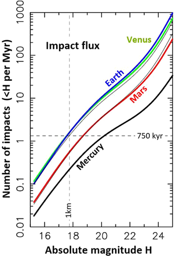
Figure 20. The impact flux on the terrestrial planets as a function of NEO absolute magnitude. The black, green, blue, and red lines show the impact flux for Mercury, Venus, Earth, and Mars. The thin solid lines near the Earth flux are the base-model NEO magnitude distribution scaled with the fixed impact probability (1.5 × 10⁻³ Myr−1; see the main text). The thin solid line near the Mars flux is the Earth profile scaled down by a factor of 3. The horizontal dashed line shows the impact flux for D > 1 km bodies from Morbidelli et al. (2020; 0.75 Myr average spacing between impacts). The vertical dashed line corresponds to H = 17.75.
Download figure:
Standard image High-resolution imageThere are several sources of uncertainty in our impact flux estimates. The first one is related to the uncertainty of the NEO population estimate in Equation (13). As we discussed in Section 6, the relative 1σ uncertainty of our base-model population estimate gradually increases from ≃3% for H < 20 to ≃6% for H < 25. The second source of uncertainty is the uncertainty of the impact fluxes fimp,j for bodies evolving from individual sources (Table 5). This uncertainty varies with source, target planet, and q*. In the best case, we record thousands of impacts on the Earth/Venus from the ν6 resonance for any q*; this would imply a ≲3% uncertainty. In the worst case, for the outer resonances, Mars/Mercury and large q*, there are only a few impacts, but the outer resonances are not important for impacts anyway, so this should not be a major limitation of this work. The third and also the least understood source of uncertainty is related to the detection efficiency of CSS (photometric efficiency and trailing loss, Section 4; Jedicke et al. 2016). We are unable to quantify it here and leave this issue for future work.
Table 6 reports the impact probabilities from different sources for Mercury, Venus, and Mars. We used Equation (13) to compute the total impact flux on these planets as a function of impactor’s absolute magnitude (Figure 20). The impact fluxes on the Earth and Venus are similar. The impact flux on Mercury shows a shallower profile with H mainly because small NEOs on orbits near Mercury are disrupted before they can impact. The size distribution of small (<10 km) craters on young Mercury terrains should be shallower than those found on the Moon and Mars, and this could have interesting applications to the Mercurian chronology as well.
Table 6. Impact Probabilities (pimp) of NEOs from Different Sources
| Source | Mercury | Venus | Earth | Mars |
|---|---|---|---|---|
| % | % | % | % | |
| ν6 | 0.273 | 2.042 | 2.035 | 0.317 |
| 3:1 | 0.035 | 0.227 | 0.273 | 0.041 |
| 5:2 | 0.006 | 0.023 | 0.041 | 0.004 |
| 7:3 | 0.001 | 0.011 | 0.006 | 0.004 |
| 8:3 | 0.015 | 0.099 | 0.138 | 0.067 |
| 9:4 | 0.000 | 0.009 | 0.028 | 0.006 |
| 11:5 | 0.000 | 0.017 | 0.009 | 0.017 |
| 2:1 | 0.001 | 0.013 | 0.010 | 0.006 |
| inner weak | 0.122 | 1.221 | 1.262 | 0.895 |
| Hungarias | 0.258 | 2.266 | 2.802 | 2.001 |
| Phocaeas | 0.069 | 0.708 | 0.666 | 0.388 |
Note. The values are given for the model with the fixed disruption distance q* = 0.1 au. The impact fluxes (fimp) for different planets can be computed by dividing the probabilities given here by the average NEO lifetimes given in Table 5.
Download table as: ASCIITypeset image
7.1. Impact Ratios and the Rb Parameter
The Earth-to-Mars ratio in the number of impacts, E/Ma, is an important parameter often used to transfer the lunar crater chronology to Mars (e.g., Hartmann 2005; Marchi 2021). Here we find E/Ma ≃ 2.8 for H = 15 and E/Ma ≃ 4.3 for H = 25 (Figure 20). Adopting the standard Earth-to-Moon impact flux ratio, E/Mo = 20, we estimate that the Mars-to-Moon ratio in the number of impacts is Ma/Mo ≃ 7.1 for H = 15 and Ma/Mo ≃ 4.7 for H = 25. In crater chronology studies, this is often normalized to the unit surface area on these worlds (Mars has ≃3.8 larger surface area than the Moon), giving the parameter Rb, where the index b stands for bolides. We thus obtain Rb = 2.0 for H = 15 and Rb = 1.2 for H = 25. Both these values are significantly lower than Rb ≃ 2.6 used for NEO impacts in previous works (e.g., Hartmann 2005; Marchi 2021).
The ratio of impact fluxes is size dependent, as a consequence of the size-dependent contribution of different main-belt sources (small and large bodies have different orbital distributions). For small bodies, the ν6 and 3:1 sources dominate, and these resonances have—on their own— Rb ≃ 0.8 (they quickly move asteroids into the NEO zone where they can impact Earth/Moon rather than Mars). For large bodies, the weak resonances are important; they have— on their own—Rb ≃ 2.8 (because asteroids in the weak resonances spend a long time on Mars-crossing orbits and have a greater chance of Mars impact). We emphasize that these estimates accurately account for all impacts, including those from q > 1.3 au. The Rb parameter is relatively low for small impactors, not because we would be missing any Mars impacts from q > 1.3 au. It is low simply because the ν6 and 3:1 resonances give fewer impacts on Mars relative to the Moon.
The method we use here to estimate the Rb parameter is the best we can think of. First, by calibrating the model on NEO observations, we infer the flux of asteroids from different main-belt sources. We already know the impact probability per one body evolving from each source (all planetary impacts were recorded by the N-body integrator; Section 3), and this allows us to accurately estimate the impact flux on the terrestrial worlds. Still, there are some approximations. The main caveat of this method is that we assume that Mars impactors are on unstable orbits (e.g., in strong or diffusive resonances, scattered by Mars) that typically evolve, over long timescales, to q < 1.3 au, and we can therefore calibrate them from NEOs. Our estimates would be inaccurate if many Mars impactors remain on semistable orbits with q > 1.3 au over very long time intervals (longer than our integration time span, 500 Myr). We plan on verifying this assumption in forthcoming work. We also did not account for weak resonances with a > 2.5 au (higher order than 11:5). If these weak resonances were included as an additional source in the model, and the model was recalibrated, then perhaps the weight might (slightly) shift from stronger resonances, such as 5:2 and 8:3, to weaker resonances, and this could influence Rb. In any case, this effect could only change Rb for large, H ≲ 18 asteroids, not the small ones. Full resolution of this problem is left for future work.
Previous estimates of Rb for asteroids were inferred from the Mars-crossing population of large asteroids. For example, Bottke et al. (2002) estimated Rb = 2.8 for H < 18, which is significantly larger than our Rb ≃ 1.8 for H < 18. Bottke et al. (2002) inferred Rb from the Mars-crossing population known in 2002. They accounted for secular variations of Mars’s orbit, computed the impact probabilities on a grid in (a, e, i) space, and approximately compensated for the observational incompleteness. This allowed them to estimate that the mean interval between impacts of H < 18 asteroids on Mars is τMars(18) ≃ 1 Myr, thus giving Rb = 2.8. Here we employed the same method with the asteroid catalog available in 2022. If the cataloged asteroids with q < 1.8 au and H < 18 are assumed to be a complete sample, we find τMars(18) ≃ 2 Myr, some two times longer than reported in Bottke et al. (2002). This would indicate Rb ≃ 1.4. A ≃70% completeness for q < 1.8 au and H < 18 would give Rb ≃ 1.8, in agreement with the estimate inferred from our NEO-based method. To obtain Rb ≃ 2.8 from Bottke et al. (2002), the current population of q < 1.8 au and H < 18 asteroids would have to be only ≃50% complete.
8. Auxiliary Models
To this point we only presented the results of the 28-parameter base model. We now discuss several model modifications to explain some of our choices that we made to assemble the base model. We also explore the model validity beyond the range of parameters considered in the base model.
In the first modification, the base model domain was extended to fainter magnitudes, 15 < H < 28. The modified model produced a reasonable fit to the CSS observations (i.e., relatively large evidence; Figure 21). The extension to fainter magnitudes, however, revealed an intriguing difference relative to the intrinsic (debiased) magnitude distribution given in Harris & Chodas (2021; see also Figure 22). Our distribution is slightly shallower for H > 25 and leads to a smaller population of NEOs with H < 28. Specifically, Harris & Chodas (2021) estimated ≃3.6 × 10⁷ NEOs with H < 28, whereas we have (1.4 ± 0.2) × 107 NEOs with H < 28, a value that is roughly 2.6 times lower (see Section 10.1 for a discussion of constraints from bolide observations). The difference could be explained if we overestimated the CSS detection efficiency for H > 25, perhaps because of some issue with the trailing loss (Section 4.4). Alternatively, some of the assumptions in Harris & Chodas (2021) may not be quite right. Harris & Chodas (2021) did not derive any formal uncertainty of their population estimates, but suggested that their extrapolation to the faintest magnitudes may be up to a factor of ∼5 uncertain. We discuss this issue in Section 10.1.
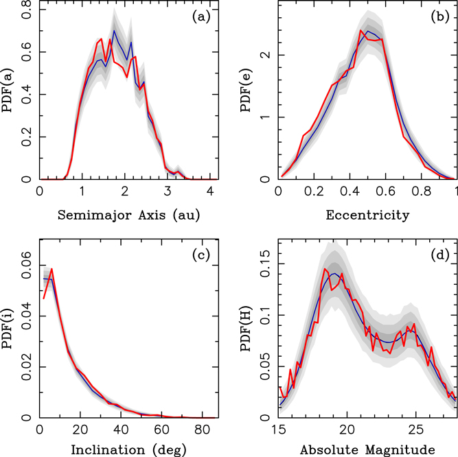
Figure 21. The probability PDFs of a, e, i, and H from our modified base model with the extended magnitude range (15 < H < 28; blue lines) is compared to the CSS NEO detections (red lines). The shaded areas are 1σ (bold gray), 2σ (medium), and 3σ (light gray) envelopes. We used the best-fit solution (the one with the maximum likelihood) from the modified base model and generated 30,000 random samples with 4412 NEOs each (the sample size identical to the number of CSS’s NEOs in the model domain; 15 < H < 28). The samples were biased and binned. We identified envelopes containing 68.3% (1σ), 95.5% (2σ), and 99.7% (3σ) of samples and plotted them here.
Download figure:
Standard image High-resolution image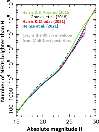
Figure 22. The (intrinsic) absolute magnitude distribution from the modified base model where we extended the model domain to 15 < H < 28 (solid black line). The gray area shows the 99.7% envelope of posteriors from the MultiNest fit. For reference, we also plot the magnitude distributions from Harris & D’Abramo (2015; green line), Granvik et al. (2018; dashed black line for 17 < H < 25), Harris & Chodas (2021; red line), and Heinze et al. (2021; blue line). Note that the vertical blue bar at H = 28 shows the 1σ uncertainty reported in Heinze et al. (2021) for the number of NEO with H < 28.
Download figure:
Standard image High-resolution imageThe absolute magnitude distribution given in Table 6 of Granvik et al. (2018) has a shape similar to ours but indicates a somewhat larger population of NEOs (Figure 22). The difference is statistically significant. For example, Granvik et al. (2018) estimated (8.02 ± 0.45) × 105 NEOs with H < 24.875, while we only have (3.4 ± 0.2) × 105 NEOs with H < 24.875 (1σ uncertainties quoted here). Our estimates for H < 25 closely agree with those given in Heinze et al. (2021). Heinze et al. (2021) estimated (3.72 ± 0.49) × 105 NEOs with H < 25 while we only have (3.6 ± 0.2) × 105 NEOs with H < 25 (Table 4). For 25 < H < 28, the magnitude distribution given in Heinze et al. (2021) is similar to that of Harris & Chodas (2021) but steeper than ours (Figure 22). This leads to (2.64 ± 0.88) × 107 NEOs with H < 28 in Heinze et al. (2021) and (1.4 ± 0.1) × 107 NEOs with H < 28 here. Given the relatively large uncertainty in Heinze et al. (2021), however, this difference is not statistically significant (only ≃1.4 σ).
In the second modification, we kept the extended magnitude range (15 < H < 28), and used the trailing loss from Tricarico (2017; see also Section 4.4). In this case, the intrinsic magnitude distribution of model NEOs again closely follows Harris & Chodas (2021) to about H = 25. A relatively large difference then appears for fainter magnitudes, where the modified model gives a very shallow slope and only (8.9 ± 0.9) × 106 NEOs with H < 28. This is a factor of ≃4 below the estimate of Harris & Chodas (2021), and a factor of ≃1.6 below the estimate obtained above with the trailing loss from Zavodny et al. (2008). This may indicate that the trailing loss from Tricarico (2017) overestimates the CSS detection efficiency for very faint NEOs. In broader sense, this highlights the dependence of the population estimates obtained here for very faint NEOs on the adopted trailing loss model.
In the third modification, we used the trailing loss from Zavodny et al. (2008), but did not fix N(15) = 50. Instead, we let the MultiNest fit decide what the population of H < 15 should be based on the CSS data for H > 15. If N(15) is not fixed, the model overestimates, by roughly a factor of 2, the number of NEOs brighter than H = 15. This most likely happens because the statistical power of the brightest CSS NEOs in the MultiNest fit is not great enough to properly fix N(15). We therefore impose N(15) in the base model as an external constraint (Section 6).
We also tested a slight modification of the fitting procedure, where G96 and 703 were treated as separate surveys. The log-likelihood in Equation (8) was computed separately for them, and was subsequently combined to evaluate the total log-likelihood. Strictly speaking, combining the surveys at the level of log-likelihoods must be better than combining their detection efficiencies and object detections. This is because the detection bias of the G96 survey only applies to NEO detections in the G96 survey (and not 703), and vice versa. Note that this method is different from testing the two surveys separately; it makes use of the full statistical power of them combined.
The results of this test were similar to those obtained with the standard method, but we also noted several differences. The contribution of the ν6 resonance to NEOs with H = 15 is smaller than that reported in Table 3 (here  ). This can indicate that—at least for some parameters—the systematics in the model fitting may be the dominant source of uncertainties, and some source weights may be more uncertain than indicated in Table 3. The differences for all other source weights and other parameters are smaller than 30%. For some reason, the new fitting procedure also gives N(17.75) = 1010 ± 19—an ∼8% larger population than that obtained in the base model (and smaller uncertainty). This indicates that an accurate population estimate (also) depends on the details of the fitting algorithm. A detailed investigation of this approach is left for future work. Our preliminary results from 2013–2021 CSS observations, for which we derived the CSS detection efficiency from scratch (Nesvorný et al. 2023, in preparation), favor combining surveys at the level of log-likelihoods and indicate N(17.75) = 931 ± 21. It thus appears that the detection efficiency of the original CSS for H < 17.75 was slightly underestimated (Jedicke et al. 2016), and this was compensated for by combining the detection efficiencies of G96 and 703 (Granvik et al. 2018).
Following Granvik et al. (2016), our base model accounted for the size-dependent disruption of NEOs at low perihelion distances. We extensively tested various NEO models where the disruption module in MultiNest was switched off. All modified models without disruption showed a strong excess of high–e and low–q orbits, and Bayes factors that strongly disfavored them ( in favor of the base model). We also tested several models where the disruption module in MultiNest was switched on, but the dependence of q* on H was ignored (i.e., fixed q* for all sizes). Again, the evidence term showed a strong preference for the models with the size-dependent disruption (
 in favor of the base model). This confirms the results of Granvik et al. (2016).
9. Models with the Yarkovsky Drift
The methodology described above, where the contribution of different main-belt sources is inferred from the NEO population, is agnostic as to whether the main-belt sources can actually provide that contribution. This depends on the influx of main-belt asteroids into resonant sources and complex interaction of drifting orbits with weak resonances in the inner belt and for the Hungarias and Phocaeas. To test this, we performed new numerical integrations in which bodies were not placed onto unstable orbits in the resonances. Instead, we collected real main-belt asteroids near a resonance, accounted for the Yarkovsky effect (Vokrouhlický et al. 2015), and followed bodies as they drifted into the resonance and became NEOs. Two cases were considered: one with the maximum (theoretically possible) Yarkovsky drift, and one where the drift was set to the mean (theoretically estimated) Yarkovsky rate. In either case, asteroids were assumed to drift toward the resonance. The first case maximizes the asteroid flux into the source. The second case would correspond to a situation where asteroids drift toward the resonance with random obliquities.
Adopting thermal parameters appropriate for the S- and C-type asteroids (Vokrouhlický et al. 2015), we estimate that the maximum Yarkovsky drift of a reference D = 1 km body at a = 2.5 au is  au Myr−1 for S, and
  au Myr−1 for C. For comparison, if the measured Yarkovsky drifts for Golevka (S-type) and Bennu (C-type) are rescaled to the same size and orbital radius, we obtain 2.25 × 10⁻⁴ au Myr−1 and 1.82 × 10⁻⁴ au Myr−1, respectively (Greenberg et al. 2020). Given these results, we decided to make no distinction between S- and C-type asteroids, and adopted the drift rate
where θ is the asteroid obliquity.
We considered all main-belt asteroids near the 3:1 resonance that could potentially drift into the resonance in 100 Myr. Near the 3:1 resonance, the maximum accumulated drift of a D = 1 km body over 100 Myr is ≃0.02 au. We therefore set, with a generous safety margin, a1(e) = 2.46 − (0.02/0.35)e au and a2(e) = 2.54 + (0.02/0.35)e au, and collected all known main-belt asteroids with H < 17.75, q > 1.66 au and a1(e) < a < a2(e) (31,121 in total). The numerical integrations were performed with the modified Swift integrator, where artificial force terms were added to account for da/dt from Equation (14). The diameters in Equation (14) were estimated from the absolute magnitudes of selected asteroids and the reference albedo pV = 0.14. The orbits of eight planets and all selected asteroids were integrated with a 12 daytime step for 100 Myr.
In the case with the maximum drift rate, we set θ = 0 for a < 2.5 au and θ = 180° for a > 2.5 au. We found that η = 11,107 asteroids reached the NEO region in 100 Myr. The number of NEOs expected from this influx in a steady state is η τ/(100 Myr) where τ is the mean NEO lifetime for objects evolving from the 3:1 source (Table 5). For q* = 0–0.1 au, which should be appropriate for H < 17.75 (Figure 15), we have τ = 1.4–2.5 Myr. We can thus estimate that the 3:1 resonance should contribute ≃155–277 NEOs with H < 17.75. This is roughly consistent with the result of Morbidelli & Vokrouhlický (2003), who found, in the case where the effects of YORP and collisions were suppressed, ≃161 H < 18 NEOs from 3:1. For comparison, we inferred from the base model in Section 6 that the 3:1 source should produce ≃24% ± 4% of NEOs with H < 17.75 (Figure 14). This gives ≃180–268 NEOs for N(17.75) = 931 ± 30 (Section 6). We conclude that the model with the maximum Yarkovsky drift of large main-belt asteroids toward the 3:1 resonance is consistent with what is needed from the NEO-population modeling (Section 6).
The same simulations were repeated with the mean Yarkovsky drift toward the 3:1 resonance (the mean rate is one-half of the maximum rate for random orientation of the spin axes; Vokrouhlický et al. 2015), and found η ≃ 5 000. This case can be ruled out because it only gives ≃70–124 NEOs with H < 17.75. Given these results, the case with fully random obliquities, where the main-belt asteroids would drift toward or away from the 3:1 resonance, was not investigated in detail; we roughly estimate that this case would only give <70 NEOs with H < 17.75.
We conclude that asteroids near the 3:1 resonance must be drifting toward the resonance with the (near) maximum Yarkovsky drift rates (≃2 × 10⁻⁴ au Myr−1 for D = 1 km). This most likely happens because large, slow-drifting asteroids cannot cross the 3:1 resonance, and this produces a dynamical bias, where all asteroids currently in the immediate neighborhood of the 3:1 resonance must be drifting toward it. In addition, the YORP effect must have driven their obliquities to θ ≃ 0 or θ ≃ 180°, and this maximized the Yarkovsky drift and resonance feeding rate.
This result has several interesting consequences. First, in the immediate neighborhood of the 3:1 resonance, ∼kilometer-class asteroids should have θ ≃ 0 for a < 2.5 au and θ ≃ 180° for a > 2.5 au. This prediction is testable by light-curve observations (see the note at the end of the main text). Second, the spin reorientation timescale of ∼kilometer-class main-belt asteroids via collisions or YORP (Vokrouhlický et al. 2015) should be relatively long. As bodies keep their drift directions, they must be drifting toward the resonance and not away from it; the bodies currently drifting away from the resonance would have to have a relatively recent (<100 Myr) reorientation event. Third, the YORP effect must have driven obliquities of kilometer-class bodies to either θ ≃ 0 or θ ≃ 180°. This rules out, on the population level, the YORP models/shapes that lead to θ ∼ 90° and sets limits on the importance of spin–orbit resonances (Vokrouhlický et al. 2003, 2006).
Similar tests were performed for the ν6 and 5:2 resonances. For the 5:2 resonance, we found η = 10,169—the influx in the 5:2 resonance is thus similar to the influx in the 3:1 resonance. We estimate ≃31–46 NEOs with H < 17.75 from 5:2 in the steady state. For comparison, our NEO model nominally implies ≃56 NEOs from the 5:2 source, but this value has a relatively large uncertainty (Table 3) and is consistent within 1σ with the drift-inferred values. In addition, the population of H < 17.75 main-belt asteroids near the 5:2 resonance is probably incomplete, which may account for some of the difference as well. For the ν6 resonance, where da/dt < 0 was assumed for all orbits, we found a lower influx, η = 4 040, because the region adjacent to the ν6 resonance is sparsely populated. With the relatively long lifetimes of orbits evolving from ν6 (Table 5), this implies ≃237–318 NEOs with H < 17.75, to be compared with ≃186 inferred in Section 6 for the ν6 source. An accurate comparison is somewhat complicated in this case because many asteroids in the drift simulations reached the NEO orbits via weak resonances, and not from ν6.
The simulations presented here offer an opportunity to test whether the NEO orbital distributions obtained from different sources sensitively depend on the initial conditions. The model described in Section 6 was based on the orbital distributions obtained from the simulations where test bodies were inserted onto unstable orbits in resonances. Here we instead drifted real main-belt asteroids into resonances. We can therefore compare the orbital distributions of NEOs obtained from the two methods to see if there are any important differences. We find that the distributions obtained from the two methods are practically identical (<1% differences for ν6, 3:1, and 5:2). This justifies our preferred approach to this problem described in Section 5.1.
10. Discussion
10.1. Magnitude Distribution of NEOs
Harris & Chodas (2021) determined the absolute magnitude distribution of NEOs by comparing detections of new NEOs with redetections of previously known NEOs (also see Harris & D’Abramo 2015). If all objects were equally detectable, the ratio of new detections to redetections in a survey is proportional to the number of not yet discovered NEOs, thus giving clues about the observational incompleteness. Given that the observational bias is the same for both the new detections and redetections, by using the ratio of the two, the method is relatively insensitive to the observational bias, and different surveys can be clumped together to improve the statistics. Harris & Chodas (2021) approximately accounted for observational biases of different surveys to correct the estimates for unequal detectability of NEOs on different orbits. They also corrected a small error in Harris & D’Abramo (2015) related to a rounding problem.
The method based on redetections is limited to a magnitude range where the numbers of new detections and redetections are statistically large, which, according to Harris & D’Abramo (2015), corresponds to the magnitude range 17.5 < H < 23.5. To extrapolate the results to fainter magnitudes, where there are no or too few redetections, Harris & D’Abramo (2015) and Harris & Chodas (2021) assumed that a survey detects an increasingly smaller fraction of the NEO population and estimated—from the statistics of close encounters of faint NEOs to the Earth—that this fraction is proportional to 10−0.8H . Finally, anchoring the results to the re-detection ratio approach at H ≃ 23.5, they produced the absolute magnitude distribution of NEOs for 25 ≤ H ≤ 31.
To demonstrate the applicability of their estimate, Harris & Chodas (2021) used the fixed impact flux probability with the Earth, fimp = 1.5 × 10⁻³ Myr−1, for each NEO, and compared their impact statistics with that inferred from observations of bolides (Brown et al. 2002). Brown et al. (2002) analyzed satellite records of bolide detonations in the Earth atmosphere to estimate the impact flux of ∼1–10 m bodies. For D ≃ 10 m, roughly equivalent to H = 28 for our reference albedo pV = 0.14, the average interval between impacts was found ≃10 yr (with a factor of ≃2 uncertainty). The infrasound data from Silber et al. (2009), as reported by Brown et al. (2013), indicate a somewhat shorter interval, but the error bars of these estimates overlap with the bolide data. For comparison, Harris & Chodas (2021) estimated the average interval between impacts of H < 28 bodies to be ≃18 yr (Figure 23).
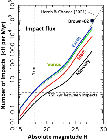
Figure 23. The impact flux on the terrestrial planets as function of NEOs absolute magnitude. The black, green, blue, and red lines show the impact flux for Mercury, Venus, Earth, and Mars, respectively, from Equation (13). The thin solid line near the Earth flux is the NEO magnitude distribution from Harris & Chodas (2021) scaled with the fixed impact probability (1.5 × 10⁻³ Myr−1; see the main text). The black dot approximately marks the constraint from bolide detonations in the Earth atmosphere (Brown et al. 2002). The horizontal dashed line shows the impact flux for D > 1 km bodies from Morbidelli et al. (2020; 0.75 Myr average spacing between impacts). The vertical dashed line corresponds to H = 17.75.
Download figure:
Standard image High-resolution imageHere we find that the magnitude distribution is relatively shallow for H > 25 and estimate a somewhat smaller population of faint NEOs (Section 8). We also find, however, that the Earth-impact probability of faint NEOs is relatively large (because they evolve onto NEO orbits via the ν6 resonance), and that this larger impact probability at least partially compensates for the smaller population. For example, we have fimp ≃ 1.5 × 10⁻³ Myr−1 for H = 15 and fimp ≃ 2.6 × 10⁻³ Myr−1 for H = 28. The mean interval between impacts for H < 28 is estimated here to be ≃30 yr (Figure 23). This is factors of 1.6 and 3 longer than the nominal intervals from Harris & Chodas (2021) and Brown et al. (2002, 2013), respectively. Adopting our estimate, the probability of having four impacts in the last 30 yr from D > 10 m projectiles would only be 1.5%. Brown et al. (2013) suggested that the current impactor flux for near-Earth asteroids that are 10–50 m in diameter may be higher than the long-term average.
Note that all estimates quoted above have significant uncertainties. Brown et al. (2002, 2013) reported a factor of ≃2 uncertainty in their estimates from bolide and infrasound observations, but the fact that these two estimates agree means that the combined uncertainty would be smaller. Harris & Chodas (2021) suggested a factor of few uncertainty in their estimate. Our impact flux estimate is at least ≃10% uncertain (1σ from the magnitude distribution uncertainty for H = 28; Figure 22) and probably much more given that we were not able to characterize the uncertainty of the CSS detection efficiency (Section 4). It is possible, for example, that the CSS detection efficiency is overestimated by a factor of ≃2–3 for H ≃ 28. If so, this would bring our impact flux up by the same factor. It is also possible that the difference between our estimates and bolide/infrasound data has some interesting physical explanation. We are testing different possibilities and will report on the results in forthcoming publications.
10.2. PM/AM Ratio
There has been some debate about the PM/AM ratio of meteorites/bolides (Morbidelli & Gladman 1998; Wisdom 2017, 2020). The PM/AM ratio measures the relative frequency of meteorite falls before (6–12 hr) and after (12–18 hr) noon. It is usually reported as the number of afternoon falls (12–18 hr) over the number of daytime falls (6–18 hr), to express the observed excess of afternoon falls, here denoted as  . Ordinary chondrites (OCs), for example, have
  (Wisdom 2017). Morbidelli & Gladman (1998) obtained
  and 0.48 for impactors from the ν6 and 3:1 resonances, respectively (no cutoff on collisional lifetime or entry velocity imposed here), and suggested that the PM excess of reported OC falls should be a consequence of the collisional removal of meteoroids (young NEOs tend to have a stronger PM excess). Wisdom (2020), as an update on Wisdom (2017), estimated
  and 0.604 ± 0.007 from the ν6 and 3:1 resonance, respectively. He argued that the previous (lower) estimates of Morbidelli & Gladman (1998) were wrong because—to calculate
  —Morbidelli & Gladman (1998) incorrectly assumed orbits with a uniformly random distribution of the argument of perihelion, ω.
Here we take the opportunity to rectify this issue. Our N-body integration recorded a large number of Earth impacts from bodies started in the ν6 (2527 in total) and 3:1 resonances (398 in total). For each impact, we propagated the impactor to the Earth’s surface and determined the geocentric coordinates of the impact. This allowed us to estimate  without any uncertainty related to the ω distribution. The nighttime impacts were ignored. To be consistent with the previous work (Morbidelli & Gladman 1998; Wisdom 2017, 2020), the Earth obliquity was neglected in this test.
We obtained  and 0.50 ± 0.05 for the ν6 and 3:1 resonances, respectively. These values are better aligned with Morbidelli & Gladman (1998) than with Wisdom (2017, 2020). The PM excess reported in Wisdom (2017) for the 3:1 resonance is roughly 2σ above our value. The reasons behind this are uncertain. Part of the difference may be explained by the relatively short integration time span (20 Myr in Wisdom 2017, 2020). When the integrations were extended to 40 Myr, Wisdom (2020) found
  for the 3:1 resonance. Here we find the same trend: the early impacts show higher PM excess than the late ones (e.g.,
  from the 3:1 resonance and t < 10 Myr).
For reference, we also computed the PM excess with the disruption model (Section 5.3). For example, for q* = 0.3 au, which should be appropriate for 1–10 m meteoroids, we find  and 0.58 ± 0.08 for the ν6 and 3:1 resonances. Meteoroid disruption close to the Sun can thus significantly influence the PM excess. The observed statistics of PM/AM falls shows higher excess (
 ) than the values derived here for the ν6 and 3:1 resonances. Morbidelli & Gladman (1998) suggested that the excess increases in the model when it accounts for the collisional lifetime of meteoroids. A possible solution to this problem could thus be that the PM excess is influenced by the physical lifetime of meteoroids (collisional disruption, disruption at low perihelia, YORP spin-up, etc.)
10.3. Size Dependencies
The size-dependent sampling of main-belt sources found here, both in terms of their contribution to the NEO population and Earth impacts, helps to resolve the following scientific problem. Granvik et al. (2018) estimated that the outer-belt contribution to NEOs is practically negligible (≃3.5% for the 2:1 resonance complex). They suggested that ≃80% of impactors on the terrestrial worlds are produced from the ν6 resonance, and over 10% of impactors are produced from the 3:1 resonance, Hungarias and Phocaeas, leaving only <10% for the middle/outer belt. Based on this, Granvik et al. (2018) proposed that the majority of primitive NEOs/impactors must come from the ν6 resonance. Nesvorný et al. (2021) instead found that the middle/outer belt can supply nearly 50% of large NEOs, ≃70% of large primitive NEOs, and ≃35%–40% of large impactors (D ≳ 5 km).
Nesvorný et al. (2021) speculated that these differences may be a consequence of the size-dependent delivery process. On one hand, small main-belt asteroids can drift over a considerable radial distance by the Yarkovsky effect and reach NEO space from the powerful ν6 resonance at the inner edge of the asteroid belt (e.g., Granvik et al. 2017). The ν6 resonance is known to produce highly evolved NEO orbits and high impact probabilities on the Earth (Table 6; Gladman et al. 1997). On the other hand, large main-belt asteroids often reach NEO orbits via slow orbital evolution in weak resonances (Migliorini et al. 1998; Farinella & Vokrouhlický 1999; Morbidelli & Nesvorný 1999). Whereas each of these resonances adds only a small amount, their total contribution to the population of large NEOs can be significant.
Here we find supporting evidence for this thesis. For H = 15 (D = 3.5 km for the reference albedo pV = 0.14), we find that the middle/outer main belt produce ≃40% of NEOs. When extrapolated to D > 5 km, this should be consistent with the similarly large contribution reported in Nesvorný et al. (2021). For H = 25 (D = 35 m for a reference albedo pV = 0.14), however, the contribution is only ≃10% (the 3:1 source is excluded here). The ν6 and 3:1 resonances produce ≃80% of small NEOs for H = 25 (and ≃90% of small Earth impactors; Section 7), which is in line with the findings reported in Granvik et al. (2018).
11. Summary
The main results of this work are summarized as follows.
- 1.We developed a new NEO model (NEOMOD). The model is based on numerical integrations of bodies from 12 sources (11 main-belt sources and comets). A flexible method to accurately calculate biases of NEO surveys was applied to CSS observations from 2005–2012 (Christensen et al. 2012). The MultiNest code (Feroz & Hobson 2008; Feroz et al. 2009) was used to calibrate the model on CSS detections. The algorithms developed here can be readily adapted to any current or future NEO survey.
- 2.The methodology used in Granvik et al. (2018) was improved. We adopted the cubic splines to characterize the magnitude distribution of the NEO population. The cubic splines are flexible and can be modified to consider a broader absolute magnitude range and/or improve the model accuracy. We used a large number of main-belt asteroids in each source (105), which allowed us to accurately estimate the impact fluxes on the terrestrial planets. Our model self-consistently accounts for the NEO disruption at small perihelion distances (Granvik et al. 2016).
- 3.We used 10,000 test objects per orbital bin, 18,480 orbital bins, 56 absolute magnitude bins, and nearly 250,000 FOVs to compute the CSS detection probability as a function of NEO’s a, e, i, and H. We considered different approaches to modeling the trailing loss of CSS. The trailing loss represents an important uncertainty in estimating the population of small NEOs, and we urge surveys to carefully characterize it.
- 4.Our base model is available via the NEOMOD Simulator (Section 6), a code that can be used to generate a user-defined sample of model NEOs. Researchers interested in the probability that a specific NEO evolved from a particular source can obtain this information from the ASCII table that is available along with the Simulator. Optionally, the NEOMOD Simulator can output the information about the impact probability of model-generated NEOs with the Earth.
- 5.We found that the sampling of main-belt sources by NEOs is size-dependent, with the ν6 and 3:1 resonances contributing ≃30% of NEOs with H = 15, and ≃80% of NEOs with H = 25. This trend most likely arises from how the small and large main-belt asteroids reach the source regions. The size-dependent sampling suggests that small terrestrial impactors preferentially arrive from the ν6 source, whereas the large impactors can commonly come from the middle/outer belt (Nesvorný et al. 2021).
- 6.We confirm the size-dependent disruption of NEOs reported in Granvik et al. (2016), and find a similar dependence of the disruption distance on the absolute magnitude. As a consequence of the size-dependent disruption and item (5), small and large NEOs have different orbital distributions.
- 7.Although the base NEOMOD fit only applies to H < 25, the fit in the extended magnitude range shows a shallower absolute magnitude distribution for 25 < H < 28 and smaller number of NEOs with H < 28 than that of Harris & Chodas (2021). The average time between terrestrial impacts of D ≃ 10 m bolides is found to be ≃30 yr—≃3 times longer than the nominal estimate from Brown et al. (2002, 2013). These differences may point to some problem with the detection efficiency of CSS for 25 < H < 28. Alternatively, they may have some interesting physical explanation.
- 8.We compute the PM excess of meteorite falls for meteoroids evolving from the ν6 and 3:1 resonances to find
 and 0.50 ± 0.05, respectively. These values are better aligned with Morbidelli & Gladman (1998) than with Wisdom (2017, 2020). The observed statistics of PM/AM falls shows higher excess () than the values derived here for the ν6 and 3:1 resonances. The PM excess can be influenced by the physical lifetime of meteoroids.
 - 9.The model-inferred contribution of the 3:1 source to large NEOs (H ≲ 18) implies that the main-belt asteroids should drift toward the 3:1 resonance at the maximum Yarkovsky drift rates (≃2 × 10⁻⁴ au Myr−1 for a ≃1 km diameter body at 2.5 au). This suggests that the main-belt asteroids on the sunward side of the 3:1 resonance (a < 2.5 au) have obliquities θ ≃ 0°; those with a > 2.5 au should have θ ≃ 180° (in the immediate neighborhood of the resonance). A similar inference applies to the ν6 and 5:2 resonances (it should apply to other resonances as well). These predictions are testable from light-curve observations.
- 10.The contribution of inactive comets to the NEO population is inferred to be smaller than in previous works (αJFC < 0.017; 68.3% envelope). For comparison, Bottke et al. (2002) found a ≃6% contribution of JFCs, and Granvik et al. (2018) suggested a 2%–10% H-dependent contribution. As the Bayes factor slightly favors a model without any comet contribution, the evidence for cometary NEOs can thus be hard to extract from the CSS observations alone. This may imply that JFCs disrupt rather than becoming dormant (see Nesvorný et al. 2010).
- 11.We estimate that the Mars-to-Moon ratio in the number of impacts is Ma/Mo ≃ 7.1 for H = 15 and Ma/Mo ≃ 4.7 for H = 25. In crater chronology studies, this is often normalized to the unit surface area on these worlds, giving the parameter Rb, where the index b stands for bolides. We obtain Rb = 2.0 for H = 15 and Rb = 1.2 for H = 25. Both of these values are significantly lower than Rb ≃ 2.6 used for NEO impacts in previous works.


Ďurech & Hanuš (2022, private communication) recently analyzed the Gaia data release 3 (DR3) to determine the obliquities for ≃9500 asteroids. The distribution of obliquities confirms the trend predicted in Section 8 and item (9) above. The obliquities of main-belt asteroids immediately sunward of strong orbital resonances are θ < 90°, with a concentration for θ < 45°; capture in spin–orbit resonances is probably important here. The obliquities on the opposite side of resonances are θ ≃ 180°, exactly as predicted here to produce sufficiently large feeding rates.
Acknowledgments
The simulations were performed on the NASA Pleiades Supercomputer. We thank the NASA NAS computing division for continued support. The work of D.N., R.D., and W.F.B. was supported by the NASA Planetary Defense Coordination Office project “Constructing a New Model of the Near-Earth Object Population.” The work of S.N., S.R.C., and P.W.C. was conducted at the Jet Propulsion Laboratory, California Institute of Technology, under a contract with the National Aeronautics and Space Administration. D.V. acknowledges support from the grant 21-11058S of the Czech Science Foundation. We thank an anonymous reviewer for helpful comments.
Footnotes
- 13
- 14
- 15
The double Gaussian distribution is given here by
- 16
The cloning consisted of applying a 10−6 relative change to the velocity vector of each object.
- 17
The optimal time step was determined by convergence studies. The results with 12 and 18 hr time steps, both in terms of the orbital distribution produced from different sources and planet impact statistics, were found to be practically identical. Long time steps in excess of 1 day generate artifacts in the orbital distribution of NEOs with short orbital periods. Granvik et al. (2018) used a 12 hr time step as well.
- 18
Note that, as there are many more bins that known NEOs (Section 4), most bins do not contain a known NEO.
- 19
Intentional redetections (e.g., the same object targeted multiple times) have no information content for our work. Accidental redetections of the same object typically happen when the object is relatively bright. The accidental redetections could thus improve the statistics for bright objects.
- 20
More accurately, this applies to a set of four FOVs with the same pointing direction taken by CSS in short succession on the same night (FOV set or “frame”). The detection probability is the probability that the CSS pipeline picks up an object in at least three of these four FOVs. Objects identified in less then three FOVs by the CSS pipeline are not reported as detected.
- 21
- 22
- 23
- 24
- 25
- 26
- 27
More accurately, we should use the binomial distribution with the model-estimated probability of detection in the CSS FOV set given by p = λj /Nimg, where Nimg = 226, 824 is the total number of CSS FOVs. The Poisson distribution should be an adequate approximation of the binomial distribution as long as Nimg is large enough and λj is small enough. Both of these conditions appear to be satisfied in the present case.
- 28
Initially, we sectioned the magnitude range 15 < H < 25 evenly by having four intervals H = 15–17.5, 17.5–20, 20–22.5, and 22.5–25, and found that the use of splines led to a substantial improvement of fits relative to those obtained with the third-order polynomial. The results further improved when the division between the third and fourth intervals was set at H = 24 (instead of 22.5). This is related to the asymmetry of the underlying distribution, which is reproduced slightly better when the third and fourth segments have unequal lengths.
- 29
- 30
- 31
Note that the residence time distribution from ν6 and inner resonances are similar but not equal; the degeneracy between these two sources is therefore not absolute. The inner resonances show the orbital distribution more peaked for a > 2 au, whereas ν6 produces more evolved orbits with a < 2 au.
- 32
- 33
- 34
The ν6, inner weak and 3:1 resonances jointly contribute to ≃54% of H = 15 NEOs.
- 35
See https://www.boulder.swri.edu/~davidn/NEOMOD_Simulator for a provisory distribution.
- 36
Note that the NEO population is used here to calibrate the model, but the impact statistics inferred from this calibration accounts for impactors with q > 1.3 au as well. This is because the N-body integrator recorded all planetary impacts, including those from q > 1.3 au.