Abstract
In 2017, the California-Kepler Survey (CKS) published its first data release (DR1) of high-resolution optical spectra of 1305 planet hosts. Refined CKS planet radii revealed that small planets are bifurcated into two distinct populations, super-Earths (smaller than 1.5 R⊕) and sub-Neptunes (between 2.0 and 4.0 R⊕), with few planets in between (the “radius gap”). Several theoretical models of the radius gap predict variation with stellar mass, but testing these predictions is challenging with CKS DR1 due to its limited M⋆ range of 0.8–1.4 M⊙. Here we present CKS DR2 with 411 additional spectra and derived properties focusing on stars of 0.5–0.8 M⊙. We found that the radius gap follows Rp ∝ Pm with m = −0.10 ± 0.03, consistent with predictions of X-ray and ultraviolet- and core-powered mass-loss mechanisms. We found no evidence that m varies with M⋆. We observed a correlation between the average sub-Neptune size and M⋆. Over 0.5–1.4 M⊙, the average sub-Neptune grows from 2.1 to 2.6 R⊕, following  with α = 0.25 ± 0.03. In contrast, there is no detectable change for super-Earths. These M⋆–Rp trends suggest that protoplanetary disks can efficiently produce cores up to a threshold mass of Mc, which grows linearly with stellar mass according to Mc ≈ 10 M⊕(M⋆/M⊙). There is no significant correlation between sub-Neptune size and stellar metallicity (over −0.5 to +0.5 dex), suggesting a weak relationship between planet envelope opacity and stellar metallicity. Finally, there is no significant variation in sub-Neptune size with stellar age (over 1–10 Gyr), which suggests that the majority of envelope contraction concludes after ∼1 Gyr.
Original content from this work may be used under the terms of the Creative Commons Attribution 4.0 licence. Any further distribution of this work must maintain attribution to the author(s) and the title of the work, journal citation and DOI.
1. Introduction
The key legacy of NASA’s Kepler mission is its sample of over 4000 extrasolar planets. These planets were discovered from precise, nearly continuous photometry obtained over 4 yr of roughly 200,000 stars. Importantly, the Kepler planet population covers a wide range of sizes and orbital periods; sizes range from super-Jupiter to sub-Mercury, and orbital periods extend from less than a day to more than a year (Thompson et al. 2018). The Kepler exoplanet census has, and will continue to, shed light on the diverse outcomes of planet formation.
The distribution of Kepler planets encodes key aspects of planet formation physics, including the growth of solid cores, the accretion (and loss) of gaseous envelopes, and the prevalence of orbital migration. Gaining insights into these processes requires detailed knowledge of host stars. Until 2017, the properties of the vast majority of Kepler planet host stars were based on broadband photometry, which limited the accuracy of star and planet properties. Importantly, photometric stellar radii R⋆ were uncertain at the ∼40% level (Brown et al. 2011).
To address these limitations, our group conducted the California-Kepler Survey (CKS; Petigura et al. 2017), a spectroscopic survey of 1305 planet-hosting stars observed by Kepler (technically Kepler Objects of Interest, or KOIs). The CKS consisted of several overlapping samples, the largest of which was magnitude-limited and included 960 planet hosts brighter than Kepler-band magnitude mKep = 14.2. Using these spectra, we measured Teff,  , and [Fe/H] and refined stellar M⋆, R⋆, and age, along with planet size Rp
and incident stellar flux Sinc.
, and [Fe/H] and refined stellar M⋆, R⋆, and age, along with planet size Rp
and incident stellar flux Sinc.
The CKS stellar properties enabled several insights into the occurrence and properties of planets as a function of stellar metallicity (Petigura et al. 2018b), stellar age (Berger et al. 2018a), planet multiplicity (Weiss et al. 2018), stellar obliquity (Winn et al. 2017), and other properties. One such insight flowed directly from the improvement in R⋆ errors from 40% to 10%: the radius distribution of small planets is bimodal (Fulton et al. 2017). This result has been confirmed in samples of planets with even smaller radius uncertainties that have leveraged asteroseismic or parallax constraints (Berger et al. 2018b; Fulton & Petigura 2018; Van Eylen et al. 2018; Petigura 2020).
This radius gap was predicted by several groups who considered the effect of photoevaporation on planetary envelopes by X-ray and extreme-ultraviolet (XUV) radiation (Lopez & Fortney 2013; Owen & Wu 2013; Jin et al. 2014; Chen & Rogers 2016). Other processes that inject energy into planet envelopes may also produce the gap, such as the luminosity from cooling cores (Ginzburg et al. 2018; Gupta & Schlichting 2019) or the heat from accreting planetesimals (Chatterjee & Chen 2018; Zeng et al. 2019; Wyatt et al. 2020).
Projecting the planet population along the axis of stellar mass should help illuminate which processes sculpt the distribution of small planets. For example, photoevaporation models predict that small planets will lose their envelopes out to lower bolometric flux levels around low-mass stars due to increased FXUV/Fbol.
Such studies are challenging with CKS DR1 because it spans a limited range of M⋆ ≈ 0.8–1.4 M⊙. There are several reasons for this: (1) the Kepler selection function favored FGK stars (Batalha et al. 2010), (2) most of the Kepler stars below 0.8 M⊙ are fainter than mKep = 14.2, and (3) the spectroscopic techniques used in Petigura et al. (2017) could not return reliable parameters for stars cooler than Teff = 4700 K. Despite the limited M⋆ range, analyses of this data set indicated an increase in the average size of sub-Neptunes with increasing stellar mass (Fulton & Petigura 2018; Petigura 2020). In addition, Wu (2019) and Berger et al. (2020b) found a positive M⋆–Rp correlation for sub-Neptunes.
The Teff > 4700 K boundary in CKS poses an additional challenge for interpreting trends with M⋆. This boundary corresponds to M⋆ > 0.65 and 0.80 M⊙ at [Fe/H] = −0.4 and +0.4 dex, respectively, the upper and lower ends of the CKS metallicity distribution. Owen & Murray-Clay (2018) discussed how this correlation acts as a confounding factor for interpreting both mass and metallicity trends in CKS DR1.
Here we present a follow-up survey designed to expand the stellar-mass range of the CKS sample. We constructed a sample of planet hosts spanning 0.5–1.4 M⊙ (Section 2) and gathered Keck/HIRES spectra of those absent from CKS DR1. New spectra of 411 hosts are presented here as CKS DR2 (Section 3). We analyzed the combined DR1/DR2 samples to derive temperatures, metallicities, and limits on stellar companions, which we combined with astrometric and photometric measurements to derive stellar masses, radii, and ages (Section 4). With updated stellar properties, we refined the precision and purity of the planet catalog (Section 5). We analyzed both the distribution of detected planets (Section 6) and the underlying occurrence rate (Section 7). We offer some comparisons to planet formation theory (Section 8) and provide a brief summary and conclusion (Section 9).
2. Sample Selection
Our main goal was to measure planet occurrence as a function of stellar mass. This requires a sample of planets drawn from a well-defined sample of stars spanning a broad range in stellar mass. Before describing our selection function in detail, we first orient the reader with an overview of our survey design and practical considerations. When we designed our survey in 2018, our goal was to increase the number of low-mass stars with CKS-quality parameters given a fixed telescope allocation of 15 Keck/HIRES nights. Simply extending the magnitude-limited survey beyond mKep = 14.2 would have included many stars with Teff ≈ 5000–6500 K that were already well-sampled by DR1 (see Figure 1). Observing all targets down to mKep = 16.0 in the manner described in Section 3 would have required ∼75 nights and was impractical. Instead, we adopted a selection function and observing strategy that favored cool stars but mitigated magnitude-dependent effects. The two mitigation strategies are described in detail in Sections 2–5 but briefly involved selecting single isolated stars and collecting spectra of homogeneous quality.
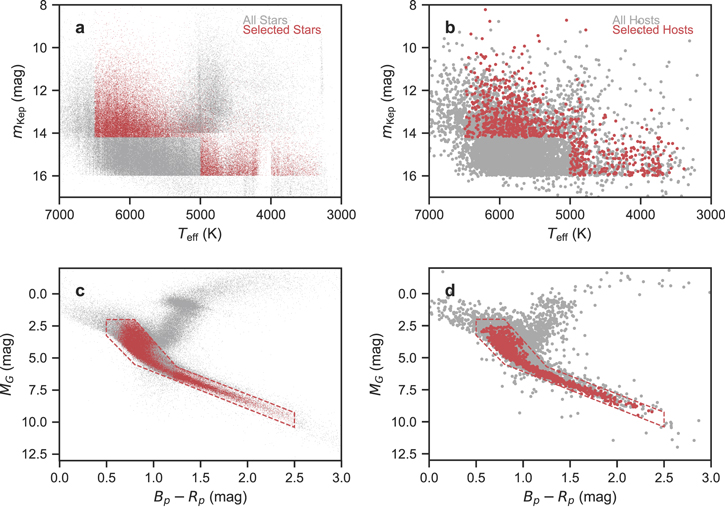
Figure 1. Panel (a): gray points show effective temperature and apparent magnitude mKep of stars observed by Kepler; red points are stars that pass the selection criteria described in Section 2. Panel (b): same as panel (a) but for planet hosts. Panel (c): same as panel (a) but showing Gaia absolute G-band magnitude MG and Bp − Rp color. The boundaries of our main-sequence filter are shown as red dashed lines. Panel (d): same as panel (c) but for planet hosts.
Download figure:
Standard image High-resolution imageWe began with 184,933 stars in the union of the following three catalogs: the Kepler project Data Release 25 (DR25) stellar properties catalog (Mathur et al. 2017, hereafter M17 ), the Gaia DR2 catalog (Gaia Collaboration et al. 2018), and the Berger et al. (2020b, hereafter B20) catalog of stellar properties. We then applied the following filters.
- 1.Stellar brightness and effective temperature. Our sample consists of two magnitude-limited components. If Teff = 5000–6500 K (as measured by M17), we required mKep < 14.2; if Teff = 3000–5000 K, we required mKep < 16.0. A total of 77,243 stars remained.
- 2.Main-sequence stars. We selected main-sequence stars using their position in the Gaia color–magnitude diagram. Stars were included if they reside within the boundaries shown in Figure 1. A total of 47,502 stars remained.
- 3.Single stars: Gaia source catalog. If a transit is observed within a Kepler aperture containing more than one star, it is often not possible to identify the star hosting the transiting object. Whichever star is the host, the transit depth is diluted by the neighboring star(s), and the inferred planet radius will be biased to smaller values. To ensure high-precision Rp , we worked to exclude targets that are diluted by >10%, which would result in an Rp error of >5%. We excluded stars where the cumulative G-band flux contribution from all Gaia-identified neighboring stars within 4″ exceeded 10%. Companions outside of this limit are resolved as separate sources in the KIC, which had an average FWHM of 2
5 (Brown et al. 2011). The Kepler project removed the diluting flux from such sources during the photometric extraction (see the discussion of the “crowding metric” in Stumpe et al. 2012). A total of 46,468 stars remained.
- 4.Single stars: Gaia astrometric noise. Companions within 1″ are often not resolved as separate sources in Gaia DR2 but can be identified using the residuals to the astrometric fits. The Gaia renormalized unit weight error (RUWE) is conceptually similar to the square root of the reduced χ2 and close to unity when the astrometric data are consistent with parallax and proper motion only, with no additional variation due to any companions (Lindegren 2018). Analyses of stars with high-resolution imaging have demonstrated that requiring RUWE < 1.2 removes companions with ΔmG < 3 mag and separations of ρ = 0
We cross-referenced these stars against the Thompson et al. (2018, hereafter T18) catalog of KOIs, which we accessed from the NASA Exoplanet Archive (NEA; Akeson et al. 2013). This catalog was derived from the final planet search conducted by the Kepler project (DR25). Among our filtered stellar sample, T18 lists 39,423 stars hosting 2373 KOIs. We subjected the KOIs to the following additional filters.
- 5.Candidate reliability. T18 dispositioned KOIs using a fully automated procedure called the Robovetter that performed a series of tests on a suite of data quality metrics designed to identify false positives due to data anomalies and eclipsing binaries. When setting the Robovetter thresholds, T18 emulated the human classification of the Threshold Crossing Event Review Team. Robovetter dispositioned all KOIs as either “false positive” or “planet candidate.” Some KOIs fall near the boundary between the two dispositions. Through Monte Carlo simulations, T18 quantified the proximity of each KOI to this boundary. They reported a “disposition score,” which is the fraction of Monte Carlo simulations classified as planet candidates. We required “planet candidate” status 13 with a disposition score 14 exceeding 75%. Finally, we removed a handful of known false positives that cleared the Robovetter that are listed in the DR25 supplemental table. 15 A total of 1425 KOIs orbiting 1003 host stars remained.
- 6.Candidate signal-to-noise ratio (S/N). Low-S/N candidates are more likely to be false positives (see, e.g., Bryson et al. 2020) and yield lower overall precision on Rp /R⋆. The Kepler project reported S/N as a “multiple event statistic” (MES; Jenkins 2002). 16 We required MES > 10. A total of 1250 KOIs orbiting 891 host stars remained.
- 7.Transit modeling. To compute planet properties, we used posterior samples of transit parameters derived from Markov Chain Monte Carlo (MCMC). A small fraction of the T18 KOIs were not modeled using MCMC. 17 Most of these are dispositioned as false positives. We removed a handful of candidates that passed the previous cuts. A total of 1246 KOIs orbiting 888 host stars remained.
Figure 1 shows the application of these filters to the field star and planet samples. In this paper, we refer to these 888 stars as the “CKS extended mass” (CXM) sample.
3. Spectroscopic Observations
We worked to compile a homogeneous spectroscopic catalog of all CXM stars from new and archival observations. All spectra were obtained with Keck/HIRES (Vogt et al. 1994) to ensure common systematics in our analysis. Our goal was to gather spectra with R ≥ 60,000 and S/N ≥ 20 pixel−1 on blaze at 5500 Å.
The inventory of DR1/DR2 spectra and the CXM host star sample are shown in Figure 2. By design, there was substantial overlap between the 1305-star DR1 sample and the CXM sample (628/888 spectra). The DR1 spectra have R ≥ 60,000 and S/N ≥ 45 pixel−1 and thus met our spectral quality goals. The 411 spectra in DR2 are a mixture of 81 archival HIRES spectra taken before 2018 and 330 new spectra taken by our team since then. For the archival spectra, all have R ≥ 60,000, and all but four had S/N ≥ 20 pixel−1. An additional 260/888 CXM stars have spectra in DR2.
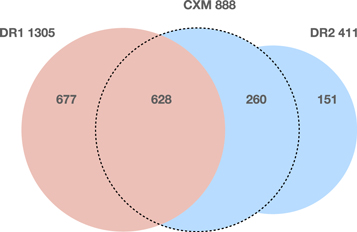
Figure 2. Venn diagram illustrating the number of host stars belonging to various samples described in this paper. CXM: 888 stars in the extended stellar-mass sample described in Section 2 that forms the basis of the exoplanet demographic work described in Sections 6 and 7. DR1: 1305 stars from Petigura et al. (2017). DR2: 411 stars with new spectra presented in this work.
Download figure:
Standard image High-resolution imageBelow, we describe the observations of the post-2018 DR2 spectra, which were executed as part of a NASA Key Strategic Mission Support program (PI: Petigura). Our strategy was identical to that of CKS DR1, except we exposed to a lower S/N. We used the standard setup of the California Planet Search (CPS; Howard et al. 2010). We observed stars through the “C2” slit with sky-projected dimensions of 086 × 14
0, which achieves a spectral resolution of R ≈ 60,000. We used the exposure meter to attain a designed S/N, which is measured at the peak of the blaze function at λ = 5500 Å.
Given the magnitude-limited nature of DR1, most DR2 stars had mKep = 14.2–16.0 mag. It would have been prohibitively expensive to observe these stars to the same S/N level as DR1 (45 pixel−1), so we used the exposure meter to achieve S/N = 20 pixel−1 for stars in this magnitude range. In Section 4, we demonstrate that the additional photon-limited uncertainties are smaller than other sources of uncertainty in the extracted parameters.
For faint targets, the sky background is occasionally comparable to the stellar spectrum, depending on moon separation, moon phase, and cloud cover. In our spectral reduction, we removed the sky background (see Batalha et al. 2011 for details), but it still contributes to exposure meter counts. Thus, at a fixed mV and exposure meter setting, additional sky background would cause exposures to terminate early. While at the telescope, we used a custom script to compute the sky contribution in real time and adjusted the exposure meter setting such that we would reach the desired S/N after sky subtraction.
We reduced our spectra according to the standard practices of CPS. We removed the blaze function by dividing our spectra by a composite spectrum of spectrally flat standards compiled by Clubb et al. (2018). One component of our spectroscopic analysis involved registering each spectrum to a common wavelength scale. We used the SpecMatch-Empirical code (Yee et al. 2017), which includes a ladder of reference spectra that have been registered against the National Solar Observatory solar atlas (Kurucz et al. 1984). Figure 3 shows the Mg i b region for representative spectra over a range of Teff. The deblazed spectra are available via the Keck Observatory Archive, 18 the CFOP website, 19 and a website maintained by our team. 20 We have also made available the standard observatory-frame wavelength solution applicable to every spectrum, which is accurate to within 1 reduced pixel or 1.2 km s−1. The registered spectra are also available at the above repositories.
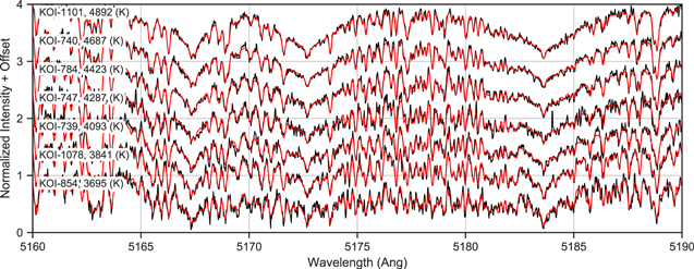
Figure 3. The black lines show a segment of HIRES spectra containing the Mg i b triplet for seven representative spectra observed by our team to illustrate the spectral resolution R ≥ 60,000 and S/N ≥ 20 pixel−1 (see Section 3). The red lines are SpecMatch-Empirical fits (see Section 4.1).
Download figure:
Standard image High-resolution image4. Host Star Characterization
4.1. Spectroscopy
We derived stellar parameters from our spectra using two related and complementary codes: SpecMatch-Synthetic and SpecMatch-Empirical. Both codes were designed to yield high-quality parameters even at moderate or low S/N. A detailed description of SpecMatch-Synthetic is available in Petigura (2015), and the code’s application to CKS DR1 is given in Petigura et al. (2017). In brief, the code generates a synthetic spectrum by interpolating within a set of library spectra computed over a grid of Teff,  , and [Fe/H]. It then applies line-broadening kernels that account for the instrumental profile, stellar rotation, and macroturbulence. The library spectra were computed by Coelho et al. (2005) under the assumption of local thermodynamic equilibrium (LTE) using the Castelli & Kurucz (2003) model atmospheres. The code derives Teff,
  , [Fe/H], and
  using nonlinear optimization of an l2 metric, which is evaluated over five spectral segments with a combined spectral bandwidth of 380 Å between 5200 and 6260 Å.
The uncertainties of the SpecMatch-Synthetic parameters have been extensively vetted for stars having Teff = 4700–6500 K. Errors are dominated by systematic uncertainties, which are σ(Teff) = 100 K,  dex, and σ([Fe/H]) =0.06 dex. Poisson uncertainties are smaller than systematic uncertainties even at low S/N because the code fits a wide spectral bandpass and combines information from many lines. At our lowest S/N (20 pixel−1), photon-limited errors are σ(Teff) = 34 K,
  dex, and σ([Fe/H]) =0.02 dex, respectively, below the systematic floor. Above 6500 K, the quality of the derived parameters degrades due to the reduced number of lines and substantial rotational broadening. As Teff drops below 4700 K, the number of lines in SpecMatch-Synthetic wavelength regions increases dramatically due to molecular features (of which MgH is the most prominent). The synthetic spectra do not accurately reproduce these complex spectra, and the derived parameters suffer.
By design, the CXM sample included many stars cooler than 4700 K, so we needed another method that is better suited to cool stars. In preparation for this project, Yee et al. (2017) developed SpecMatch-Empirical, which sidesteps the difficulties of cool star spectral synthesis. In brief, SpecMatch-Empirical compares a target spectrum to a spectral library of 404 stars with precise and accurate Teff, R⋆, and [Fe/H] measured through a combination of the following techniques: interferometry, asteroseismology, line-by-line LTE spectral synthesis, and spectrophotometry. The code identifies the top five matches based on an l2 metric. The target spectrum is then fit using a linear combination of these five spectra over a broad 1000 Å spectral region spanning 5000–6000 Å. The extracted parameters are a weighted average of the input parameters. For the representative spectra in Figure 3, we have overplotted the best-fit spectra.
Yee et al. (2017) validated the precision and accuracy of SpecMatch-Empirical across the H-R diagram and found that the quality of the derived parameters varies in this space due to the relative density of library spectra. For stars having Teff = 3500–5000 K and [Fe/H] between −0.5 and +0.5 dex, the code achieves uncertainties of σ(Teff) = 60 K and σ([Fe/H]) = 0.12 dex. Because this code analyzes 1000 Å of spectrum, it is robust to photon-limited uncertainties at low S/N. For our lowest-S/N spectra at 20 pixel−1, Poisson uncertainties amount to σ(Teff) = 6 K and σ([Fe/H]) = 0.004 dex and thus contribute negligibly to the overall error budget.
Table 1 lists our adopted stellar parameters for the 1716 star union of DR1 and DR2. Given the relative strengths and weaknesses of the two codes, we split our sample into two groups at Teff = 4800 K, as measured by SpecMatch-Empirical. We report SpecMatch-Synthetic parameters for the 1350 stars above this threshold and SpecMatch-Empirical for the 366 below.
Table 1. Stellar Properties
| KOI | mK | π | Teff | [Fe/H] |

| Prov | R⋆ | M⋆,iso | R⋆,iso | ρ⋆,iso | age⋆,iso | πspec | SB2 | CXM |
|---|---|---|---|---|---|---|---|---|---|---|---|---|---|---|
| (mag) | (mas) | (K) | (dex) | (km s−1) | (R⊙) | (M⊙) | (R⊙) | (g cc−1) | (Gyr) | (mas) | ||||
| 1 | 9.85 | 4.67 | 5857 | 0.02 | 1.3 | syn | 1.04 | 1.02 | 1.03 | 0.91 | 3.7 | 4.76 | 1 | 1 |
| 2 | 9.33 | 2.96 | 6403 | 0.22 | 5.1 | syn | 2.00 | 1.50 | 1.99 | 0.19 | 1.8 | 3.72 | 1 | 1 |
| 3 | 7.01 | 26.50 | 4619 | 0.16 | ⋯ | emp | 0.78 | 0.76 | 0.75 | 1.79 | 11.2 | 23.80 | 1 | 1 |
| 4 | 10.20 | 1.29 | 5948 | −0.27 | 38.0 | syn | 3.26 | 1.45 | 3.22 | 0.04 | 2.0 | 0.93 | 3 | 0 |
| 6 | 10.99 | 2.13 | 6356 | 0.05 | 11.8 | syn | 1.29 | 1.23 | 1.28 | 0.57 | 1.5 | 2.24 | 1 | 0 |
Note. Properties of 1716 planet-hosting stars from the union of the DR1 and DR2 data sets. Here mK
is the 2MASS K-band apparent magnitude, and π is the Gaia DR2 parallax. The Teff, [Fe/H], and  were derived by one of two methods listed in the “Prov” column: “syn,” SpecMatch-Synthetic, and “emp,” SpecMatch-Empirical. Here R⋆ is our adopted stellar radius from the Stefan–Boltzmann law. Stellar properties with the “iso” subscript incorporate constraints from the MIST isochrones. Here “SB2” encodes the limits on spectroscopic binaries (SB2s) using the ReaMatch code (Kolbl et al. 2015): 1, no detection of SB2 with ΔmV
≲ 5 mag and ΔRV ≳ 12 km s−1; 2, Teff < 3500 K, star unfit for ReaMatch; 3,
were derived by one of two methods listed in the “Prov” column: “syn,” SpecMatch-Synthetic, and “emp,” SpecMatch-Empirical. Here R⋆ is our adopted stellar radius from the Stefan–Boltzmann law. Stellar properties with the “iso” subscript incorporate constraints from the MIST isochrones. Here “SB2” encodes the limits on spectroscopic binaries (SB2s) using the ReaMatch code (Kolbl et al. 2015): 1, no detection of SB2 with ΔmV
≲ 5 mag and ΔRV ≳ 12 km s−1; 2, Teff < 3500 K, star unfit for ReaMatch; 3,  > 10 km s−1, star unfit for ReaMatch; 4, ambiguous detection; 5, obvious detection. Note: ReaMatch computes Teff and
  independently from SpecMatch-Synthetic and SpecMatch-Empirical. The “CXM” flag is 1 if the star is in the 888-star CXM subset. Median uncertainties are as follows: mK
, 0.02 mag; π, 1.4%; Teff, 100 K; [Fe/H], 0.06 dex;
independently from SpecMatch-Synthetic and SpecMatch-Empirical. The “CXM” flag is 1 if the star is in the 888-star CXM subset. Median uncertainties are as follows: mK
, 0.02 mag; π, 1.4%; Teff, 100 K; [Fe/H], 0.06 dex;  , 1 km s−1; R⋆, 3.9%; M⋆,iso, 3.7%; R⋆,iso, 2.6%; ρ⋆,iso, 8.9%; age⋆,iso, 0.24 dex; πspec, 16%.
Only a portion of this table is shown here to demonstrate its form and content. A machine-readable version of the full table is available.
Download table as: DataTypeset image
In the following section, we combine our spectroscopic Teff and [Fe/H] measurements with astrometric and photometric constraints to characterize the stellar hosts. Before proceeding, we note that the input spectra have a bimodal distribution of S/N and consider whether this could bias the DR1 and DR2 stellar parameters relative to one another. As explained above, the photon-limited Teff and [Fe/H] errors at S/N = 20 pixel−1 are less than half the systematic errors. Any S/N-dependent offsets are washed out by the larger systematic uncertainties.
4.2. Stellar Properties
We derived stellar masses, radii, and ages using our spectroscopic measurements of Teff and [Fe/H], along with astrometric and photometric constraints. Our methodology closely follows that of Fulton & Petigura (2018). We give a brief summary below, noting differences where relevant.
We measured R⋆ using the isoclassify package in its “direct” mode. This code evaluates R⋆ from the Stefan–Boltzmann law,

where Lbol is the bolometric stellar luminosity, and σsb is the Stefan–Boltzmann constant. Here Lbol is directly related to bolometric magnitude Mbol, which may be expressed as

where m is the apparent magnitude, μ is the distance modulus, A is the line-of-sight extinction, and BC is the bolometric correction. We summarize each input below, along with their typical uncertainties. Given the discontinuity in our sample selection at mKep = 14.2 described in Section 2, we report median uncertainties above and below this value.
- 1.Apparent magnitude. We used Two Micron All Sky Survey (2MASS) K-band photometric measurements because dust extinction is less severe in the infrared. We used 2MASS mK , which has a median precision of 0.02 mag for mKep < 14.2 and 0.03 mag for mKep > 14.2.
- 2.
- 3.Distance modulus. We used Gaia DR2 parallaxes and applied a correction of +0.053 mas to account for a known systematic offset in the Kepler field (Zinn et al. 2019). The parallaxes have a median precision of 1.2% for mKep < 14.2 and 1.8% for mKep > 14.2. Isoclassify handles the conversion between parallax and distance modulus using a Bayesian framework.
- 4.Bolometric correction. Isoclassify interpolates over a grid of bolometric corrections computed by the MESA Isochrones and Stellar Tracks project (MIST v1.2; Paxton et al. 2011, 2013, 2015; Choi et al. 2016; Dotter 2016). Uncertainties in Teff dominate the uncertainty of the K-band bolometric correction, and a 60 K uncertainty translates to an ≈0.03 mag error on BC.
Table 1 lists our measured R⋆, and Figure 4 shows the distribution of fractional R⋆ uncertainties. The median fractional uncertainty is 4.0% for mKep < 14.2 and 4.4% for mKep > 14.2.
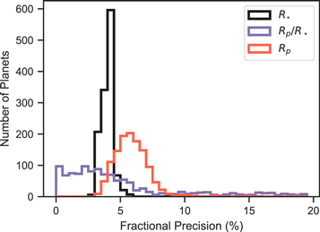
Figure 4. Fractional precision of Rp , R⋆, and Rp /R⋆ for the planets in the CXM sample.
Download figure:
Standard image High-resolution imageWe also ran isoclassify in its “grid” mode with the same constraints. In this mode, the code queries the MIST isochrones, which provide various stellar properties over a grid of M⋆, [Fe/H], and age. The grid extends to 20 Gyr to minimize grid edge effects, which can bias the parameter posteriors. At each grid point, isoclassify computes the likelihood that the point is consistent with the input constraints.
Marginalized values are determined by direct integration. We list M⋆,iso, R⋆,iso, ρ⋆,iso, and age⋆,iso in Table 1. The “iso” subscript indicates that these parameters are forced to be consistent with MIST isochrones. The median fractional uncertainty for M⋆,iso is 3.8% for mKep < 14.2 and 3.7% for mKep > 14.2; for ρ⋆,iso, it is 8.7% for mKep < 14.2 and 3.8% for mKep > 14.2. A handful of stars have age⋆,iso > 14 Gyr because the grid extends to 20 Gyr for the reasons explained above. Age uncertainties vary widely across the H-R diagram and are discussed in Section 6.
5. Planet Catalog
In the previous section, we computed stellar properties in the combined DR1/DR2 data set. For the remainder of the paper, we focus on the 1246 planets associated with the 888-star CXM subsample (see Figure 2). In this section, we first compute the planet properties given our updated stellar properties and then apply an additional set of quality checks to produce a high-reliability sample of planets for demographic work in later sections.
5.1. Planet Properties
We computed Rp from our R⋆ (listed in Table 1) and T18's modeling of Kepler light curves. We multiplied our posterior samples on R⋆ by the MCMC-derived posterior samples on Rp /R⋆ (available at the NEA). The median fractional error on Rp /R⋆ is 3.9% for mKep < 14.2 and 4.8% for mKep > 14.2. Uncertainties in R⋆ and Rp /R⋆ are independent and propagated into Rp , and we quote the 16th, 50th, and 84th posterior quantiles in Table 2. The median fractional precision in Rp is 5.6% for mKep < 14.2 and 6.3% for mKep > 14.2. Figure 4 shows the fractional precision of Rp , R⋆, and Rp /R⋆. For most of the sample, R⋆ errors are comparable to or larger than Rp /R⋆ errors. However, for a small subset, Rp /R⋆ errors dominate.
Table 2. Planet Properties
| Planet | P | Rp /R⋆ | T | Rp |

| a | Sinc | samp |
|---|---|---|---|---|---|---|---|---|
| (days) | (%) | (hr) | (R⊕) | (hr) | (au) | (S⊕) | ||
| K00001.01 | 2.5 | 12.39 | 1.29 | 14.04 | 2.83 | 0.037 | 814.85 | 0 |
| K00002.01 | 2.2 | 7.52 | 3.55 | 16.42 | 4.58 | 0.039 | 3855.68 | 1 |
| K00003.01 | 4.9 | 5.80 | 2.23 | 4.92 | 2.84 | 0.053 | 80.94 | 1 |
| K00007.01 | 3.2 | 2.45 | 3.84 | 4.07 | 4.29 | 0.046 | 1082.71 | 1 |
| K00010.01 | 3.5 | 9.21 | 2.75 | 15.51 | 4.47 | 0.050 | 1262.15 | 1 |
Note. Properties of 1246 planets orbiting the 888-star CXM sample. Orbital period P, planet-to-star radius ratio Rp
/R⋆, and transit duration T were measured from Kepler photometry by Thompson et al. (2018). Here Rp
follows from Rp
/R⋆ and R⋆. The expected duration of a centrally transiting object on a circular orbit  , semimajor axis a, and incident bolometric flux Sinc are determined from Kepler’s third law and the Stefan–Boltzmann law. The “samp” flag is 1 if the planet is in the curated sample of 970 planets described at the end of Section 5. Median uncertainties are as follows: P, 3 ppm; Rp
/R⋆, 4.3%; T, 2.3%, Rp
, 5.7%;
, semimajor axis a, and incident bolometric flux Sinc are determined from Kepler’s third law and the Stefan–Boltzmann law. The “samp” flag is 1 if the planet is in the curated sample of 970 planets described at the end of Section 5. Median uncertainties are as follows: P, 3 ppm; Rp
/R⋆, 4.3%; T, 2.3%, Rp
, 5.7%;  , 2.9%; a, 1.2%; Sinc, 9.2%.
Only a portion of this table is shown here to demonstrate its form and content. A machine-readable version of the full table is available.
Download table as: DataTypeset image
A note about the provenance of Rp /R⋆: there are a number of published catalogs of Rp /R⋆ from the Kepler project, of which T18 is the most recent. The NEA table corresponding to the T18 catalog lists the “best-fit” Rp /R⋆, not the posterior medians. Petigura (2020) found that these best-fit values contribute noise to Rp /R⋆ from the nonlinear optimization and recommended using posterior medians, which are a more robust estimator.
We compared our planet radii to T18 by computing the ratio of the radii, r = Rp,us/Rp,T18. There was a negligible systematic offset mean(r) = 1.00 but a substantial dispersion rms(r) = 20%. The dispersion is dominated by uncertainties in the T18 Rp .
Two additional quantities were relevant to our goal of precise planet radii: the observed transit duration T and the expected duration of a centrally transiting planet on a circular orbit  . Here T refers to the time between the midpoints of first/second contact and third/fourth contact. In the T18 modeling, the transit shape was set by the following free parameters: period P, transit epoch T0, impact parameter b, mean stellar density assuming a circular orbit ρ⋆,circ, and Rp
/R⋆. We derived T and its uncertainties according to
. Here T refers to the time between the midpoints of first/second contact and third/fourth contact. In the T18 modeling, the transit shape was set by the following free parameters: period P, transit epoch T0, impact parameter b, mean stellar density assuming a circular orbit ρ⋆,circ, and Rp
/R⋆. We derived T and its uncertainties according to

using the T18 MCMC chains. We computed  according to

Both T and  are listed in Table 2, along with semimajor axis a and incident stellar flux Sinc.
5.2. Refining the Planet Sample
While the initial CXM sample was optimized for high-reliability planets (Section 2), we incorporated additional diagnostics from our spectra to further increase sample purity. We first filtered on the following stellar properties.
- 1.
- 2.Spectroscopic parallax. Following Fulton & Petigura (2018), we used isoclassify to compute a “spectroscopic parallax” constrained by our Teff, [Fe/H], mK , and the MIST models. If the spectroscopic and trigonometric parallaxes differ significantly, we conclude that the input parameters used to compute R⋆ are inconsistent due to unresolved binaries or other effects. We removed nine stars where these parallaxes differed by 4σ or more. We chose a 4σ over a 3σ threshold because the probability of a 3σ event is 3 × 10⁻³; thus, we expect ≈three such events in a sample of ≈103 stars. The probability of a 4σ event is 6 × 10⁻⁵, so a single such event is unlikely. A total of 1215 KOIs orbiting 862 hosts remained.
- 3.Secondary spectra. We removed one star where we identified a secondary set of spectral lines using the methodology of Kolbl et al. (2015), which is sensitive to binaries having ΔmV ≲ 5 mag and Δv ≳ 12 km s−1. A total of 1214 KOIs orbiting 861 hosts remained.

Next, we filtered based on the following planet properties.
- 14.Impact parameter. We removed grazing and high impact parameter planets by excluding planets where the median of the b posterior exceeded 0.8. Petigura (2020) found, however, that for most Kepler light curves, this cut is ineffective at excluding high-b transits because b is nearly unconstrained. For such transits, Rp /R⋆ is biased by 10%–20% due to the strong b–Rp /R⋆ covariance. However, T/
 is an effective proxy for b. In addition to our explicit filter on b, we also required in order to exclude transits with b > 0.8. While planets with eccentric orbits that transit near periastron also produce low T/, Petigura (2020) showed that fewer than 20% of Kepler planets with have b < 0.8. A total of 973 KOIs orbiting 704 hosts remained.
 - 15.Radius precision. We required fractional errors on Rp of 20% or less. A total of 970 KOIs orbiting 703 hosts remained.


The properties of the stars that passed these cuts are shown in Figure 5. They span a mass range of M⋆ ≈ 0.5–1.4 M⊙.
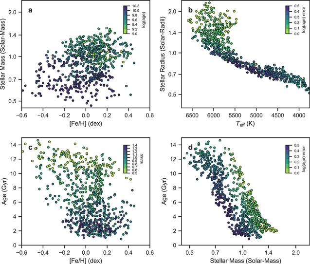
Figure 5. Properties of host stars in the filtered CXM sample described in Section 5.2. Panel (a): stellar mass and metallicity. Panel (b): stellar radius and effective temperature. The color scale conveys the isochrone age uncertainty in dex (half the difference between the 84th and 16th percentiles of the age posterior). Panel (c): stellar metallicity and age. Panel (d): stellar mass and age where the color scale is equivalent to panel (b). Several stars have ages exceeding 14 Gyr for reasons we explain in Section 4.2. We discuss correlations between mass, metallicity, and age in Section 6.2.
Download figure:
Standard image High-resolution image6. Distribution of Detected Planets
From here on, we describe and interpret the features in our curated sample of 970 planets. In this section, we treat the population of detected planets before turning to the occurrence distribution in Section 7. We explore how the radius gap correlates with P, Sinc, M⋆, and age in Section 6.1. We then inspect how the super-Earth and sub-Neptune populations vary with stellar mass in Section 6.2.
6.1. Dependence of the Radius Gap on Period, Flux, Stellar Mass, and Stellar Metallicity
Figure 6 shows several views of our planet sample. The y-axes show updated Rp , and the x-axes show P, Sinc, M⋆, and [Fe/H]. The contours show the relative density of detected planets in these domains using a Gaussian kernel density estimation (KDE), and the KDE bandwidths are specified in the caption. Figure 7 is analogous to Figure 6 but with Rp restricted to 1–4 R⊕ for a detailed view of the radius gap.
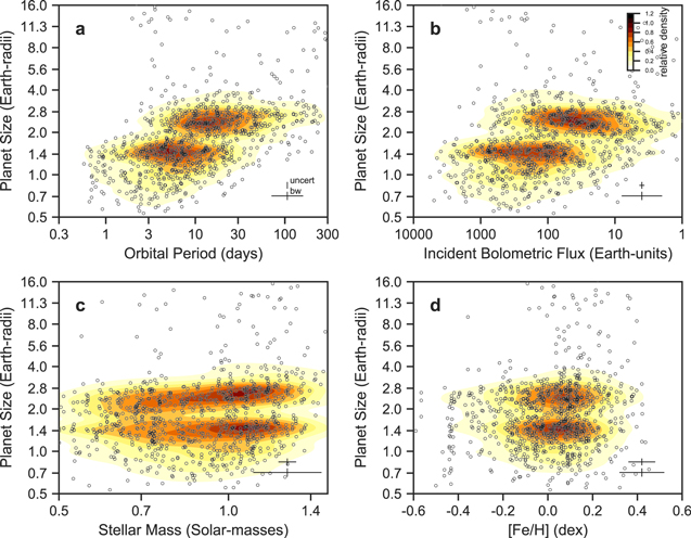
Figure 6. Panel (a): sizes and orbital periods of detected planets after applying the filters described in Section 5.2. The contours show a Gaussian kernel density estimate (KDE) of the number density of planets in this space. The kernel bandwidth is 0.029 dex in Rp and 0.18 dex in P, as shown by the symbol labeled “bw.” The “uncert” symbol shows the median Rp uncertainty (P uncertainties are smaller than the line width). Panels (b)–(d): same as panel (a), except that the x-axis is Sinc, M⋆, and [Fe/H], and the kernel bandwidths along the horizontal axes are 0.30, 0.061, and 0.1.
Download figure:
Standard image High-resolution image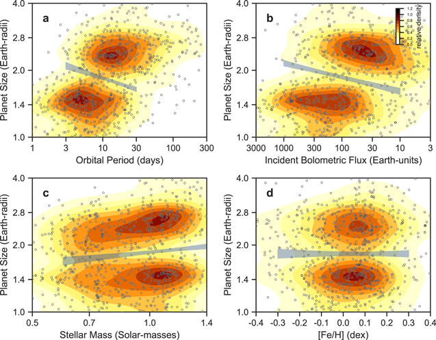
Figure 7. Zoomed-in version of Figure 6 highlighting the radius gap, which is visible in all projections. In the M⋆ projection, the typical sub-Neptune becomes larger with M⋆, while the super-Earths remain the same size. The bands are power-law fits of the radius gap (see Section 6.1).
Download figure:
Standard image High-resolution imageThe P–Rp distribution and closely related Sinc–Rp distribution of Kepler planets have been extensively studied in previous works. We begin by remarking on several known features that appear in our extended stellar-mass sample. Most Kepler planets fall into one of two size categories: super-Earths and sub-Neptunes. For definitiveness, we adopt the following size limits for the two planet classes: Rp = 1.0–1.7 and 1.7–4.0 R⊕. The radius gap separating the populations was observed by Fulton et al. (2017) in CKS DR1 (M⋆ ≈ 0.8–1.3 M⊙), Van Eylen et al. (2018) in a sample of stars with asteroseismic detections (M⋆ ≈ 1.0–1.4 M⊙), and other subsequent works. We again resolve the radius gap, despite the broader M⋆ range of the CXM sample (M⋆ ≈ 0.5–1.4 M⊙).
The distribution of super-Earths is centered at shorter periods and higher incident fluxes than the distribution of sub-Neptunes. Compared to super-Earths, there are few sub-Neptunes with P < 3 days or Sinc > 300 S⊕. This paucity of sub-Neptunes is not a selection effect because larger planets are easier to detect. This zone of low sub-Neptune occurrence is sometimes referred to as the sub-Neptune desert (see, e.g., Szabó & Kiss 2011; Beaugé & Nesvorný 2013; Lundkvist et al.2016). In Section 7, we quantify the sharpness of this boundary and explore its dependence on stellar mass. The relative lack of super-Earths at P > 30 days and Sinc < 10 S⊕ is closely tied to survey completeness, also addressed in Section 7.
We wish to characterize the slope of the radius gap in P–Rp and Sinc–Rp space because it is a metric by which to test theoretical predictions. However, fitting a parameterized description of the radius gap is challenging, since it involves characterizing the absence of planets. Van Eylen et al. (2018) used a support vector classification (SVC) scheme to find the line that maximized the distance between the super-Earth and sub-Neptune populations. The SVC scheme struggles for our sample because the gap is not devoid of planets. (Recently, David et al. 2021 investigated how regularization can assist the SVC identification of the radius gap in the CKS sample.)
We adopted a different approach, starting with the relative number density of detected planets in the P–Rp
plane  as measured by our KDE. This quantity is shown as contours in Figure 7(a). We then found the minimum density along 100 vertical lines spanning
  = 0.15–0.35 spaced uniformly in
  over 0.5–1.5. We then fit the train of 100 minima with following power law:

where the slope m and intercept Rp,0 are free parameters. To be clear, Rp,0 should be interpreted as the midpoint of the radius gap at 10 day orbital periods. We chose 10 days as a convenient reference point near the middle of the super-Earth and sub-Neptune populations shown in Figure 7(a). To determine uncertainties, we generated 1000 bootstrap resamples with replacement of the planet population shown in Figure 7(a) (Press 2002). For each bootstrapped population, we recomputed the planet number density with our KDE, the train of minima, and the best-fitting power law. We found  and Rp,0 =
  R⊕, which reflect the 16th, 50th, and 84th percentiles. Figure 7 shows the credible gap models. We explored the sensitivity of our method to different period ranges by perturbing the upper and lower boundaries by ±0.25 dex. The derived parameters were consistent to 1σ. We also explored the sensitivity of our method to our adopted KDE period bandwidth. A very wide bandwidth will flatten the radius gap (i.e., bias ∣m∣ toward smaller values). We repeated our analysis with a much smaller bandwidth of 0.04 dex and found that m and Rp,0 changed by less than 1σ.
We performed similar analyses to fit the radius gap as a function of Sinc, M⋆, and [Fe/H]. Table 3 lists the parametric models used in the fits and the credible range of parameters. Figure 7 shows the range of credible gap models. We observed a positive slope with incident flux ( ), a positive slope with stellar mass (
 ), and no significant correlation with metallicity (
![$d\mathrm{log}{R}_{p}/d[\mathrm{Fe}/{\rm{H}}]\,={0.01}_{-0.06}^{+0.05}$](https://content.cld.iop.org/journals/1538-3881/163/4/179/revision1/ajac51e3ieqn31.gif) ).
).
Table 3. Power-law Fits to the Radius Gap
| Fit | M⋆ | m | Rp,0 | Dist. |
|---|---|---|---|---|
Rp
= Rp,0

| 0.5–1.4 |

|

| D |
| 0.5–0.7 |

|

| D | |
| 0.7–1.0 |

|

| D | |
| 1.0–1.4 |

|

| D | |
| 0.5–0.7 |

|

| O | |
| 0.7–1.0 |

|

| O | |
| 1.0–1.4 |

|

| O | |
Rp
= Rp,0

| 0.5–1.4 |

|

| D |
| 0.5–0.7 |

|

| D | |
| 0.7–1.0 |

|

| D | |
| 1.0–1.4 |

|

| D | |
| 0.5–0.7 |

|

| O | |
| 0.7–1.0 |

|

| O | |
| 1.0–1.4 |

|

| O | |
Rp
= Rp,0

| 0.5–1.4 |

|

| D |
| Rp = m [Fe/H] + Rp,0 | 0.5–1.4 |

|

| D |
Note. We fit the radius gap in the detected planet population in Section 6.1 as a function of orbital period, incident stellar flux, stellar mass, and stellar metallicity (see Figure 7). We repeated the orbital period and incident flux fits for narrower ranges of stellar mass (see Figures 8 and 9). We fit the radius gap in the debiased planet occurrence distribution in Section 7.1 (see Figures 8 and 9). We elaborate on the following columns: “Fit” is the functional form of the fit, “M⋆” is the range of stellar masses, and “Dist.” indicates whether the fit was of the distribution of planet detections “D” or occurrence “O.”
Download table as: ASCIITypeset image
We explored how the P–Rp distribution of planets changes with M⋆. The left panels of Figure 8 shows this distribution for three different bins of stellar mass with the following boundaries: 0.5, 0.7, 1.0, and 1.4 M⊙. The super-Earth and sub-Neptune populations are distinct in each bin, but their locations vary with M⋆. As M⋆ increases, the population of super-Earths and sub-Neptunes separates; the super-Earth population is confined to Rp < 1.7 R⊕ while the sub-Neptunes grow in size. We measured the slope and intercept of the radius gap in these three bins. They are given in Table 3 and consistent to 2σ.
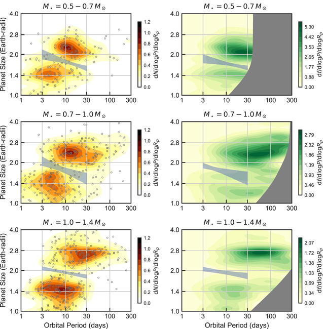
Figure 8. The left panels are analogous to Figure 7(a), except we have split the planet sample into three bins of stellar mass. The right panels show the ORD of planets  . The maximum ORD increases with decreasing M⋆ (note different color scales). Regions of low planet detectability, defined as ntrial < 50, are gray. The typical sub-Neptune size grows with M⋆, while super-Earths have a nearly constant size. The bands show fits to the radius gap.
Download figure:
Standard image High-resolution imageWe also explored how the Sinc–Rp distribution changes with M⋆. Figure 9 is analogous to Figure 8, except it shows the Sinc–Rp distribution for three bins of stellar mass. The credible models describing the radius gap in this space are consistent to 2σ.
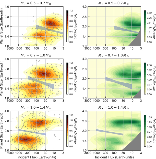
Figure 9. Same as Figure 8, except the x-axis is incident bolometric flux.
Download figure:
Standard image High-resolution image6.2. Dependence of Planet Size on Stellar Mass
In the previous section, we measured the slope of the radius gap in the Rp –M⋆ plane and noted that it increases with M⋆. Inspecting Figure 7(c), we see qualitatively that the radius gap trend is driven by the fact that the typical sub-Neptune grows with stellar mass, while the typical super-Earth does not. Here we quantify these trends and explore possible confounding factors.
We first measured the sub-Neptune Rp –M⋆ correlation by selecting all sub-Neptunes from the population shown in Figure 7 based on their radii (Rp = 1.7–4.0 R⊕). We then fit a power law,

We used the Levenberg–Marquardt algorithm as implemented in the lmfit Python package to find the best-fit parameters and measured uncertainties via 1000 bootstrap resamples. We detected a positive correlation between M⋆ and sub-Neptune size at 8σ significance, α = 0.25 ± 0.03. An identical analysis for the super-Earths (Rp = 1.0–1.7 R⊕) revealed no correlation, α = 0.02 ± 0.03.
Before interpreting these trends with M⋆, we must consider the confounding effects of other stellar properties that are correlated with M⋆. (We consider effects from the M⋆-dependent survey completeness in Section 7.2.) Stellar metallicity and age are both concerns because they are astrophysically correlated with mass. This M⋆–[Fe/H]–age correlation is tied to the chemical enrichment of the galaxy and stellar life spans. A star’s main-sequence lifetime is a strong function of its mass:  . Massive stars are younger, on average, and formed when the galaxy was more enriched in metals, as shown in Figures 5(a) and (c). Figure 5(b) highlights the variable uncertainties of our age measurements, which range from ≈0.1 dex for stars that have evolved off the main sequence to ≈0.5 dex for stars with Teff ≲ 5500 K, i.e., indistinguishable from the zero-age main sequence.
We quantified possible metallicity and age effects by including them in our regression:

When we allowed α and β to vary and fixed γ to zero, we found β = −0.01 ± 0.02 and –0.00 ± 0.02 for sub-Neptunes and super-Earths, i.e., no significant Rp –[Fe/H] correlation. Finally, we considered the effects of age by allowing γ to vary as well. We restricted our analysis to stars with Teff > 5500 K where age⋆,iso is not prior-dominated. We found γ = −0.01 ± 0.03 and 0.02 ± 0.02 for the sub-Neptunes and super-Earths, i.e., no Rp –age correlation.
Based on these fits, we concluded that stellar mass rather than metallicity or age is the property most closely linked to sub-Neptune size variation. We acknowledge two additional caveats to the above analysis, which we address in later sections. First, we fit the population of detected planets, which includes survey completeness effects that are addressed in Section 7.2. Second, orbital period is another possible confounding variable if the shape of the period distribution varies with stellar mass. Fortunately, as we show in Section 7.3, the period distribution is nearly independent of stellar mass up to a normalization constant.
7. Debiased Distribution of Planets
We have characterized the location and slope of the radius gap and its dependence on stellar mass. However, one must exercise caution when connecting these trends to planet formation models because the distributions of planets have been filtered through Kepler’s selection function. In this section, we remove selection effects to characterize variation in the planet population with stellar mass.
In Section 7.1, we reexamine the slope of the radius gap as a function of period and incident flux (first treated in Section 6.2) and find consistent results after accounting for selection effects. In Section 7.2, we measure the sizes of super-Earths and sub-Neptunes (as in Section 6.2) and observe the same qualitative trends after removing selection effects. In Section 7.3, we characterize how the period and incident flux distributions of super-Earths and sub-Neptunes vary with stellar mass.
7.1. Dependence of the Radius Gap on Stellar Mass
We return to the P–Rp
distribution of planets shown in Figure 8. We wish to remove Kepler’s observational biases to measure the planet occurrence rate density (ORD),  . One may integrate the ORD over a specified domain in the P–Rp
plane to derive the number of planets per star residing in that domain.
. One may integrate the ORD over a specified domain in the P–Rp
plane to derive the number of planets per star residing in that domain.
For every detected planet in a sample of n⋆ stars, a large number are missed due to nontransiting geometries or insufficient photometric S/N. We account for both effects here using the inverse detection efficiency method (IDEM; see Fulton & Petigura 2018). Each detected planet i with (P, Rp
) represents  total planets, where
  is the product of transit and detection probability averaged over the parent stellar population. We computed
  over a grid of (P, Rp
). The probability that a randomly inclined planet with semimajor axis a will transit with b < 0.8 is
over a grid of (P, Rp
). The probability that a randomly inclined planet with semimajor axis a will transit with b < 0.8 is  , assuming circular orbits. We computed
  for each star using the B20
R⋆ and deriving a from P and the B20
M⋆ using Kepler’s third law.
for each star using the B20
R⋆ and deriving a from P and the B20
M⋆ using Kepler’s third law.
We characterized the recovery rate  following the procedure described in Christiansen et al. (2020). These authors injected a suite of 146,295 synthetic transits into the raw Kepler pixel-level data and searched for transits using the same pipeline used to produce the T18 catalog. The output was a list of injections that were either successfully recovered or not. This list may be used to determine the average recovery rate for any Kepler sample of interest. We selected the subset of injections with P = 1–300 days into our parent stellar population described in Section 2 and measured the recovery rate as a function of the expected MES, a close relative of transit S/N. We modeled the completeness curve as a Γ cumulative distribution function:

The best-fit model had the coefficients (a, b, c) = (26.1, 0.320, 0.941) and is shown in Figure 10. We set the recovery rate to zero when MES < 10 to incorporate our filter described in Section 2. We evaluated the MES for each star based on the putative planet’s transit depth and duration and the star’s tabulated photometric noise (combined differential photometric precision; Jenkins et al. 2010).
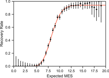
Figure 10. Points show the recovery rate of the Kepler planet detection pipeline of simulated planets injected by Christiansen et al. (2020) as a function of MES. The curve shows the parametric model we used to account for pipeline incompleteness in our occurrence calculations described in Section 7.
Download figure:
Standard image High-resolution imageWith our calculated weights w, we may now compute the total number of planets within a given region of the P–Rp plane by summing the weights of the planets within that region, ∑i wi , or compute the occurrence rate (number of planets per star) via (1/n⋆)∑i wi .
The IDEM, while mathematically straightforward, has some drawbacks, particularly when  is small. In brief, Hsu et al. (2018) showed that the IDEM is a biased estimator at low
  because the weights wi
are computed assuming no uncertainties in Rp
. Hsu et al. (2018) proposed a less biased estimator using approximate Bayesian computation (ABC). We avoided these complications by restricting our analysis to regions where
because the weights wi
are computed assuming no uncertainties in Rp
. Hsu et al. (2018) proposed a less biased estimator using approximate Bayesian computation (ABC). We avoided these complications by restricting our analysis to regions where  > 25%, where differences between the IDEM and ABC amount to <1σ (Fulton & Petigura 2018).
We measured the ORD in the three bins of stellar mass introduced in Section 6.2 via

where k is a 2D Gaussian with a bandwidth of  dex in P and
  = 0.02 dex in Rp
. The results are shown in the right panels of Figure 8. The value at each (P, Rp
) is the number of planets per star in a 1 dex × 1 dex interval centered at (P, Rp
). It is convenient to scale this value to smaller intervals because the ORD varies significantly over 1 dex in P and Rp
. For example, to read off the number of planets per star within a box having the dimensions of the kernel FWHM, multiply the ORD by 2.355 × 0.3 × 2.355 × 0.02 = 0.033.
= 0.02 dex in Rp
. The results are shown in the right panels of Figure 8. The value at each (P, Rp
) is the number of planets per star in a 1 dex × 1 dex interval centered at (P, Rp
). It is convenient to scale this value to smaller intervals because the ORD varies significantly over 1 dex in P and Rp
. For example, to read off the number of planets per star within a box having the dimensions of the kernel FWHM, multiply the ORD by 2.355 × 0.3 × 2.355 × 0.02 = 0.033.
We do not plot occurrence in regions of low planet detectability, defined to be where  . The ORD ranges from ≈zero to 4, which corresponds to ≈0–0.1 planets star–1 within the kernel FWHM. For (P, Rp
) values where
. The ORD ranges from ≈zero to 4, which corresponds to ≈0–0.1 planets star–1 within the kernel FWHM. For (P, Rp
) values where  , there are effectively 50 stars where such a planet could be detected, and we would expect zero to five detected planets within the kernel FWHM. At this point, Poisson fluctuations become unmanageable.
We fit a power law to the radius gap for each mass bin. Our methodology, power-law parameterization, fitting domain, and uncertainty analysis are identical to those presented in Section 6, except that we fit ORD rather than the density of the detected planets. The credible range of values is given in Table 3. The measured slope and intercepts are consistent at 1σ to those measured using planet detections only.
7.2. Dependence of Planet Size on Stellar Mass
In Section 6.2, we noted a positive Rp –M⋆ correlation for sub-Neptunes that was not mirrored by super-Earths. However, we must consider the possibility that such correlations (or lack thereof) could stem from the Kepler selection function. To do so, we first divided the CXM planet hosts and parent stellar population into our three M⋆ bins from Section 6.2. In order to treat hosts and nonhosts equally, we used the B20 M⋆, which is available for all stars.
Returning to our binned planet population, we computed the occurrence-weighted mean planet sizes for sub-Neptunes having P < 100 days and display them in Figure 11. Fitting the power law given by Equation (6) to the three binned mean size measurements shown in Figure 11 yields an index α = 0.23 ± 0.04 and an intercept of Rp,0 = 2.47 ± 0.03 R⊕ (uncertainties from bootstrap resampling). These values are consistent with our fits to the population of detected planets (Section 6.2). For the sub-Neptunes, the weights w are dominated by geometrical corrections that are independent of Rp . Planets with larger P have larger w and are more strongly weighted than in Section 6.2. However, given the lack of a significant tilt in the P–Rp distribution, the average value is similar.
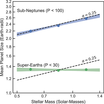
Figure 11. Mean size of super-Earths with P < 30 days and sub-Neptunes with P < 100 days. Over M⋆ = 0.5–1.4 M⊙, the average sub-Neptune grows from 2.1 to 2.6 R⊕ with a slope of  = 0.23 ± 0.04. The mean super-Earth has a nearly constant size of 1.35 R⊕ with α = −0.01 ± 0.03. Wu (2019) reported α = 0.25 for both populations and is shown by the dashed lines. Our sub-Neptune results are consistent with this index, but our super-Earth results are inconsistent at 8σ.
Download figure:
Standard image High-resolution imageCorrections stemming from low detectability are larger for the super-Earths. While there is no obvious tilt of the super-Earth population in Figure 7(c), completeness effects could conspire to produce a flat dependence when there is actually a positive slope in the underlying population. We computed the occurrence-weighted mean planet size for super-Earths with P < 30 days and found α = −0.01 ± 0.03 and Rp,0 = 1.34 ±0.01, i.e., no significant correlation. We interpret the different Rp –M⋆ correlation super-Earths and sub-Neptunes and compare our results to previous literature measurements in Section 8.
7.3. Orbital Period and Incident Flux Distributions
One key feature of the exoplanet population is the paucity of sub-Neptunes with P ≲ 10 days, i.e., the “sub-Neptune desert.” The edge of this desert is significant in both the core- and XUV-powered models. It represents a boundary, inside of which core-dominated planets (i.e., Mc ≫ Menv) cannot retain H/He envelopes and are completely stripped.
Here we characterize the edge of the sub-Neptune desert in terms of period and flux and note how it changes with stellar mass. One can see qualitatively from Figures 8 and 9 that the edge of the sub-Neptune desert occurs at a similar P for all mass bins but varies in Sinc by ∼10×. We first considered the edge in period space in our three bins of stellar mass introduced in Section 6.2. Quantitatively measuring this boundary in P by visually inspecting Figure 8 is suboptimal for a number of reasons. First, the contours do not convey uncertainties. Second, the Gaussian KDE used to generate the 2D distributions smears out sharp features in the P distributions. Third, the sub-Neptune desert is the paucity of short-period sub-Neptunes relative to long-period sub-Neptunes, but the contours show absolute occurrence, which also varies with stellar mass. These shortcomings motivated a different method, which we describe below.
Within each M⋆ bin, we modeled the ORD as

over a rectangular domain of P and Rp . Here f⋆ is the mean number of planets per star within the P–Rp domain. In principle, λ may be any function that integrates to unity over the same domain. We consider parametric functions described by a vector of parameters θ that we will constrain through Bayesian inference. In short, the free parameters f⋆ and θ control the normalization and shape of the ORD, respectively.
Following previous works, we modeled the detected population of planets as a realization of an inhomogeneous Poisson point process (see, e.g., Rogers & Owen 2021, and references therein). The log-likelihood of observing the full sample is given by

where

is the expected number of detected planets given f⋆ and
θ
. Here  .
.
For simplicity, we assumed that the period and radius distributions are independent, i.e., λ(P, Rp ) ∝ λ(P)λ(Rp ). We also approximated the Rp distribution log-uniform within the Rp boundaries, i.e., λ(Rp ) ∝ 1/Rp . We precomputed

to reduce Λ to a 1D integral,

Following Rogers & Owen (2021), we described the period distribution with a smooth broken power law,

where C is the constant of proportionality that enforces normalization. 21 In this parameterized description, P0 is the knee of the distribution; for P ≪ P0, the distribution approaches a power law with an index of k1, and for P ≫ P0, the index is k2.
We first fit the sub-Neptune distribution for our three bins of stellar mass over P = 1–300 days. Our goal was to characterize the knee and slope of the occurrence period distribution. For consistency between the subsamples, we fixed k2 = −1, i.e., log-uniform occurrence for P ≫ P0. We maximized the likelihood (Equation (11)) using the L-BFGS-B algorithm and explored the credible range of parameters using the MCMC sampler of Goodman & Weare (2010). We imposed log-uniform priors on f⋆ and P0 and a linear prior on k1. We sampled the posterior with eight walkers for 5000 steps each and discarded the first 1000 as burn-in. The chains for all parameters were at least 50 times longer than the integrated autocorrelation time, indicating convergence. Table 4 lists the 16th, 50th, and 84th percentiles of our posterior samples. Figure 12 shows the posterior probability density of f⋆ and P0 for different M⋆ bins.
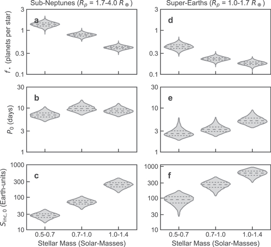
Figure 12. Panel (a): posterior probability density of the mean number of sub-Neptunes per star f⋆ with P = 1–300 days for three stellar-mass bins. Dashed lines show the 25%, 50%, and 75% quartiles. Panel (b) shows the period breakpoint P0. Panel (c) shows the flux breakpoint Sinc,0. Panels (d)–(f) are the same as panels (a)–(c) but for super-Earths. The mean occurrence in panel (d) corresponds to P = 1–30 days. For both classes of planets, there is a decline in total occurrence with increasing M⋆. For the sub-Neptunes, P0 ranges from ≈7.0 to 9.6 days, consistent to 40%; for the super-Earths, P0 is ≈2.7–5.1 days, consistent to a factor of 2. For the sub-Neptunes, the breakpoint Sinc,0 increases by a factor of 9 from  to
to  S⊕ between the low- and high-mass bin. For the super-Earths, the breakpoint also increases with stellar mass from
  to
to  S⊕, a factor of 7 increase.
Download figure:
Standard image High-resolution imageTable 4. Fits to the Planet Period and Flux Distributions
| Period | Flux | ||||||
|---|---|---|---|---|---|---|---|
| Size | M⋆ | f⋆ | P0 | k1 | f⋆ | Sinc,0 | k2 |
| SE | 0.5–0.7 |

|

|

|

|

|

|
| 0.7–1.0 |

|

|

|

|

|

| |
| 1.0–1.4 |

|

|

|

|

|

| |
| SN | 0.5–0.7 |

|

|

|

|

|

|
| 0.7–1.0 |

|

|

|

|

|

| |
| 1.0–1.4 |

|

|

|

|

|

| |
Note. In Section 7.3, we modeled both the period and flux distribution of super-Earths (SE) and sub-Neptunes (SN) for different bins of stellar mass. We used a smooth broken power law to model the period distribution  . Here f⋆ is the mean number of planets per star over the following period ranges: P = 1–30 days (SE) and P = 1–300 days (SN). The power-law indices below and above the breakpoint P0 are k1 and k2, respectively. In our modeling, k2 is fixed to −1, i.e.,
  constant for P ≫ P0. Similarly, we also used a smooth broken power law to model the flux distribution. Here k1 was fixed to −1.
Download table as: ASCIITypeset image
Figure 13 shows the best-fit and credible range of models for our three M⋆ bins. They are similar except for an overall shift in the normalization. For the low-, medium-, and high-mass bins, the breakpoint P0 is at  ,
,  , and
, and  days, respectively, consistent to 2σ. The power-law indices k1 agree to 1σ and are
  ,
,  , and
, and  we observed a steady decrease in the absolute number of planets per star from 0.5 to 1.4 M⊙ of
  , to
, to  , to
, to  .
.
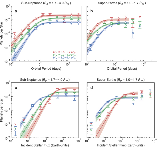
Figure 13. Panel (a): period distribution of sub-Neptunes for three bins of stellar mass. The points show the number of planets per star in period bins that are 0.25 dex wide. We modeled the ORD df/dP as a smooth broken power law, which we fit to the unbinned planet population over P = 1–300 days (see Section 7.3). The bands show the credible range of  dex. The height of each curve at a particular P is the number of planets per star within a 0.25 dex period interval centered at P. Panel (b): same as panel (a) except for super-Earths where the fits extend to 30 days. Panels (c) and (d): same as panels (a) and (b) except showing incident flux distribution. The vertical axis has the following interpretation: number of planets per star within a 0.5 dex flux interval.
Download figure:
Standard image High-resolution imageThe similarity of P0 for the different mass bins is noteworthy because it indicates a key boundary in the planet formation process that is stationary over a wide range of stellar mass. Naturally, a stationary P0 implies a variable Sinc,0 given the relationship between M⋆ and bolometric luminosity. To quantify this boundary in flux space, we again characterized the distribution as a smooth broken power law,

but fixed k1 to −1. Over the three M⋆ bins, we observed a factor of 9 increase in the breakpoint Sinc,0 from  , to
, to  , to
, to  S⊕.
S⊕.
We also characterized the period distribution of super-Earths. Our modeling was identical to that of the sub-Neptunes, except we only included planets out to 30 days due to low completeness at longer orbital periods. Here the breakpoint P0 increases with M⋆ from  , to
, to  , to
, to  days. The breakpoints in flux Sinc,0 occur at
  ,
,  , and
, and  S⊕. Figure 14 contrasts the super-Earth and sub-Neptune breakpoints. The super-Earth breakpoint is shifted to smaller orbital periods and higher incident fluxes for all stellar-mass bins. We interpret these shifts in Section 8.5.
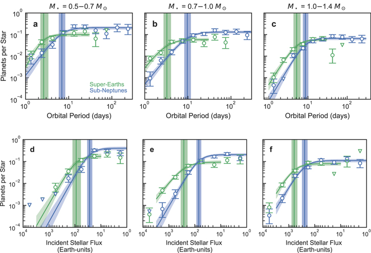
Figure 14. Panels (a)–(c): period distribution of super-Earths (green) and sub-Neptunes (blue) for different bins of stellar mass. Points and curves are the same as shown in Figure 13 but grouped according to stellar mass as opposed to planet size. The vertical bands show the range of credible period breakpoints P0. For all stellar-mass bins, P0 is smaller for super-Earths than for sub-Neptunes. Panels (d)–(f): same as panels (a)–(c), but the x-axis is incident stellar flux. The flux breakpoint Sinc,0 increases with stellar mass, but the relative offset between the two populations is nearly constant.
Download figure:
Standard image High-resolution image8. Discussion
8.1. Positive M⋆–Rp Correlation Suggests Massive Stars Make Massive Planet Cores
One of the striking features of Figure 7(c) is the divergence of the super-Earth and sub-Neptune populations with stellar mass; the sub-Neptunes grow larger, while the super-Earths do not. When we modeled the size dependence of each population as a power law,  , we found α = 0.25 ± 0.03 and 0.02 ± 0.03, respectively. The slope of the radius gap in M⋆–Rp
space (displayed in Figure 7) lies between those two values,
, we found α = 0.25 ± 0.03 and 0.02 ± 0.03, respectively. The slope of the radius gap in M⋆–Rp
space (displayed in Figure 7) lies between those two values,  .
.
A positive sub-Neptune Rp –M⋆ correlation has been noted in several previous works. Fulton & Petigura (2018) observed such a trend over a narrower stellar-mass range of ≈0.8–1.3 M⊙. Later, Wu (2019) stitched together the Fulton & Petigura (2018) sample with a compilation of ∼100 Kepler and K2 planets with hosts of M⋆ ≲ 0.7 M⊙ from Newton et al. (2015) and Dressing et al. (2017) and reported α = 0.23–0.35, consistent with what we found.
In contrast to the sub-Neptunes, we observe a flat super-Earth Rp –M⋆ dependence, α = −0.01 ± 0.03. This result differs from that of Wu (2019), who reported α = 0.23–0.35. As a point of comparison, Figure 11 shows our occurrence-weighted mean super-Earth size with an α = 0.25 dependence overplotted; such a strong relationship is ruled out at 8σ significance. The differences between the two works may stem from the fact that Wu (2019) used an admixture of planet samples with heterogeneously derived properties.
Berger et al. (2020a) offered a second point of comparison. They derived properties of 2956 KOIs spanning M⋆ ≈ 0.6–1.4 M⊙ that host 3898 confirmed/candidate planets. They measured the radius gap slope in M⋆–Rp
space and found  , which is consistent with our measured value, albeit with larger uncertainties.
What causes the super-Earth size to be independent of stellar mass while the sub-Neptune size grows with stellar mass? In our discussion below, we assume that planets between 1 and 4 R⊕ are Earth-composition bodies that may also include an H/He envelope. This assumption is supported by the growing body of mass measurements of planets in this size range (see, e.g., Weiss & Marcy 2014; Sinukoff 2018). Most planets smaller than 1.5 R⊕ have densities consistent with Earth-composition bodies; most planets larger than 2.0 R⊕ are too low-density to be rock/iron bodies and are consistent with having H/He envelopes of fenv ≳ 1% by mass.
With this two-component model, both the XUV- and core-powered models produce the radius gap. In the 1D, energy-limited, XUV-powered models of Owen & Wu (2017), the mass-loss timescale  is a strong function of fenv and the local XUV flux. This timescale is maximized when the size of the core and thickness of the envelope are approximately equal, i.e., Rp
≈ 2Rc
. This occurs at fenv,2 ≈ 3%. Planets with less envelope experience accelerating mass loss; those with more experience decelerating mass loss. Planets are herded toward fenv = fenv,2 or fenv = 0 (bare cores).
is a strong function of fenv and the local XUV flux. This timescale is maximized when the size of the core and thickness of the envelope are approximately equal, i.e., Rp
≈ 2Rc
. This occurs at fenv,2 ≈ 3%. Planets with less envelope experience accelerating mass loss; those with more experience decelerating mass loss. Planets are herded toward fenv = fenv,2 or fenv = 0 (bare cores).
In the XUV model, the fate of a planet’s envelope depends on the time-integrated XUV exposure  . This quantity is strongly correlated with orbital period and weakly correlated with stellar mass (Owen & Wu 2017). At a fixed orbital period, planets around low-mass stars receive less bolometric flux Fbol, but FXUV/Fbol is higher, and stars stay XUV-active longer. McDonald et al. (2019) found
  . Applying the following relationships, P2 ∝ a3/M⋆ (Kepler’s third law), Fbol ∝ L⋆,bol/a2, and
  (Kippenhahn & Weigert 1990, for FGK and early M stars), we find
  .
.
If the XUV model is correct and the initial planet population is independent of M⋆, we expect only minor sub-Neptune size variability with M⋆. We can get a rough estimate of the expected Rp –M⋆ dependence at fixed P by considering the amount of energy needed to unbind an fenv ≈ 3% envelope:

We have approximated the rocky mass–radius relationship as  . The XUV energy received by the planet is approximately

Equating the two energies yields  or
or  , i.e., α ≈ 0.06.
In the core-powered model of Gupta & Schlichting (2020), planets with fenv < 5% have enough thermal energy in their cores to unbind their envelopes and become bare rocky planets. Thus, this process also works to clear the P–Rp plane of planets with an fenv of a few percent or less. The fate of a planet’s envelope depends on the mass flux at the Bondi radius RB , and planets with smaller RB lose mass faster. Since RB ∝ Mc /Teq, planets more readily lose their envelopes when Teq (or, equivalently, Sinc) is large or Mc is small. If the core-powered model is correct and the initial planet population is independent of M⋆, we expect significant changes with M⋆ because Sinc is a strong function of M⋆. Gupta & Schlichting (2020) predicted α ≈ 0.33.
It is tempting to interpret the larger sub-Neptunes around massive stars as a direct result of higher-mass cores. One may, for example, adopt a monotonically increasing mass–radius relationship (e.g., Weiss & Marcy 2014), invert it, and infer higher-mass sub-Neptunes around more massive stars. However, there is significant astrophysical scatter about the mean mass–radius relationship (Wolfgang et al. 2016). Planets of 2–3 R⊕ have a nearly uniform distribution in mass from 5 to 20 M⊕. In short, radius is not a good predictor of mass. It could also be true that faster or more efficient gas accretion occurs in the protoplanetary disks of massive stars because of differences in gas surface density, ionization structure, or other properties.
With these caveats in mind, we can qualitatively explain the increase in sub-Neptune sizes and constant super-Earth sizes in both XUV- and core-powered models as a consequence of more massive cores around more massive stars. We first consider photoevaporation in a toy model shown in Figure 15. Here the cores have a log-uniform mass distribution up to a maximum cutoff mass of  . The maximum core mass is proportional to stellar mass,
  . For simplicity, we show two populations of host stars: (1) where M⋆,1 ≈ 0.6 M⊙ and
  and (2) where M⋆,2 ≈ 1.2 M⊙ and
  . At the time of disk dispersal (t ∼ 10 Myr), the cores have accreted H/He envelopes with a broad range of fenv ≈ 0.3%–30% and have a broad size distribution Rp
≈ 2–10 R⊕.
. At the time of disk dispersal (t ∼ 10 Myr), the cores have accreted H/He envelopes with a broad range of fenv ≈ 0.3%–30% and have a broad size distribution Rp
≈ 2–10 R⊕.
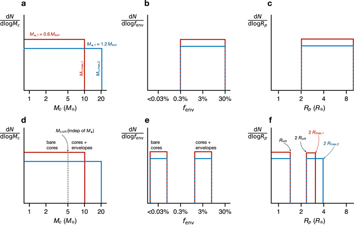
Figure 15. Toy model to explore how a correlation between host star mass M⋆ and planet core mass Mc
impacts super-Earth and sub-Neptune sizes when photoevaporation drives mass loss. Panels (a)–(c) show the distributions of Mc
, envelope fraction fenv, and planet size Rp
at the time of disk dispersal (t ∼ 10 Myr). Here low-mass stars have a lower maximum core mass than high-mass stars: for M⋆ ≈ 0.6 M⊙,  for M⋆ ≈ 1.2 M⊙,
  . Planets have a broad distribution of envelope fractions fenv ≈ 0.3%–30% and a broad distribution of sizes. Panels (d)–(f) show the same properties after the period of rapid photoevaporation (t ∼ 100 Myr). Cores up to Mcrit have been stripped bare. We have approximated the time-integrated XUV flux to be independent of M⋆, so Mcrit is also independent of M⋆ (see Section 8.1). Photoevaporation bifurcates the fenv distribution into two modes with fenv ≈ 0% and 3%. The largest super-Earths have
  , so Rcrit is independent of M⋆. The smallest sub-Neptunes barely retained their envelopes and have Rp
≈ 2Rcrit. The largest sub-Neptune size is set by an fenv ≈ 3% envelope atop an
, so Rcrit is independent of M⋆. The smallest sub-Neptunes barely retained their envelopes and have Rp
≈ 2Rcrit. The largest sub-Neptune size is set by an fenv ≈ 3% envelope atop an  core or
  . Since
  ,
,  . The model is equally applicable to the core-powered framework, except mass is lost over ∼1 Gyr timescales.
Download figure:
Standard image High-resolution imageAfter the period of high XUV activity (t ≳ 100 Myr), cores up to a critical mass Mc,crit are stripped bare, and the largest super-Earth is given by  . Cores above Mc,crit retain their envelopes, and mass loss concentrates envelope fractions to fenv ≈ 3%. The smallest sub-Neptunes have cores that barely retained their envelopes and obey
  the largest sub-Neptunes have an fenv ≈ 3% envelope atop an
  core and obey
  .
.
This toy model reproduces some, but not all, of the observed trends. Here  , so
, so  , which is consistent with the observed trend. Moreover, approximating
  as constant over our mass range predicts a constant
  for different M⋆.
The fact that  R⊕ implies Mc,crit ≈ 8 M⊕ and
  R⊕. Given our assumed
  , we find
  and 4.2 R⊕. While these have the appropriate dependence on M⋆, they exceed the upper envelope of the observed sub-Neptunes. Note, however, that these sizes are at t ∼ 100 Myr, and the observed planets are t ≈ 1–10 Gyr and will contract as they radiate away their heat of formation. Gupta & Schlichting (2020) found that the radius of the radiative–convective boundary (RCB) shrinks as
  . So, over
  = 8–9.7, we expect the planets to shrink by 0.17 dex or 33%. The largest sub-Neptunes would shrink to 2.2 and 2.8 R⊕ for the M⋆,1 ≈ 0.6 and M⋆,2 ≈ 1.2 M⊙ populations, respectively, in rough agreement with observations. However, we note that we observed no age dependence in the mean sub-Neptune size over
  = 9–10, and we comment on this discrepancy later.
Given the similarities between the core- and XUV-powered models, this toy model may be easily adapted to the core-powered model. The key difference is that the time of rapid mass loss is t ≲ 1 Gyr, as opposed to t ≲ 100 Myr.
To summarize, the Rp
–M⋆ correlation observed for super-Earths and sub-Neptunes is broadly consistent with a maximum core mass that increases with M⋆. The  trend suggests an Mc
∝ M⋆ relationship. A linear relationship between core mass and host star mass has also been suggested by Wu (2019) and Berger et al. (2020a).
trend suggests an Mc
∝ M⋆ relationship. A linear relationship between core mass and host star mass has also been suggested by Wu (2019) and Berger et al. (2020a).
Why should core mass increase with host star mass? One explanation could be that the core formation process is dust-limited and that the available dust mass Mdust grows with stellar mass. Pascucci et al. (2016) derived Mdust in protoplanetary disks from ALMA observations at ∼1 mm and found a superlinear relationship with stellar mass  with a large 0.8 dex dispersion about this relationship. It is not clear, however, if core formation is dust-limited due to the difficulties of inferring the total inventories of solids from millimeter emission. Wu (2019) offered a different interpretation, positing that planet cores form at a “thermal mass” Mth, the mass at which a planet’s Hill sphere equals the disk scale height,
  , which is close to the inferred Mc
∝ M⋆ dependence.
, which is close to the inferred Mc
∝ M⋆ dependence.
8.2. Absence of Size–Metallicity Trend Suggests Weak Connection between Envelope Opacity and Stellar Metallicity
Models of sub-Neptunes depend on the envelope opacity κ, which sets the cooling rate and location of the RCB and thus the planet’s size. Higher-opacity envelopes cool and contract more slowly.
In their core-powered models, Gupta & Schlichting (2020) assumed κ ∝ Z, where Z is the bulk stellar metallicity. To isolate the effects of metallicity, they constructed a population of planets with M⋆ fixed at 1.0 M⊙ and [Fe/H] ranging from −0.5 to +0.5 and evolved them for 3 Gyr. The final population is shown in their Figure 9 and reproduced here in Figure 16. In the models, sub-Neptune size increases with stellar metallicity as Rp ∝ Zβ , with β = 0.1. In contrast, in Section 6.2, we measured β = −0.01 ± 0.02, which rules out the predicted β = 0.1 at 4σ significance.
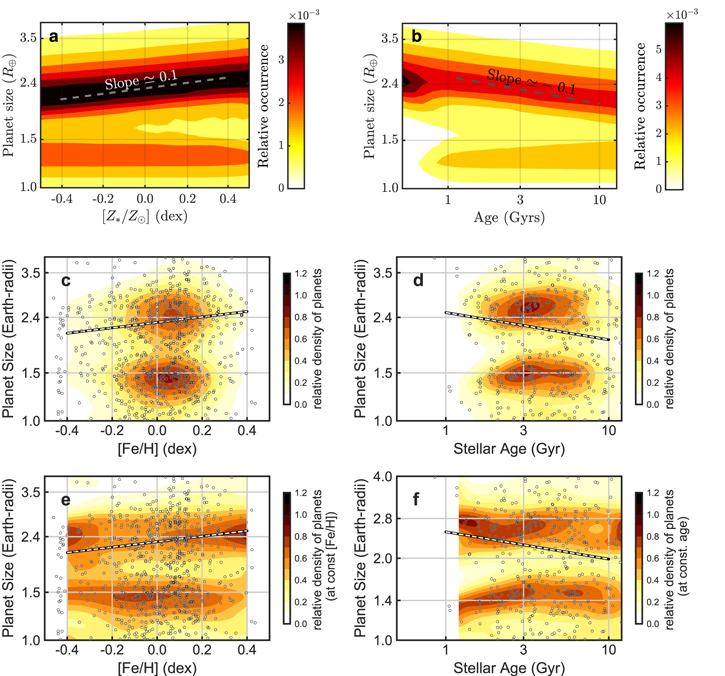
Figure 16. Panel (a): predicted planet sizes as a function of stellar metallicity in the core-powered models of Gupta & Schlichting (2020). Here M⋆ and age were fixed at 1.0 M⊙ and 3 Gyr. Panel (c): relative number density of detected planets (not occurrence). Panel (e): same as panel (c), except we have normalized the number density by its integral along columns of constant [Fe/H] to accentual features at low/high [Fe/H]. In the Gupta & Schlichting (2020) models, the typical sub-Neptune is expected to grow with metallicity according to Rp ∝ Zβ , with β = 0.1. We observed β = −0.01 ± 0.02 and show the predicted β = 0.1 dependence for comparison in panels (c) and (e). The lack of detectable variation in sub-Neptune size with metallicity when such a trend is predicted in the core-powered models points to missing or incomplete physics, perhaps involving the treatment of envelope opacity (see Section 8.2). Panel (b): same as panel (a) except that M⋆ and [Fe/H] were fixed to 1.0 M⊙ and 0.0 dex, and age was allowed to vary. Panels (d) and (f): same as panels (c) and (e) except for age. The sub-Neptunes are expected to shrink with time according to Rp ∝ tγ , with γ = −0.1. While we observed γ = −0.01 ± 0.03, we could not conclusively rule out a γ = −0.1 dependence given the age uncertainties (see Section 8.3).
Download figure:
Standard image High-resolution imageFor visual comparison, we reproduced Figure 7(d) in Figure 16 with a β = 0.1 relationship overplotted. The CXM distribution is peaked near [Fe/H] = 0.0, but no tilt is observable. To visually enhance the tails of the metallicity distribution, we normalized the density by the integrated density along vertical columns. Both super-Earths and sub-Neptunes show no significant size–metallicity dependence.
Our results suggest that the dominant opacity at the RCB does not track stellar metallicity. The tension between the observations and the Gupta & Schlichting (2020) model does not reflect an insurmountable obstacle for core-powered theory but does suggest a modification to the opacity treatment. We also note that the XUV-powered models of Owen & Wu (2017) also assumed a κ ∝ Z relationship.
8.3. Age Effects
After the period of rapid mass loss, we expect the sizes of the sub-Neptunes to decrease due to the Kelvin–Helmholtz mechanism. In Section 6.2, we found Rp ∝ (age/5 Gyr)γ with γ = −0.01 ± 0.03, consistent with no Rp –age collocation. This flat age dependence is interesting given that several studies have noted that planets younger than 100 Myr seem to have inflated envelopes. In a recent compilation of nine planets with cluster-based ages under 100 Myr by Bouma et al. (2020), all were between 4 and 10 R⊕. Rizzuto et al. (2018) and David et al. (2019) made a similar observation among earlier compilations.
Planets in this size range are intrinsically rare among field-age stars. As a point of reference, for P < 100 days, Petigura et al. (2018a) measured an occurrence rate of 0.04 planets star–1 with Rp = 4.0–11.3 R⊕ versus 0.64 planets star–1 with Rp = 1–4 R⊕ among stars with M⋆ ≈ 0.8–1.3 M⊙. Yet V1298 Tau, a 20–30 Myr solar-mass star, hosts four planets with sizes ranging from 5 to 10 R⊕ (David et al. 2019). Planets in this size range are even rarer among low-mass stars. Dressing & Charbonneau (2013) measured an occurrence rate of 0.007 planets star–1 with Rp = 4.0–11.3 R⊕ and P < 50 days in a sample of stars with M⋆ ≈ 0.4–0.6 M⊙. Yet K2-33 is a 5–10 Myr, 0.4 M⊙ star that hosts a 6 R⊕ planet (David et al.2016).
Given the evidence for inflated planets younger than 100 Myr in the literature combined with the flat Rp –age relationship observed here for ages spanning 1–10 Gyr, we conclude that large-scale evolution in the size of sub-Neptune envelopes concludes by ∼1 Gyr.
The envelopes may continue to contract after ∼1 Gyr, but the Rp –age trends may be too subtle to detect given our sample size and age uncertainties. For example, Gupta & Schlichting (2020) isolated the age effect in the core-powered context by constructing a planet population with M⋆ and [Fe/H] held fixed at 1.0 M⊙ and 0.0 dex and evolved them from 1 to 10 Gyr (their Figure 10, reproduced here in Figure 16). In this model, the planets obeyed a γ = −0.1 relationship. However, errors in the measured ages will conspire to flatten such a trend. We explored this effect by injecting a γ = −0.1 dependence into the observed sub-Neptune population, perturbing their ages by their uncertainties, and refitting our power-law model. We found γ = −0.06, which is consistent with our measured value of γ = −0.01 ± 0.03 at the 2σ level. Thus, we cannot rule out the subtle γ = −0.1 dependence predicted by Gupta & Schlichting (2020) given our current sample size and age uncertainties.
8.4. Slope of the Radius Gap in Period–Radius Space
While a number of theoretical models can produce the radius gap, they do not produce identical slopes in the P–Rp plane. Thus, the slope of the radius gap has emerged as a potential discriminant between different models. In the Owen & Wu (2017) photoevaporation model, the maximum size of a super-Earth decreases with orbital period. The upper envelope is set by the size of a rocky core that is barely stripped by the integrated XUV exposure. Slightly more massive cores retain their envelopes and remain sub-Neptunes.
At larger orbital periods,  decreases, and the cores that can be completely stripped have lower masses and smaller sizes. Assuming a fixed energy-limited efficiency factor η = 10%, Owen & Wu (2017) predicted that the bottom of the radius gap will follow Rp
∝ Pm
with m = −0.25. Realistically, η should decline as mass increases, since escaping gas has more time to cool as it climbs out of a deeper potential well. Adopting
decreases, and the cores that can be completely stripped have lower masses and smaller sizes. Assuming a fixed energy-limited efficiency factor η = 10%, Owen & Wu (2017) predicted that the bottom of the radius gap will follow Rp
∝ Pm
with m = −0.25. Realistically, η should decline as mass increases, since escaping gas has more time to cool as it climbs out of a deeper potential well. Adopting  yields a shallower slope, m = −0.16.
In the core-powered framework of Gupta & Schlichting (2019), the fate of an envelope around a planet with P ≳ 8 days depends on the cooling timescale tcool = E/L relative to the envelope mass-loss timescale  . Envelopes that escape faster than they cool, tloss < tcool, are lost completely. The mass-loss timescale depends on
  at the Bondi radius, and
  , where Rs
is the sonic point and cs
is the sound speed. The cooling timescale may be computed by dividing the combined thermal and gravitational energy of the envelope and core by the luminosity evaluated at the RCB. The exponential behavior of tloss results in the dividing line tloss = tcool being set by
, where Rs
is the sonic point and cs
is the sound speed. The cooling timescale may be computed by dividing the combined thermal and gravitational energy of the envelope and core by the luminosity evaluated at the RCB. The exponential behavior of tloss results in the dividing line tloss = tcool being set by  , which implies Rp
∝ P−0.11 or m = −0.11.
, which implies Rp
∝ P−0.11 or m = −0.11.
We emphasize that the values of m predicted by the core- and XUV-powered models discussed above have all incorporated assumptions about the properties of planet cores, such as the distribution of masses, orbital periods, and bulk compositions. Rogers et al. (2021) showed how changing these input parameters can alter the predicted m. However, both the core- and XUV-powered models categorically predict a negative slope.
Models that delay the accretion of gas until the nebula is nearly or completely dissipated predict an increasing slope with orbital period. Here the core mass is determined by the solid surface density profile within a feeding zone that is proportional to the Hill radius  . A Hayashi (1981) profile Σ(a) ∝ a−3/2 yields
  ,
,  , or m = 0.11.
For the full CXM sample, we measured m =  . Van Eylen et al. (2018) fit the gap in a sample of 117 planets orbiting 75 stars with asteroseismic detections and found m =
  . Their population of stellar hosts most closely resembles a combination of our middle- and high-mass bins, for which we measured m =
  and
and  , which straddle the Van Eylen et al. (2018) value. Martinez et al. (2019) performed an independent analysis of CKS DR1 spectra including parallax constraints and found m = −0.11 ± 0.02. Despite differences in the planets used, planet/star parameter provenance, and slope measurement technique, our measurements of slope are consistent with the Van Eylen et al. (2018) and Martinez et al. (2019) measurements and the core- and XUV-powered model predictions.
Shifting our attention to low-mass stars, we resolved the radius gap among the 185 planets in our low stellar mass bin M⋆ = 0.5–0.7 M⊙. We measured m =  , consistent with that of the full sample. As a point of comparison, Cloutier & Menou (2020) measured the occurrence of planets in a sample of stars having Teff < 4700 K drawn from Kepler and K2 (275 and 53 planets). The host stars were M⋆ = 0.08–0.93 M⊙, but most were between 0.5 and 0.8 M⊙. They resolved the radius gap and measured a positive slope in P–Rp
space of m = 0.058 ± 0.022. They interpreted this as a signature of gas-poor formation channels around lower-mass stars. However, the radius gap is only visible in their full 328-planet sample, but not when they restrict their analysis to the 126 planets around M⋆ = 0.08–0.65 M⊙ hosts (their Figure 12). Our measured slope is ≈4σ lower than that of Cloutier & Menou (2020). We found no evidence of a change of slope and thus do not favor an alternate formation pathway for planets around M⋆ = 0.5–0.7 M⊙ stars. Van Eylen et al. (2021) arrived at a similar conclusion after analyzing a sample of 27 planets orbiting stars with Teff < 4000 K.
, consistent with that of the full sample. As a point of comparison, Cloutier & Menou (2020) measured the occurrence of planets in a sample of stars having Teff < 4700 K drawn from Kepler and K2 (275 and 53 planets). The host stars were M⋆ = 0.08–0.93 M⊙, but most were between 0.5 and 0.8 M⊙. They resolved the radius gap and measured a positive slope in P–Rp
space of m = 0.058 ± 0.022. They interpreted this as a signature of gas-poor formation channels around lower-mass stars. However, the radius gap is only visible in their full 328-planet sample, but not when they restrict their analysis to the 126 planets around M⋆ = 0.08–0.65 M⊙ hosts (their Figure 12). Our measured slope is ≈4σ lower than that of Cloutier & Menou (2020). We found no evidence of a change of slope and thus do not favor an alternate formation pathway for planets around M⋆ = 0.5–0.7 M⊙ stars. Van Eylen et al. (2021) arrived at a similar conclusion after analyzing a sample of 27 planets orbiting stars with Teff < 4000 K.
Before concluding this section, we wish to remark on some of the challenges associated with using the slope of the radius gap as a signpost of formation. Note that our uncertainties on m are larger than those of Martinez et al. (2019), even though we resolved the valley at higher contrast (compare our Figure 7 to their Figure 12). One may understand this through the following limiting case. Consider super-Earth/sub-Neptune populations separated by a gap completely devoid of planets. In such a scenario, selecting the minima used to fit the radius gap in Section 6.1 is ill-poised because there is no longer a single minimum Rp . Thus, a broad range of Rp,0 and m are allowed. Thus, the statistic for assessing model predictions has the undesirable quality of becoming more uncertain as observational uncertainties improve.
Moreover, there is no standard approach to fitting the absence of planets. For example, Van Eylen et al. (2018) used a support vector machine scheme, Berger et al. (2020a) used the “gapfit” code that subtracts off a trial Rp ∝ Pm relationship and evaluates a 1D KDE of the residuals, and Martinez et al. (2019) and this work fit a train of minima computed along 1D projections through the P–Rp plane. All approaches rely on an ad hoc smoothing parameter that determines the relative influence of the few planets near the edge of the gap relative to the many planets far from the gap on the fit. These differences in fitting method are less troublesome in theoretical studies that can model limitless numbers of planets and do not contend with complications like false-positive contamination or mischaracterized measurement uncertainties.
Recently, Rogers & Owen (2021) introduced a different framework for evaluating the agreement between formation theory and the observed planet population that does not rely on measuring the slope of the gap. Here a model planet population is subjected to a specified set of physical processes, e.g., XUV- or core-powered mass loss. The synthetic population is transformed into an ORD distribution. This is then converted into a number rate density distribution by accounting for properties of the parent stellar population and losses due to nontransiting planets and pipeline incompleteness. In this framework, one evaluates the likelihood that the observed planets are a realization of an inhomogeneous Poisson point process with the specified number rate density. One may then optimize the model parameters and characterize their uncertainties using standard techniques. Such a treatment of the CXM sample would be interesting but is beyond the scope of this paper.
8.5. Period–Flux Distribution of Planets
In Section 7.3, we characterized the period distribution of super-Earths and sub-Neptunes  in three bins of stellar mass. We parameterized these distributions as smooth broken power laws with variable breakpoints P0. From M⋆ = 0.5 t0 1.4 M⊙, the sub-Neptune falloff occurs at a nearly constant P0 ≈ 10 days. Similarly, when we modeled the flux distribution,
  , we found that Sinc,0 increases by nearly an order of magnitude, from ≈20 to 200 S⊕.
Under the assumptions that planet cores (1) are uniformly distributed in log-period and (2) have masses that are uncorrelated with M⋆, the above observation would be strong evidence for XUV-powered and against core-powered mass loss. As we explain in Section 8.1,  and thus only varies by 40% over our full mass stellar range. Thus, the critical
  that strips the typical sub-Neptune maps to a P0 that is constant with M⋆. A fixed P0 corresponds to an Sinc,0 that grows with M⋆. Under the same assumptions, Sinc,0 should be constant with M⋆ in the core-powered model.
Neither of the above assumptions, however, appear to be correct. The steep decline in super-Earths for P ≲ P0 ≈ 5 days suggests that rocky cores struggle to form inside this boundary. Several mechanisms may be responsible, including magnetospheric truncation of the inner disk (e.g., Lee & Chiang 2017) or a pressure trap due a silicate sublimation front (e.g., Flock et al. 2019). Moreover, the M⋆–Rp correlation discussed in Section 8.1 suggests that massive stars make massive cores.
Therefore, we cannot rule out the core-powered model based on the dependence of P0 and Sinc,0 on M⋆. In this framework, stars that are 1.0–1.4 M⊙ efficiently produce sub-Neptunes when Sinc ≲ Sinc,0 ≈ 200 S⊕. Stars that are 0.5–0.7 M⊙ only efficiently produce sub-Neptunes when Sinc ≲ Sinc,0 ≈ 20 S⊕. The lack of sub-Neptunes in the Sinc ≈ 20–200 S⊕ range is not due to envelope stripping but rather to the absence of suitable cores. Inspecting Figure 13, we see that the ORD of super-Earths declines by a factor of 5 over Sinc = 20–200 S⊕.
There is still considerable uncertainty in the distribution of core masses and further uncertainty in how that distribution varies with P and M⋆. Given these unknowns, both core- and XUV-powered frameworks appear sufficiently flexible to match the observations. Additional mass measurements of sub-Neptunes as a function of P–Sinc–M⋆ should help to constrain the models, since Rp and Mp together constrain both core mass and envelope fraction.
9. Summary and Conclusion
Here we provide a brief summary of our results and point toward future improvements to this work.
- 1.We augmented the 1305-star CKS DR1 spectral library with DR2 containing 411 new spectra.
- 2.We performed a homogeneous analysis of the combined DR1 and DR2 samples and derived Teff, [Fe/H],, M⋆, R⋆, and age.
- 3.We constructed a curated sample of 970 planets orbiting 703 stars with updated star/planet properties.
- 4.We resolved the radius gap and projected the planet population as a function of P, Sinc, M⋆, [Fe/H], and age.
- 5.The radius gap in the P–Rp plane follows Rp ∝ Pm with m = −0.10 ± 0.03, consistent with both core- and XUV-powered models but inconsistent with gas-poor formation models.
- 6.We observed no significant change in m over 0.5–1.4 M⊙.
- 7.Sub-Neptunes tend to be larger around higher-mass stars and follow with α = 0.25 ± 0.03. The super-Earths exhibit no measurable M⋆ dependence α = 0.02 ± 0.03. Taken together, these trends are consistent with a core mass distribution that scales linearly with stellar mass Mc
∝ M⋆.
- 8.The average sub-Neptune is not measurably larger around higher-metallicity stars, disfavoring a simple linear relationship between envelope opacity and stellar metallicity κ ∝ Z.
- 9.The average sub-Neptune does not measurably shrink over 1–10 Gyr. Given the large radii observed among stars younger than 100 Myr, we conclude that the majority of planet radius contraction concludes by ∼1 Gyr.
- 10.The period distribution of sub-Neptunes has a breakpoint P0 in M⋆. This is consistent with the predictions of photoevaporation models. However, core-powered models may still be viable given the uncertainties in the underlying distribution of planet cores.


The bifurcation of small planets into two distinct populations was one of the most intriguing results from the Kepler mission. This feature appears most consistent with models where close-in planets acquire and lose H/He envelopes. The XUV radiation from young stars or heat from cooling cores are leading candidates for the energy source that powers this mass loss. While we worked to identify the dominant mass-loss process, we found that both mechanisms are flexible enough to match our observations.
We look forward to additional observational and theoretical work that could help discriminate between these two theories. With Gaia, it will soon be possible to extend the analysis presented here to a larger sample of planets (2–3×). Future Gaia data releases will include low- and high-resolution spectra for nearly all Kepler stars. These data will increase the upper M⋆ limit, since rapid rotation above 6500 K does not wash out broadband spectral energy distribution information. Gaia-based refinements in Teff and [Fe/H] will be especially useful in determining masses and ages for additional early-type stars. However, increases in sample size from Gaia may not settle the core-powered versus XUV-powered question. An analysis of synthetic planet populations by Rogers et al. (2021) suggested that ≳5000 planets are needed to do so.
We found that heuristic descriptions of the radius gap, such as its slope in the P–Rp plane, were neither straightforward to compute nor straightforward to compare to model predictions, which are based on a previous occurrence analysis. The disconnect between the demographic analysis and the population modeling leads to concerns of self-inconsistency. The modeling approach of Rogers & Owen (2021) offers a firmer statistical basis for comparing models and observations. This approach can also naturally accommodate realistic nonindependent distributions of host star properties like mass, metallicity, and age.
Aside from improved host star properties, additional planet observables should shed light on the mass-loss process. Mass measurements of transiting planets spanning P, Sinc, [Fe/H], and age will help constrain the core mass distribution that contributes to the remaining flexibility of both models, since mass and radius together constrain core mass and envelope fraction. Finally, direct measurements of mass loss as a function of the same properties would be especially valuable. Outflows from a handful of planets have been recently detected using the He 10830 Å line, and Gupta & Schlichting (2021) have highlighted a number of planets that may actively be experiencing mass loss in the core-powered framework.
We thank Natalie Batalha, Konstantin Batygin, Akash Gupta, Daniel Huber, Eric Lopez, Hilke Schlichting, Joshua Schlieder, Samuel Yee, and Jon Zink for valuable conversations that improved this manuscript.
The data presented herein were obtained at the W. M. Keck Observatory from telescope time allocated to the National Aeronautics and Space Administration through the agency’s scientific partnership with the California Institute of Technology and the University of California. The Observatory was made possible by the generous financial support of the W. M. Keck Foundation.
Kepler was competitively selected as the 10th NASA Discovery mission. Funding for this mission is provided by the NASA Science Mission Directorate. We thank the Kepler Science Office, the Science Operations Center, the Threshold Crossing Event Review Team (TCERT), and the Follow-up Observations Program (FOP) working group for their work on all steps in the planet discovery process, ranging from selecting target stars to curating planet catalogs.
E.A.P. acknowledges support from the following sources: Hubble Fellowship grant HST-HF2-51365.001-A awarded by the Space Telescope Science Institute, which is operated by the Association of Universities for Research in Astronomy, Inc., for NASA under contract NAS 5-26555; a NASA Keck PI Data Award (80NSSC20K0308), administered by the NASA Exoplanet Science Institute; a NASA Astrophysics Data Analysis Program (ADAP) grant (80NSSC20K0457); and the Alfred P. Sloan Foundation.
The authors wish to recognize and acknowledge the very significant cultural role and reverence that the summit of Maunakea has long had within the indigenous Hawaiian community. We are most fortunate to have the opportunity to conduct observations from this mountain.
Facilities: Keck:I (HIRES) - , Kepler. -
Software: The software used in this analysis is available on GitHub (https://github.com/petigura/CKS-Cool) and archived on Zenodo (Petigura & Rogers 2022). We used the following additional packages: Astropy (Astropy Collaboration et al. 2013), emcee (Foreman-Mackey et al. 2013), isoclassify (Huber et al. 2017; Berger et al. 2020b), Lmfit (Newville et al. 2014), Matplotlib (Hunter 2007), Numpy (van der Walt et al. 2011), Scipy (Jones et al. 2001), H5py (Collette et al. 2021), Pandas (McKinney 2010), Seaborn (Waskom 2021), and Xarray (Hoyer & Hamman 2017).
Footnotes
- 13
NEA data column: koi_pdisposition.
- 14
NEA data column: koi_score.
- 15
NEA data column: koi_pdisposition.
- 16
NEA data column: koi_max_mult_ev.
- 17
NEA data column: koi_fittype.
- 18
- 19
- 20
- 21
The normalization constant C is
where 2 F1 is the hypergeometric function.
