Abstract
The PHANGS project is assembling a comprehensive, multiwavelength data set of nearby (∼5–20 Mpc), massive star-forming galaxies to enable multiphase, multiscale investigations into the processes that drive star formation and galaxy evolution. To date, large survey programs have provided molecular gas (CO) cubes with the Atacama Large Millimeter/submillimeter Array, optical integral field unit (IFU) spectroscopy with the Very Large Telescope/Multi-Unit Spectroscopic Explorer (MUSE), high-resolution near-ultraviolet–optical imaging in five broadband filters with Hubble Space Telescope (HST), and infrared imaging in NIRCAM+MIRI filters with JWST. Here we present PHANGS-HST-Hα, which has obtained high-resolution (∼2–10 pc), narrowband imaging in the F658N or F657N filters with the HST/WFC3 camera of the warm ionized gas in the first 19 nearby galaxies observed in common by all four of the PHANGS large programs. We summarize our data reduction process, with a detailed discussion of the production of flux-calibrated, Milky Way extinction-corrected, continuum-subtracted Hα maps. PHANGS-MUSE IFU spectroscopy data are used to background-subtract the HST-Hα maps and to determine the [N ii] correction factors for each galaxy. We describe our public data products (the data released as part of this work include the reduced drizzled narrowband images and the flux-calibrated, continuum-subtracted Hα maps for each galaxy; these images are available for download via MAST at https://archive.stsci.edu/hlsp/phangs.html, as well as at the Canadian Astronomy Data Centre as part of the PHANGS archive at https://www.canfar.net/storage/vault/list/phangs/RELEASES) and highlight a few key science cases enabled by the PHANGS-HST-Hα observations.
Original content from this work may be used under the terms of the Creative Commons Attribution 4.0 licence. Any further distribution of this work must maintain attribution to the author(s) and the title of the work, journal citation and DOI.
This article was updated on April 7, 2025 to correct a production error which led to incorrect text citations for some references.
1. Introduction
The warm ionized gas within galaxies plays a pivotal role in shaping their morphology and evolution. Discrete structures of ionized gas include H ii regions/complexes, planetary nebulae (PNe), and supernova remnants (SNRs), among others. In addition to Hα emission originating from H ii regions, some ionizing photons escape and can travel far from their birth sites into lower-density material. This diffuse ionized gas (DIG) can contribute a significant fraction of the total Hα emission from spiral galaxies and offers insights into interstellar radiation transport and its broader environmental impact. Recent advances, notably through instruments like the Multi-Unit Spectroscopic Explorer (MUSE), have revolutionized our ability to study the distribution and properties of the low surface brightness DIG (e.g., R. A. M. Walterbos & R. Braun 1994; F. Belfiore et al. 2022), shedding light on its connection to stellar feedback processes.
The evolution in the size of H ii regions is critical as a diagnostic of stellar feedback, which is viewed as one of the most important but uncertain aspects of galaxy evolution. Feedback from massive stars (e.g., winds, radiation, supernovae) in clusters and associations exerts pressure on the surrounding natal gas and dust, initiating a dynamic evolution from classic Strömgren spheres (on scales of order a parsec) to larger bubbles and even the most massive superbubble structures, such as the ∼kiloparsec-size Phantom Void (A. T. Barnes et al. 2023). The dominant feedback mechanism changes as a function of time and spatial scale (e.g., D. Rahner et al. 2017; M. Chevance et al. 2020; G. M. Olivier et al. 2021), with radiation pressure playing an important role early on. As ionizing photons penetrate the surrounding material, they create overpressured expanding regions of ionized gas, characterized by bubbles, perforated walls, and partial shells. The morphology of these structures, including their radius, degree of perforation/irregularity, and hierarchical organization, reflects the complex interplay between stellar feedback and the surrounding interstellar medium (ISM; e.g., L. M. Haffner et al. 2009).
For galaxies at distances of ≈5–20 Mpc, it is challenging to identify and study individual H ii regions, since ground-based resolution is typically limited to ≈1″ (≈50–100 pc; A. F. McLeod et al. 2020; A. T. Barnes et al. 2021) and compact H ii regions observed in the Milky Way have scales of just a few parsecs or below (J. L. Caswell & R. F. Haynes 1987; E. Churchwell 2002; L. D. Anderson et al. 2014). By obtaining more detailed maps of Hα emission at these spatial scales, we will be able to connect individual stellar sources of ionization to the ionized gas and study the structure of feedback-dominated regions in detail, including shells, partial shells driven by H ii regions, or larger bubbles propelled by supernova contributions, as well as assessing the sources of previously identified faint emission features, such as DIG. In all, new high-resolution observations will enable us to close the loop on the impact of stellar feedback on galaxy-wide evolution from the stellar sources to their influence on the surrounding ISM, the formation and evolution of structures such as bubbles, and their influence on the subsequent generation(s) of stars. This is now particularly relevant in the era of subarcsecond-resolution (∼Hubble Space Telescope (HST) matched) studies of the ISM offered by the James Webb Space Telescope (JWST).
The Cycle 30 HST Treasury project, PHANGS-HST-Hα, provides high-resolution maps of Hα emission across 19 nearby spiral galaxies observed as part of the Physics at High Angular Resolution in Nearby Galaxies (PHANGS) project and is the subject of this work. The multiwavelength data set includes high-resolution CO (2−1) maps from the Atacama Large Millimeter/submillimeter Array (ALMA; A. K. Leroy et al. 2021), broadband imaging in 14 filters (including the Hα presented here) from the near-ultraviolet (NUV) through the mid-infrared with HST (J. C. Lee et al. 2022) and JWST (J. C. Lee et al. 2023; T. G. Williams et al. 2024), and optical integral field unit (IFU) spectroscopy with the Very Large Telescope (VLT)/MUSE (E. Emsellem et al. 2022).
In this paper, we present the design of the PHANGS-HST-Hα survey, provide an overview of the data processing pipeline, and describe the data products made public to the community. The remainder of this paper is organized as follows: In Section 2 we present the basic properties of our sample galaxies. Section 3 summarizes the new HST data and reduction, as well as key characteristics of the MUSE/IFU spectra, which are used to improve the flux calibration of the HST images. Next, we explain in detail the flux calibration, continuum subtraction, and correction for [N ii] emission of the PHANGS-HST-Hα images (Section 4; see flowchart in Figure 4). We make the PyHSTHAContSub30 pipeline for producing the flux-calibrated, continuum-subtracted images publicly available online.31 Section 5 presents the reduced data products and highlights key science areas where the Hα maps will provide critical input. We summarize the key points of our work in Section 6, including information on upcoming data products.
2. Galaxy Sample
The PHANGS multiwavelength surveys focus on nearby, massive, and relatively face-on spiral galaxies. The parent sample (74 galaxies), described in A. K. Leroy et al. (2021), selected spirals visible from the southern hemisphere (i.e., observable by ALMA and the VLT) and within ≈20 Mpc that have an inclination less than 75∘. The distance selection ensures that HST and JWST can resolve individual star clusters and associations, that MUSE can identify H ii regions, and that ALMA resolves the ISM into molecular clouds and cloud complexes. In order to focus on galaxies on the star-forming “main sequence,” the environments where most massive stars form at z = 0 (J. Brinchmann et al. 2004; S. Salim et al. 2007; R. Genzel et al. 2010; A. Saintonge et al. 2017), the survey also selected galaxies with a stellar mass higher than 5 × 10⁹ M⊙ and a specific star formation rate (SFR/M*) ≥ 10−11 yr−1.
Here we present an overview of the PHANGS-HST-Hα Treasury survey. This project targets the 19 galaxies observed as part of the PHANGS-JWST Treasury program (PI: J. Lee); NGC 628, NGC 4254, and NGC 5068 have two pointings, for a total of 22 fields. All target galaxies have high-resolution imaging from HST available in five UV through optical broad bands (PHANGS-HST; PI: J. Lee), millimeter-wave spectral mapping from PHANGS-ALMA (A. K. Leroy et al. 2021), and ground-based optical IFU spectroscopy from VLT/MUSE (E. Emsellem et al. 2022), as well as many other multiwavelength observations. The basic properties of the galaxies, including distance, SFR (total and that in the area covered by the HST observations), and stellar mass, are listed in Table 1. Figure 1 shows BVI+Hα color images for the 17 out of 19 target galaxies that currently have Hα images available. Young, recently formed stars appear blue; the pinkish-red emission shows the warm ionized gas that is the focus of this work.
Table 1. Properties of PHANGS-HST-Hα Galaxies
| Galaxy | α | δ | Distance | SFRtot | SFR | log M* | log10LCO |
|---|---|---|---|---|---|---|---|
| (J2000) | (J2000) | (Mpc) | (M⊙ yr−1) | (M⊙ yr−1) | (log M⊙) | (K km s−1 pc2) | |
| (1) | (2) | (3) | (4) | (5) | (6) | (7) | (8) |
| IC 5332 | 23h34m27 49 49 | −36d06m03 9 9 | 9.01 ± 0.41 | 0.41 | 0.11 | 9.5 | 7.1 |
| NGC 628-C* | 01h36m39 82 82 | +15d46m34 6 6 | 9.84 ± 0.63 | 1.75 | 0.93 | 10.3 | 8.4 |
| NGC 628-E | 01h36m41 75 75 | +15d47m01 2 2 | 9.84 ± 0.63 | 1.75 | 0.93 | 10.3 | 8.4 |
| NGC 1087 | 02h46m25 16 16 | −00d29m55 1 1 | 15.85 ± 2.24 | 1.31 | 1.25 | 9.9 | 8.3 |
| NGC 1300* | 03h19m41 08 08 | −19d24m40 9 9 | 18.99 ± 2.85 | 1.17 | 1.02 | 10.6 | 8.5 |
| NGC 1365 | 03h33m36 37 37 | −36d08m25 4 4 | 19.57 ± 0.78 | 16.90 | 12.88 | 11.0 | 9.5 |
| NGC 1385 | 03h37m28 85 85 | −24d30m01 1 1 | 17.22 ± 2.58 | 2.09 | 1.96 | 10.0 | 8.4 |
| NGC 1433* | 03h42m01 55 55 | −47d13m19 5 5 | 18.63 ± 1.86 | 1.13 | 0.56 | 10.9 | 8.5 |
| NGC 1512 | 04h03m54 28 28 | −43d20m55 9 9 | 18.83 ± 1.88 | 1.28 | 0.59 | 10.7 | 8.3 |
| NGC 1566 | 04h20m00 42 42 | −54d56m16 1 1 | 17.69 ± 2.00 | 4.54 | 3.21 | 10.8 | 8.9 |
| *NGC 1672* | 04h45m42 50 50 | −59d14m49 9 9 | 19.40 ± 2.91 | 7.60 | 6.60 | 10.7 | 9.1 |
| NGC 2835-S | 09h17m53 04 04 | −22d23m01 2 2 | 12.22 ± 0.94 | 1.24 | 0.57 | 10.0 | 7.7 |
| NGC 2835-N† | 09h17m53 11 11 | −22d21m19 5 5 | 12.22 ± 0.94 | 1.24 | 0.57 | 10.0 | 7.7 |
| NGC 3351 | 10h43m57 70 70 | +11d42m13 7 7 | 9.96 ± 0.33 | 1.32 | 0.87 | 10.4 | 8.1 |
| NGC 3627 | 11h20m14 96 96 | +12d59m29 5 5 | 11.32 ± 0.48 | 3.84 | 3.31 | 10.8 | 9.0 |
| NGC 4254-E | 12h18m56 16 16 | +14d26m03 5 5 | 13.1 ± 2.8 | 3.07 | 2.77 | 10.4 | 8.9 |
| NGC 4254-W | 12h18m46 80 80 | +14d24m36 9 9 | 13.1 ± 2.8 | 3.07 | 2.77 | 10.4 | 8.9 |
| NGC 4303 | 12h21m54 90 90 | +04d28m25 1 1 | 16.99 ± 3.04 | 5.33 | 4.25 | 10.5 | 9.0 |
| NGC 4321 | 12h22m54 83 83 | +15d49m18 5 5 | 15.21 ± 0.49 | 3.56 | 2.43 | 10.8 | 9.0 |
| NGC 4535 | 12h34m20 36 36 | +08d11m52 1 1 | 15.77 ± 0.37 | 2.16 | 1.23 | 10.5 | 8.6 |
| NGC 5068-N | 13h18m49 68 68 | −21d01m24 8 8 | 5.20 ± 0.21 | 0.28 | 0.20 | 9.4 | 7.3 |
| NGC 5068-S | 13h18m53 92 92 | −21d03m10 4 4 | 5.20 ± 0.21 | 0.28 | 0.20 | 9.4 | 7.3 |
| NGC 7496 | 23h09m47 29 29 | −43d25m40 6 6 | 18.72 ± 2.81 | 2.26 | 2.00 | 10.0 | 8.3 |
Note. Column (1): galaxy name. An asterisk indicates that the HST-Hα observations are archival; a dagger indicates NGC 2835-N was observed just prior to publication, and the images for this galaxy will be included in the next image release. Columns (2)–(3): R.A. and decl. Column (4): distance in Mpc. Columns (5)–(6): SFR for the entire galaxy and the portion in the HST footprint (footprints are shown in the Appendix). Column (7): galaxy stellar mass. Column (8): integrated CO (2–1) luminosity. Scale this by αCO ≈ 6.7M⊙ pc−2 (K km s−1)−1 to estimate the molecular mass.
Download table as: ASCIITypeset image
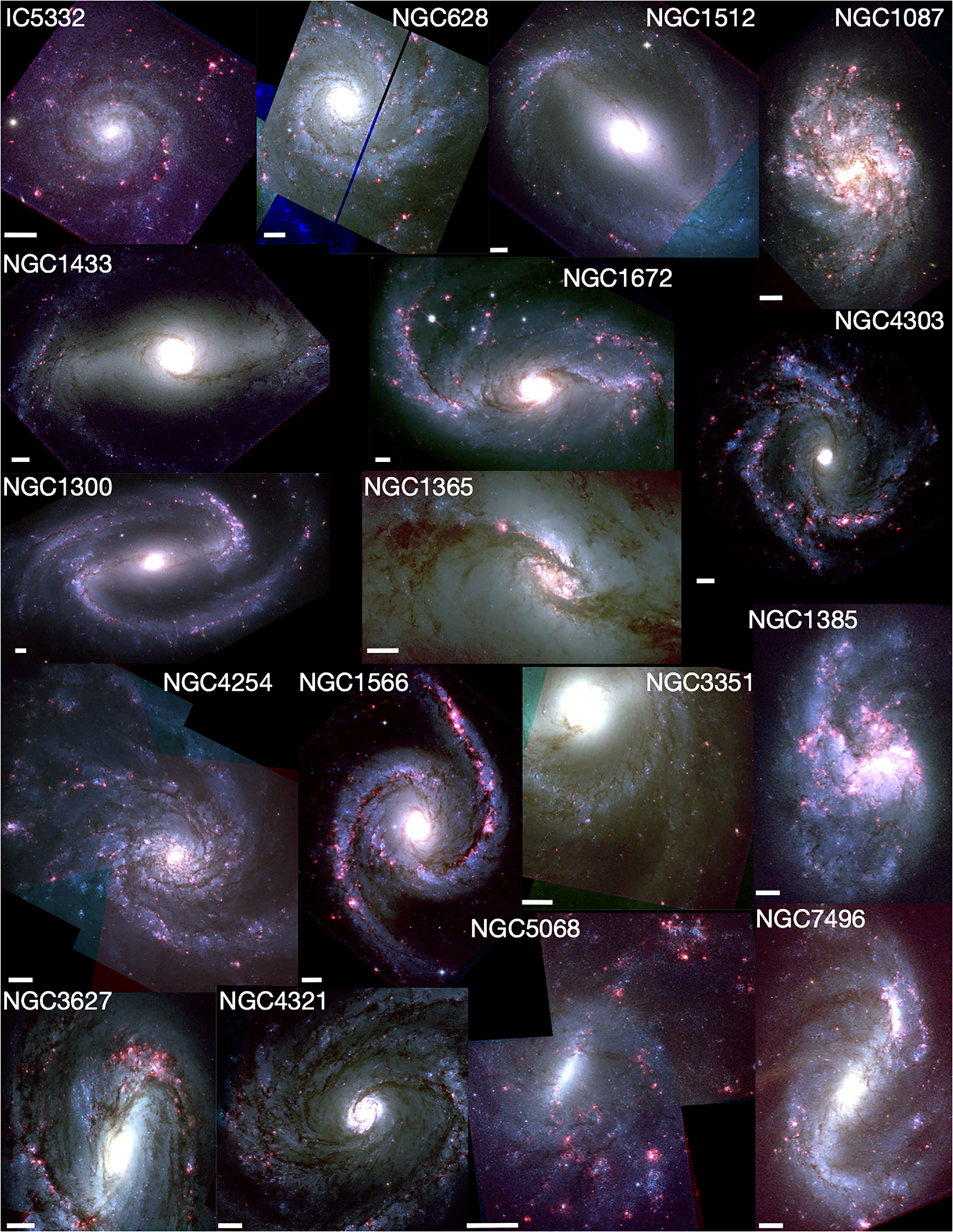
Figure 1. B − V − I+Hα blue–green–red color composite images for the 17 (of 19) galaxies in our sample that have HST-Hα images available at this time. The Hα emission (red) shows the locations of recent (≲6 Myr) star formation. A 1 kpc scale bar is indicated for each galaxy. The images show a variety of environments and morphologies.
Download figure:
Standard image High-resolution imageDistance determinations to the galaxies in the PHANGS-HST-Hα sample are taken from the compilation in G. S. Anand et al. (2021) and are based on a variety of methods. G. S. Anand et al. (2021) determined new distances to six of these galaxies based on the tip of the red giant branch (TRGB). For the rest, they carefully assessed distance estimates available in the literature, which can vary in quality, and assigned an associated uncertainty. Preference was given to high-quality primary indicators such as TRGB or Cepheid-based measurements, followed by estimates from other standard candles such as the PN luminosity function or surface brightness fluctuations. The lowest priority was given to distances based on modeling of local dynamical flows (H. M. Courtois et al. 2012).
Two estimates of the SFR are listed in Table 1. Column (5) compiles the total SFR (SFRtot), which is estimated for the entire galaxy from the far-ultraviolet luminosity measured from Galaxy Evolution Explorer (GALEX) and the infrared luminosity measured from Wide-field Infrared Survey Explorer (WISE) W4 and follows the prescription given in A. K. Leroy et al. (2019), which is calibrated to match the results of the population synthesis modeling given in S. Salim et al. (2016, 2018). Column (6) provides the SFR, computed as for the entire galaxy, but limited to the area covered by the PHANGS-HST footprint (shown in the Appendix), which is similar to that covered by the HST-Hα observations presented here. The stellar mass estimates are from A. K. Leroy et al. (2021) based on IRAC 3.6 μm observations when available and WISE W1 3.4 μm maps otherwise. There is significant overlap in the wavelength coverage of the two bands, and both should be dominated by the light from old stars with little impact from dust extinction. The near-infrared luminosity is combined with radially varying mass-to-light ratios, which are determined from constraints on the stellar population in each galaxy, to calculate the total stellar mass. These values are compiled in Column (7) of Table 1. In Column (8) we compile the integrated CO (2–1) luminosity for each galaxy from A. K. Leroy et al. (2023). The total mass of molecular gas Mmol can be estimated by assuming a fixed CO-to-H2 conversion factor of αCO ≈ 6.7M⊙ pc−2 (K km s−1)−1.
Figure 2 shows basic properties of the PHANGS-HST-Hα sample relative to the total PHANGS sample and to nearby star-forming galaxies in general. The left panel of Figure 2 shows M* versus SFR for galaxies in the larger PHANGS sample and in the PHANGS-HST-Hα subsample, overlaid on the locus occupied by star-forming galaxies from the Sloan Digital Sky Survey (SDSS; S. Salim et al. 2016). The PHANGS samples provide excellent coverage of the main sequence located between stellar masses of ∼109.5 and 1011 M⊙. Main-sequence galaxies in this stellar mass range are representative of the galaxies where the bulk of present-day star formation is taking place (S. Salim et al. 2007; A. Saintonge et al. 2017). The HST-Hα subsample is weighted toward galaxies with somewhat higher SFR. Ongoing HST observations (see Section 3.1) will provide Hα and NUV − U − B − V − I HST imaging for a combined total of 74 PHANGS galaxies, removing this bias. The right panel of Figure 2 shows ΣSFR (SFR per area) as a function of the molecular gas surface density for the full PHANGS sample (open circles) and for the PHANGS-HST-Hα subsample (red plus signs).
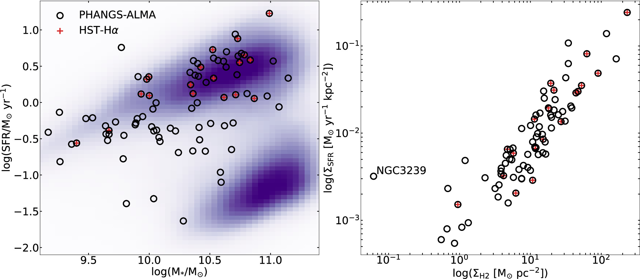
Figure 2. Left: galaxies from the SDSS sample with z ≲ 0.1 form the backdrop of the left panel, where the galaxy star-forming sequence is the prominent upper feature. Coverage of the SFR–M* plane by galaxies in the parent PHANGS sample (N = 74; open circles) is shown. Red plus signs show that the 19 galaxies observed as part of the HST-Hα project tend to have higher SFRs. Right: the star formation and molecular gas surface brightness (J. Sun et al. 2022) for the parent PHANGS sample (open circles) and the PHANGS-HST-Hα subsample studied here (red plus signs). Outlier NGC 3239 is noted.
Download figure:
Standard image High-resolution image3. HST and MUSE Observations
3.1. HST Data and Reduction
Imaging observations for the PHANGS-HST-Hα Treasury program (Cycle 30, PID 17126; PI: R. Chandar) were conducted starting in 2022 December and allocated 19 orbits. We note that NGC 2835-N was observed just prior to publication, so it will be included in a future image release, and NGC 4535 was ultimately observed as part of a related HST program (PID 17457; PI: Belfiore). Imaging is conducted with the WFC3 camera in either the F658N or F657N filter (more below). PHANGS-Hα footprint coverage is designed to maximize overlap with the five broadband filters observed as part of the PHANGS-HST Treasury Survey (Cycle 26, PID 15654; PI: J. Lee). We restrict the allowed orientation to match that of the Cycle 26 PHANGS-HST broadband observations for cases where such restrictions do not make the visit too challenging to schedule. There are either one or two pointings per galaxy.
There are two WFC3/UVIS narrowband filters that cover the Hα line at the distances of our sample galaxies: F658N and F657N. The F658N filter is preferred because it is significantly narrower, with a width of 27.5 Å or ∼1300 km s−1 (and a pivot wavelength of 6585.6 Å), compared with the F657N filter, which has a width of 121 Å or ∼5500 km s−1 (and a pivot wavelength of 6566.6 Å). Note that even the narrow F658N filter includes the [N ii] λ6583 emission line. We show the transmission curves for the two filters in Figure 3.
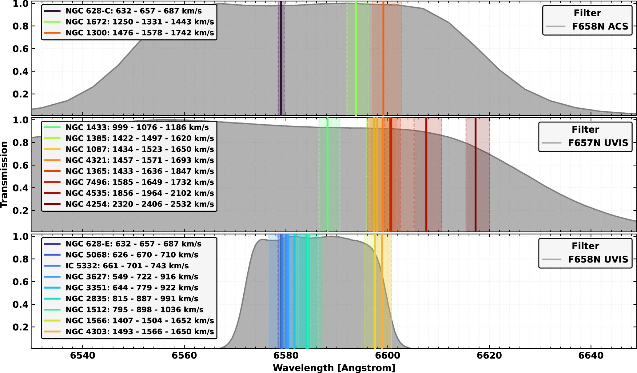
Figure 3. Filter transmission curves for the F657N (middle panel) and F658N (bottom panel) HST-Hα filters on WFC3/UVIS used in this survey. The solid vertical lines show the wavelength of the Hα line for the systemic velocity of each galaxy in our sample, while the shaded regions show the full velocity range. Observations with the narrow F658N filter are preferred, but Hα emission for galaxies with velocities higher than ≈1500 km s−1 is redshifted outside of this passband, and we use F657N instead (see Figure 10; see also Figure 16 for a comparison of HST to MUSE Hα flux as a function of velocity for two galaxies that have a velocity range close to the edge of the filter transmission curve). Archival observations for three galaxies (NGC 628-C, NGC 1300, and NGC 1672) use the F658N filter from the ACS/WFC camera (top panel).
Download figure:
Standard image High-resolution imageBoth filters have a peak throughput of 25%. We use the narrow F658N filter to observe galaxies with systemic velocities less than ≈1500 km s−1 and the F657N filter to observe those with higher velocities (note that the F657N filter was used to image NGC 1433 even though it has a velocity ≲700 km s−1).
With the WFC3/UVIS camera, we observe a single target in each visit and maximize the integration time in each exposure. A post flash of 17 or 18 e− is applied for each exposure to increase the background counts, which is recommended to mitigate issues due to charge transfer efficiency (CTE) losses. The dither sequence is optimized to cover the WFC3 chip gap. We obtain two exposures at each of two pointings using the “WFC3-UVIS-GAP-LINE” pattern, which is designed to cover the gap between the two WFC3 CCDs. The exposure times for each galaxy are listed in Column (4) of Table 2. We show footprints of the new PHANGS-HST-Hα coverage (red) and that of VLT/MUSE IFU (white) in the Appendix.
Table 2. Summary of HST Observations and MUSE Parameters
| Galaxy | Velocity | Filter Instrument | ExpTime | MUSE Res. |
|---|---|---|---|---|
| (km s−1) | (s) | (arcsec) | ||
| (1) | (2) | (3) | (4) | (5) |
| IC 5332 | 701 ± 1 | F658N WFC3 | 4 × 598 | 0.87 |
| NGC 628-C* | 657 ± 1 | F658N ACS | 2 × 711 | 0.92 |
| NGC 628-E | 657 ± 1 | F658N WFC3 | 4 × 587 | 0.92 |
| NGC 1087 | 1523 ± 2 | F657N WFC3 | 4 × 584 | 0.92 |
| NGC 1300* | 1578 ± 1 | F658N ACS | 4 × 680 | 0.89 |
| NGC 1365 | 1636 ± 1 | F657N WFC3 | 4 × 598 | 1.15 |
| NGC 1385 | 1497 ± 4 | F657N WFC3 | 4 × 550 | 0.77 |
| NGC 1433* | 1076 ± 1 | F657N WFC3 | 3 × 515 | 0.91 |
| NGC 1512 | 898 ± 3 | F658N WFC3 | 4 × 602 | 1.25 |
| NGC 1566 | 1504 ± 2 | F658N WFC3 | 4 × 632 | 0.80 |
| NGC 1672* | 1331 ± 3 | F658N ACS | 1 × 593, 3 × 617 | 0.96 |
| NGC 2835-S | 887 ± 1 | F658N WFC3 | 4 × 588 | 1.15 |
| NGC 2835-N | 887 ± 1 | F658N WFC3 | 4 × 556 | 1.15 |
| NGC 3351 | 779 ± 1 | F658N WFC3 | 4 × 586 | 1.05 |
| NGC 3627 | 722 ± 2 | F658N WFC3 | 4 × 550 | 1.05 |
| NGC 4254-E | 2406 ± 1 | F657N WFC3 | 4 × 586 | 0.89 |
| NGC 4254-W | 2406 ± 1 | F657N WFC3 | 4 × 586 | 0.89 |
| NGC 4303 | 1566 ± 2 | F658N WFC3 | 4 × 584 | 0.78 |
| NGC 4321 | 1571 ± 1 | F657N WFC3 | 4 × 587 | 1.16 |
| NGC 4535 | 1964 ± 1 | F657N WFC3 | 4 × 550 | 0.56 |
| NGC 5068-N | 670 ± 1 | F658N WFC3 | 4 × 588 | 1.04 |
| NGC 5068-S | 670 ± 1 | F658N WFC3 | 4 × 588 | 1.04 |
| NGC 7496 | 1649 ± 5 | F657N WFC3 | 4 × 608 | 0.89 |
Note. Archival observations were taken by the following programs: GO-10402 (PI: Chandar) for NGC 628-C, GO-10342 (PI: Noll) for NGC 1300, GO-13773 (PI: Chandar) for NGC 1433, and GO-10354 (PI: Jenkins) for NGC 1672. Column (5) lists the FWHM of the Gaussian PSF of the homogenized (copt) mosaic from E. Emsellem et al. (2022).
Download table as: ASCIITypeset image
Standard procedures are used to reduce and drizzle the F658N and F657N images. The exposures are processed through the Pyraf/STSDAS CALWFC3 or CALACS software, which performs initial data quality flagging, bias subtraction, gain correction, bias stripe removal, correction for CTE losses, dark current subtraction, flat-fielding, and photometric calibration and outputs “FLC” FITS files for each exposure. These files are then aligned and registered with north up and east to the left, sky subtracted, and drizzled (using the DRIZZLEPAC software package) to create a single F658N or F657N image matched to the pixel grid of the PHANGS-HST V-band images (J. C. Lee et al. 2022), with a pixel scale of 0 04. The PHANGS-HST V-band images used astrometry calibrated using Gaia DR2 sources (Gaia Collaboration et al. 2018; L. Lindegren et al. 2018). The final FITS files are in units of e− s−1, and important use cases are discussed in Section 5.
We used archival narrowband images for NGC 628-C, NGC 1300, NGC 1433, and NGC 1672. These were taken by the following programs: GO-10402 (PI: Chandar) for NGC 628-C, GO-10342 (PI: Noll) for NGC 1300, GO-13773 (PI: Chandar) for NGC 1433, and GO-10354 (PI: Jenkins) for NGC 1672. The specific filter and exposure times are compiled in Table 2 for these data as well.
As noted in the previous section, two other HST programs (besides PID 17126) continue to obtain broadband and Hα imaging of PHANGS galaxies that were not part of the PHANGS-JWST Cycle 1 Treasury sample. Specifically, PID 17457 (PI: F. Belfiore) is completing Hα imaging for the rest of the original 38 PHANGS-HST galaxies. Additionally, PID 17502 (PI: D. Thilker), a Cycle 31 Large Treasury, is obtaining both NUV-U-B-V-I and Hα for PHANGS galaxies observed by JWST in Cycle 2. When completed, these programs will expand science analysis such as described herein to 74 galaxies, each with HST+JWST+ALMA data sets. The PHANGS collaboration is working to obtain MUSE IFU spectroscopy for as many of these as possible.
3.2. MUSE Observations
The PHANGS-MUSE survey has carried out observations with the MUSE integral field spectrograph at the ESO VLT to map the 19 nearby spiral galaxies that form our sample (E. Emsellem et al. 2022). The footprints of the PHANGS-MUSE survey were designed to maximize overlap with the PHANGS-ALMA CO (2–1) maps and are shown in the Appendix (Figure 15). The spatial resolutions of the MUSE observations for each galaxy are compiled in Table 2. PHANGS-MUSE has produced ≈15 × 106 spectra that have a wavelength coverage of 4800–9300 Å with a spectral resolution going from ∼80 km s−1 at the blue end to ∼35 km s−1 at the red end and targeting key optical lines, including Hβ, [O iii] λ5006, [O i] λ6300 [S ii] λλ6716, 6731, Hα, and [N ii] λ6583.
The data reduction process is described in detail in E. Emsellem et al. (2022). The data cubes are publicly available from the ESO archive.32 In this work, we use the PHANGS-MUSE spectra to help anchor the flux calibration of our HST-Hα images and to correct for [N ii] contamination, as described in Section 4.
4. Processing of PHANGS-HST-Hα Images
In this section, we describe our PyHSTHAContSub33 pipeline for producing flux-calibrated, continuum-subtracted high-resolution HST-Hα maps (see flowchart in Figure 4). There are a number of challenges in determining and correcting for the background level (which is not well constrained for the HST images) and correcting for contamination from [N ii] line emission that is included in the passband. For these purposes, we leverage our MUSE/IFU spectroscopy (E. Emsellem et al. 2022), which provides direct constraints on the [N ii] contamination (convolved with the HST filter transmission) and has been calibrated to correctly match the background level. Post-processing steps correct for remaining artifacts, including cosmic-ray residuals, foreground stars, and strongly negative regions where the continuum has been oversubtracted.
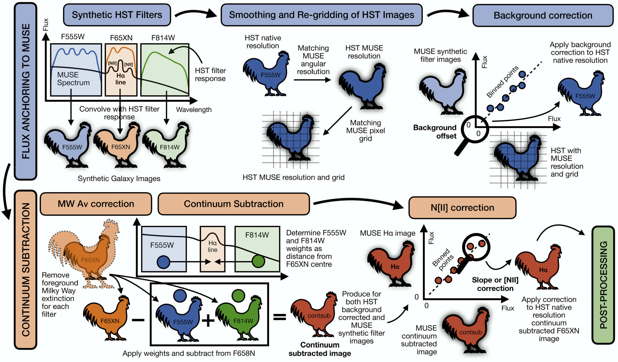
Figure 4. Overview of the PyHSTHAContSub (doi:10.5281/zenodo.14610187) pipeline background and continuum subtraction steps used to produce the HST-Hα images (see Section 4). In our workflow, we first generate synthetic HST filter images from the MUSE data (Section 4.1). We then smooth and regrid the HST images (while preserving flux) to the resolution and pixel grid of the synthetic MUSE images. We compare these images and determine a background correction, which we apply to the full-resolution HST images. For the continuum subtraction, we first subtract the Milky Way foreground extinction from each filter (for both the MUSE and HST data). We then determine the weights of the two broadband images and subtract a combination of these two from the narrowband image to produce the continuum-subtracted narrowband images. We do this for both the HST and MUSE observations. We then compare the MUSE Hα image with the continuum-subtracted MUSE image to determine the contribution of [N ii] line emission in the narrowband filter, which we then apply to the full-resolution HST images. These final images are then passed to the post-processing steps to correct for oversubtraction, remaining cosmic-ray, and foreground-star residuals. Here the chickens represent the individual galaxy images.
Download figure:
Standard image High-resolution image4.1. Synthetic MUSE Images
We generate synthetic images from the MUSE data cubes integrating over the HST F657N, F658N, F555W, and F814W filters associated with the appropriate camera+ filter (WFC3/UVIS or Advanced Camera for Surveys (ACS)/WFC) for each galaxy (see Appendix A.3 for comparison of alternative filter selection).
The wavelength coverage of the MUSE spectra does not fully cover the range of the F555W and F814W transmission curves (see Figure 5). Consequently, a small fraction of the emission remains unaccounted for in the synthetic images. However, the continuum subtraction is performed in units of flux density (rather than flux; see below), so the small missing bandwidth does not significantly affect the final HST-Hα maps.
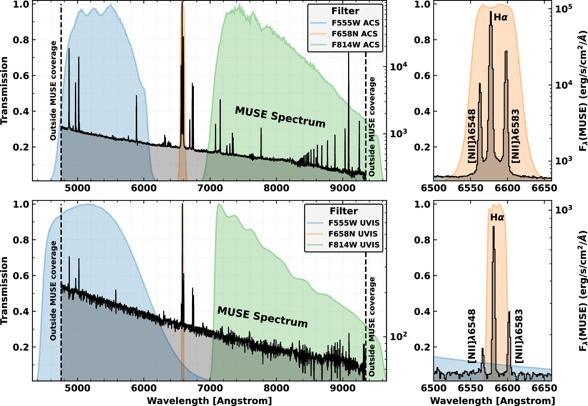
Figure 5. Example MUSE spectra compared with HST filter transmission curves (ACS/WFC and WFC3/UVIS). Example spectra from NGC 628 (top panel) and NGC 2835 (bottom panel) are shown as solid black lines, overlaid with the F555W (blue), F658N (orange), and F814W (green) filter transmission curves for ACS/WFC (top panel) and WFC3/UVIS (bottom panel). The left panel displays the full wavelength range of the MUSE observations, with dashed vertical lines marking the coverage limits. In the right panel, we focus on the Hα line within the F658N filter bandpass, which includes contributions from the [N ii] λ6548 and [N ii] λ6583 emission lines.
Download figure:
Standard image High-resolution image4.2. Convert Images to Flux Density
The HST and synthetic MUSE images are all converted to the same units of flux density (erg s−1 cm−2 Å−1 pixel−1). To convert the HST images from units of electrons s−1 to flux density, we employ the photflam parameter. The photflam value is for a source with a constant flux per unit wavelength in units of erg s−1 cm−2 Å−1 that produces a count rate of 1 count s−1 and is taken from the header of the HST images. Additionally, we use the SYNPHOT package34 to calculate photplam, or the pivot wavelength (“pivot” parameter), and photbw, or the width of the filter (“rectwidth” parameter). These parameters for all filters are summarized in Table 3.
Table 3. Parameters Taken from synphot.SpectralElement
| Instrument | Filter | Photflam | Photplam | Photbw |
|---|---|---|---|---|
| (×10−19 cm2 Å s erg−1) | (Å) | (Å) | ||
| ACS/WFC | F555W | 1.988 | 5361.0 | 1124.6 |
| ACS/WFC | F658N | 20.063 | 6584.0 | 74.9 |
| ACS/WFC | F814W | 0.712 | 8045.5 | 1741.5 |
| WFC3/UVIS | F555W | 1.827 | 5308.4 | 1565.4 |
| WFC3/UVIS | F657N | 21.814 | 6566.6 | 121.0 |
| WFC3/UVIS | F658N | 97.583 | 6585.6 | 27.5 |
| WFC3/UVIS | F814W | 1.499 | 8039.0 | 1565.2 |
Note. These are used to convert the filter images from units of counts s−1 to units of flux density (Section 4.2) and the Hα images into flux (Section 4.5).
Download table as: ASCIITypeset image
4.3. Match HST Images to MUSE Resolution
Next, we smooth and regrid the HST images to match the resolution and pixel grid of the synthetic MUSE images (see Figure 6).
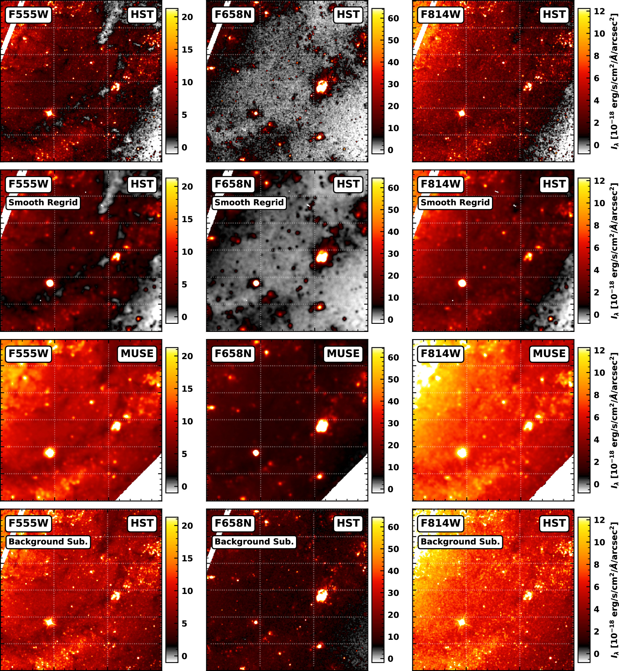
Figure 6. HST and MUSE Filters for NGC 628. First row, left to right: HST F555W, F658N, and F814W filters at their native resolution (∼0 1) and pixel grid. Second row, left to right: HST filters smoothed to the resolution and grid size matching the MUSE observations (see next row of panels). Third row, left to right: synthetic images produced by applying the HST transmission curves to the lower-resolution MUSE spectroscopic observations. These are used to improve the flux calibration of the HST images. Fourth row, left to right: HST filter maps (again at native resolution and pixel grid) with zero-point offsets applied; offsets determined by comparing with the synthetic MUSE images (see Figure 7).
Download figure:
Standard image High-resolution imageWe first smooth all HST images using a Gaussian function with a size of

where the resolutions of the MUSE observations (θMUSE) for each galaxy are compiled in Table 1 (see E. Emsellem et al. 2022) and the HST resolution (θHST) is assumed to be 0 1. In practice, the point-spread function (PSF) of the HST observations is not necessarily a Gaussian (J. E. Krist et al. 2011) and will fluctuate by ≈0
 02 around this value depending on the filter and pixel coordinates. However, since the HST images have a spatial resolution approximately an order of magnitude higher than the MUSE observations and are, hence, smoothed significantly during this step of the procedure, small variations in the PSF/shape of the beam of the HST images have essentially no impact on the resulting MUSE-resolution-matched HST-Hα maps.
We convolve the smoothed HST images to the same pixel grid as the synthetic MUSE images (pixel size of 0 2) using a bilinear function (making use of the astropy.convolution.convolve_fft function; Astropy Collaboration et al. 2018).
4.4. Background Level from MUSE Observations
We compare the flux density values in each pixel of the matched-resolution HST and synthetic MUSE images. The best linear fit between these will be used to anchor fluxes in the HST images to the more accurate MUSE values. To determine this relation, we first mask pixels that (1) are contaminated by bright foreground stars (identified from MUSE; B. Groves et al. 2023) and (2) limit the data to a range around zero. The latter was done since in this step we are primarily interested in the calibration of any zero-point offset between the two images and therefore want to limit the dependence of our fitting on the bright emission regions. We limit the data between the 0.01th and 99th percentiles in the HST and synthetic MUSE images. In addition, we bin the flux data into 25 bins, which again limits the impact of outlier pixels on the fit. A similar method was recently employed for the calibration of the PHANGS-JWST images (A. K. Leroy et al. 2023; T. G. Williams et al. 2024). Lastly, a linear least-squares fitting (y = ax + b, where y represents the HST image data points and x represents the MUSE image data points) was performed.
The results of this analysis can be seen in Figure 7, which shows the matched-resolution HST (y-axis) and synthetic MUSE (x-axis) flux densities for the F555W, F658N, and F814W filters toward NGC 628-C, as well as the binning and fitting routines. We apply the background correction from these solutions to the full-resolution HST images as ybgsub = y − b (i.e., we do not correct for the slope of the fit, but only the background offset).35 The background correction offsets for each galaxy and each filter are given in Table 4.
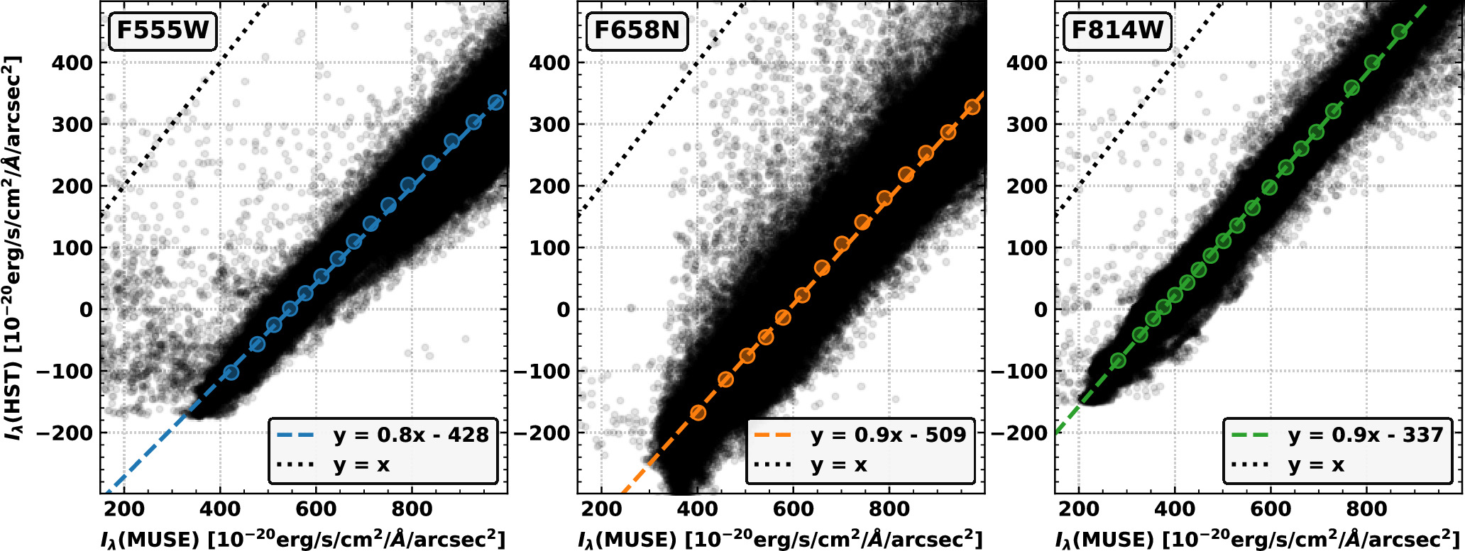
Figure 7. Fits to determine the background level in HST images by calibrating to MUSE observations (Section 4.4). Intensities from matched-resolution pixels in the HST vs. synthetic MUSE images measured in the F555W, F658N, and F814W filters for NGC 628-C. The colored circles represent 25 binned data points (spaced by data density), and the dashed line in each panel shows the best linear fit to these points (y = ax + b), where y represents measurements from the degraded HST pixels and x represents the MUSE pixels (see Table 4). The dotted line in each panel shows the 1-to-1 line. The best-fit offsets are subtracted from the full-resolution HST images to correct for the sky background level.
Download figure:
Standard image High-resolution imageTable 4. Results of Fitting for the Background Correction in Each of the HST Filters (Section 4.4), and the Correction Factor for the [N II] λλ6548, 6583 Line Contamination in the Hα Images (Section 4.6)
| Galaxy | Background Corrections | [N ii] Correction | ||
|---|---|---|---|---|
| (erg s−1 cm−2 Å−1 arcsec−2) | ||||
| F555W | F65XN | F814W | Factor | |
| IC 5332 | −290.78 | 1801.13 | −190.29 | 1.11 |
| NGC 628-C | −428.03 | −509.67 | −337.13 | 1.35 |
| NGC 628-E | −123.81 | 1637.38 | −196.70 | 1.19 |
| NGC 1087 | −217.99 | 886.88 | −147.06 | 1.18 |
| NGC 1300 | −84.71 | −92.37 | −51.87 | 1.26 |
| NGC 1365 | −777.32 | 520.94 | −687.02 | 1.25 |
| NGC 1385 | −242.34 | 890.50 | −164.83 | 1.21 |
| NGC 1433 | −617.62 | −620.56 | −534.81 | 1.33 |
| NGC 1512 | −161.94 | 1414.89 | −140.05 | 1.03 |
| NGC 1566 | −1030.71 | 1660.55 | −575.82 | 1.03 |
| NGC 1672 | −194.30 | −348.71 | −163.62 | 1.38 |
| NGC 2835-S | −465.89 | 751.65 | −342.54 | 1.02 |
| NGC 3351 | −180.02 | 542.77 | −164.60 | 1.07 |
| NGC 3627 | −764.28 | 10.71 | −672.63 | 1.16 |
| NGC 4254 | −87.41 | 120.74 | −205.08 | 0.94 |
| NGC 4303 | −1153.58 | −386.42 | −848.63 | 0.97 |
| NGC 4321 | −804.18 | 668.72 | −667.56 | 1.23 |
| NGC 4535 | −610.03 | 672.52 | −487.48 | 1.11 |
| NGC 5068 | −247.92 | −55.93 | −157.27 | 1.10 |
| NGC 7496 | −201.02 | 506.70 | −146.29 | 1.22 |
Download table as: ASCIITypeset image
This procedure yields HST-Hα maps with a robust background level anchored to match the MUSE measurements.
4.5. Continuum Subtraction
The purpose of this step is to subtract the stellar continuum present in the narrowband HST filter images (see Figure 5). To achieve this, we utilize the HST F555W and F814W images, which are dominated by the stellar continuum and have been flux anchored to the synthetic MUSE images, as described in the previous section. We note that our procedure would also work with other filters. For example, the F550M or F547M filter could replace the F555W filter, as demonstrated in the Appendix.
We begin by correcting the observations for foreground extinction due to the Milky Way. This is achieved using the extinction law of J. A. Cardelli et al. (1989) and E(B − V) values from E. F. Schlafly & D. P. Finkbeiner (2011). Although this adjustment results in a relatively minor flux correction (on the order of 10%), it is important for accurate continuum subtraction. Without it, systematic over- or undersubtraction could occur across filters owing to the wavelength dependence of extinction. Additionally, the same foreground extinction correction has been applied to the MUSE DAP Hα maps, which are used to account for the contribution of the [N ii] line, as detailed in E. Emsellem et al. (2022).
To estimate the continuum flux in the narrowband F658N or F657N filter, we calculate weighting factors, W, based on the relative differences in the central wavelengths of the broad- and narrowband filters:


where λF555W, λF814W, and λF65XN are the central “pivot” wavelengths of the F555W, F814W, and either F657N or F658N filters, respectively, determined from their respective transmission filter response curves (see Section 4.2). The continuum image is produced in logarithmic space as

where FF555W and FF814W are the pixel fluxes in the F555W and F814W images (in units of erg cm−2 s−1 Å−1). The continuum-subtracted Hα image is then produced in linear space as

where FF65XN represents the pixel fluxes in either the F657N or F658N image. As a final step, we convert the continuum-subtracted images from units of flux density to units of flux using the filter bandwidth (from the respective transmission filter response curve; see Section 4.2).
The result of this continuum subtraction routine can be seen in Figure 8. Here the bright nebulae are cleanly separated from the background stellar continuum across the whole disk of the galaxy (in this case NGC 628). There are, however, low-level artifacts that are difficult to remove, e.g., due to diffuse stellar emission toward the center of the galaxy or compact stellar clusters that may have continuum spectra that are not well recovered by only using the (log) interpolation of the two broadband observations. It is also worth noting that artifacts in either of the broadband or narrowband images become more prominent in the continuum-subtracted image, due to the relative intensity of the nebula emission to stellar emission.
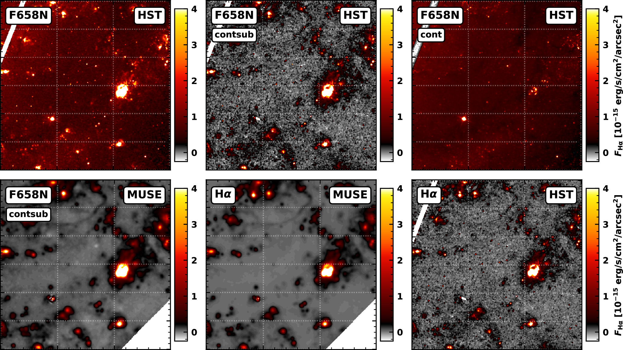
Figure 8. Results of the extinction correction, continuum subtraction (Section 4.5), and [N ii] correction (Section 4.6) of a portion of NGC 628-C (same as Figure 6). Top row, from left to right: shown is the F658N filter image after background subtraction and extinction correction, and the continuum-subtracted and continuum F658N filter images. Bottom row, from left to right: the continuum-subtracted F658N image produced from the synthetic HST filter MUSE images (i.e., including the contribution from the [N ii] lines convolved with the F658N filter transmission curve), the MUSE DAP Hα-emission-only image (E. Emsellem et al. 2022), and the final [N ii]-corrected HST-Hα image.
Download figure:
Standard image High-resolution image4.6. Correction for [N ii] Emission
The final global correction applied to the HST-Hα images accounts for the contribution from the [N ii] λ6548 and [N ii] λ6583 lines, which can fall within the narrowband F658N and F657N filters depending on the HST filter and the velocity of the galaxies (see Figure 5). For this correction, we compare the HST-filtered MUSE images36 with the DAP Hα image to determine the correction factor. This factor is subsequently applied to the full-resolution continuum-subtracted HST observations. Using the MUSE data alone to derive this correction factor, rather than employing the smoothed HST observations, was motivated by the goal of conducting a consistent test using data from the same set of observations.
To do so, we conduct the continuum subtraction analysis (including the MW extinction correction) outlined in Section 4.6 using the broadband and narrowband synthetic MUSE images for each galaxy. This produces MUSE continuum-subtracted emission maps, with the Hα and [N ii] lines convolved with the filter transmission curves for each galaxy (see maps in bottom panels of Figure 8).37
Next, we compare the MUSE continuum-subtracted emission maps and the MUSE DAP Hα emission-line maps (see Figure 9). We mask the outlying pixels with percentiles in both the MUSE continuum-subtracted and DAP Hα maps (1%−99% in this case), bin the remaining points into 20 equally spaced bins, and perform a least-squares fit to the binned data points assuming a linear polynomial (y = ax + b, where y represents the MUSE continuum-subtracted emission data points and x represents the MUSE DAP Hα emission-line data points; as shown in Figure 9). We then divide the full-resolution HST fluxes by this factor (a), to obtain the HST-Hα-only emission-line maps.38
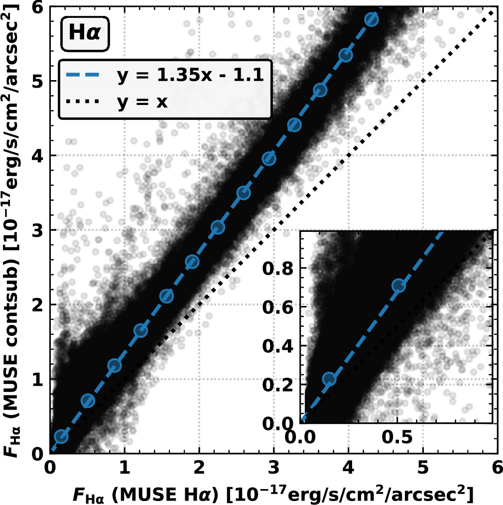
Figure 9. Results of the [N ii] λ6548 and [N ii] λ6583 line correction routine (Section 4.6). Hα fluxes are from the continuum-subtracted MUSE synthetic filter maps as a function of the Hα flux densities measured from the MUSE spectroscopic data. The blue circles represent 20 binned data points (equally spaced), and the dashed blue line shows the best linear fit to these points (y = ax + b), where y represents the HST image data points and x represents the MUSE data points (see Table 4). The dotted line shows the 1-to-1 line.
Download figure:
Standard image High-resolution imageIt is worth noting that the relative contribution of these lines is somewhat challenging to constrain on a pixel-by-pixel basis across all galaxies. The exact contribution depends on the velocity, how the lines fall within the HST filter transmission curves, and the intrinsic nature and morphology of the specific source. For instance, assuming a global correction factor could introduce systematic errors in the flux with galactocentric radius, particularly in galaxies with strong metallicity gradients. In such cases, this approach might result in subtracting too little flux near the center and too much flux near the edges. Indeed, we find that NGC 4303 has a correction factor slightly below 1, which in principal should not be possible. This may be attributed to this issue, although this galaxy does not exhibit a particularly strong metallicity gradient (see B. Groves et al. 2023). This discrepancy could also arise from imperfect continuum subtraction and/or absorption of the Hα (which is corrected for in the MUSE DAP fits; see E. Emsellem et al. 2022).
Figure 9 shows an example of this procedure for one galaxy, NGC 628, where we find a [N ii] correction factor of 1.35. The final correction factors determined individually for each galaxy are compiled in Table 4. Again, we note that fixing the intercept of the fits to zero makes only a minor change to the correction factors (see Table 6 in the Appendix).
We conduct a number of consistency checks of the resulting images. To do so, we sum the fluxes in the final HST-Hα and MUSE Hα maps within the masks from the MUSE nebula catalogs. In Figure 10, we plot the histogram distributions of this flux ratio for all sources within the catalog. We see that the ratios scatter around 1, which highlights that the correction of the [N ii] contribution in the HST data is reasonable. We note that we do not use the HST data to estimate this correction factor, but rather the synthetic MUSE observations, and despite this, the correlations are close to unity. We fit a Gaussian to the distribution for all galaxies and see that they have a standard deviation of around 30%. Limiting the fit to the brightest regions above 10−15 erg s−1 cm−2, we see that this deviation decreases to around 15%. We use these as the uncertainty confidence limits on our flux measurements across the HST-Hα images.
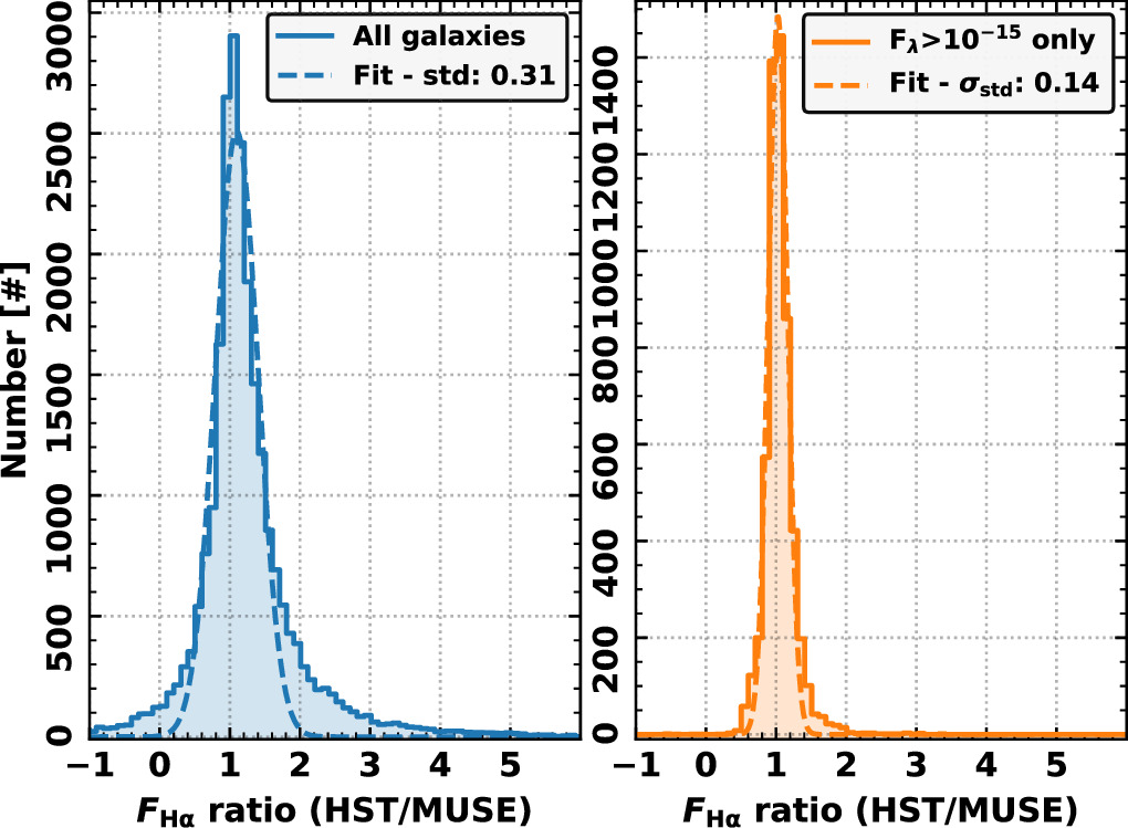
Figure 10. Histograms of the final HST-to-MUSE Hα flux ratios. We show histograms of the HST-to-MUSE Hα flux ratios for all regions (left panel) and for regions with MUSE Hα fluxes higher than 10−15 erg s cm−2 (right). The dashed curves show the best-fit Gaussian distribution in each panel, and the 1σ standard deviation is written in the upper right corner. For the bright Hα regions, ≈70% of the pixels in the HST-Hα maps have fluxes within just ≈15% of those measured from the MUSE spectra.
Download figure:
Standard image High-resolution imageIn Figure 11, we plot the ratio of these fluxes as a function of the MUSE Hα, MUSE Hα velocity, galactocentric radius, and MUSE Hα equivalent width. Across the sample, we see evidence for mild systematic trends with galactocentric radius or velocity in a few cases, likely due to the emission shifting out of the filter (see Figure 16).
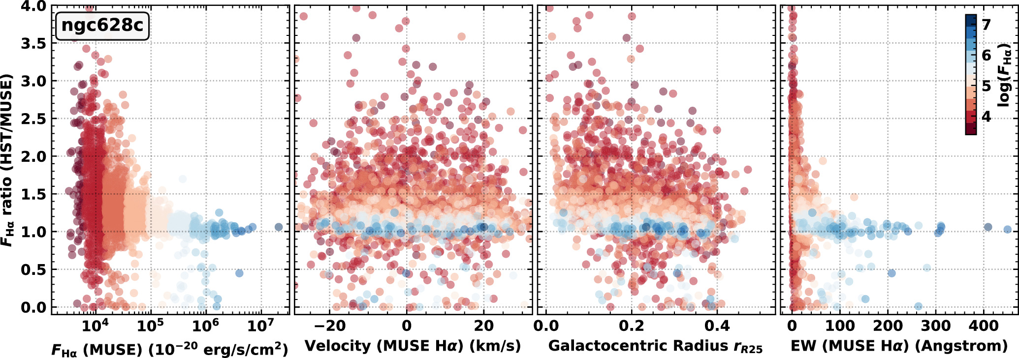
Figure 11. The ratio of HST to MUSE Hα fluxes in NGC 628-C is checked against other nebula properties. We show (from left to right) the Hα flux ratio vs. the MUSE Hα flux (left panel), MUSE Hα velocity (second panel), galactocentric radius (third panel), and the Hα equivalent width measured directly from the MUSE spectra (right panel). There is no obvious trend in the flux ratio with Hα velocity or galactocentric distance (middle two panels).
Download figure:
Standard image High-resolution image4.7. Error Maps
To produce HST-Hα error maps, we use the inverse variance (1/V) images for the individual filters (see J. C. Lee et al. 2022). These maps incorporate contributions from the detector and the Poisson noise toward the target, modulated by the number of integrations drizzling into an output pixel and the effective exposure depth after masking, respectively. We convert the inverse variance image into a map of the uncertainties in units of counts s−1 (i.e.,  ) and then into flux density (erg cm−2 s−1 Å−1 arcsec−2; see Section 4.2). To produce errors for the continuum-subtracted narrowband images, we propagate the individual pixel errors in all the bands as




and then carry this forward to the continuum-subtracted flux density as

This is converted into units of flux (see Section 4.5) and corrected by the [N ii] factor (see Section 4.6). We note that these error maps do not account for uncertainties in the zero-point offset or in the [N ii] correction factor but are scaled accordingly by the correction factor such that they are representative of the errors in the final Hα images. In Table 5 we provide some statistics of the noise across the HST-Hα error maps.
Table 5. Noise Statistics of the Continuum-subtracted Hα Images and Associated Error Maps for Each Galaxy
| Galaxy | Map Properties | Error Map Properties | ||||||||||||
|---|---|---|---|---|---|---|---|---|---|---|---|---|---|---|
| (×10−17 erg s−1 cm−2 arcsec−2) | (10−17 erg s−1 cm−2 arcsec−2) | |||||||||||||
| Mean | Median | 5% | 16% | 84% | 95% | σSTD | Mean | Median | 5% | 16% | 84% | 95% | σSTD | |
| IC 5332 | 6.5 | 4.0 | −92.4 | −54.1 | 64.6 | 108.0 | 59.3 | 77.9 | 73.4 | 66.5 | 69.1 | 80.4 | 93.2 | 4.9 |
| NGC 0628-C | 15.4 | 8.9 | −31.4 | −15.4 | 36.8 | 64.1 | 25.6 | 43.3 | 41.4 | 36.7 | 38.5 | 46.2 | 55.1 | 3.4 |
| NGC 0628-E | 5.9 | 3.3 | −99.3 | −58.3 | 67.6 | 114.7 | 62.8 | 82.1 | 77.2 | 69.9 | 72.7 | 85.0 | 101.4 | 5.2 |
| NGC 1087 | 18.4 | 9.9 | −92.0 | −51.8 | 77.8 | 136.1 | 64.1 | 82.1 | 75.4 | 67.0 | 69.9 | 85.5 | 99.5 | 6.7 |
| NGC 1300 | 4.0 | 2.4 | −22.5 | −12.5 | 18.2 | 30.7 | 15.2 | 27.6 | 26.4 | 23.6 | 24.7 | 29.0 | 34.0 | 2.0 |
| NGC 1365-N | 29.9 | 13.9 | −79.6 | −42.4 | 76.4 | 135.1 | 58.6 | 75.0 | 68.8 | 60.9 | 63.6 | 79.6 | 95.7 | 6.5 |
| NGC 1385 | 18.6 | 8.0 | −93.7 | −53.4 | 76.0 | 138.4 | 63.9 | 80.3 | 74.1 | 65.8 | 68.8 | 84.8 | 100.8 | 6.5 |
| NGC 1433 | 14.0 | 3.9 | −92.4 | −53.8 | 64.7 | 110.5 | 59.1 | 82.1 | 75.7 | 66.6 | 70.0 | 86.3 | 102.8 | 7.0 |
| NGC 1512 | 5.3 | 2.3 | −102.5 | −60.3 | 67.3 | 114.5 | 63.7 | 84.8 | 77.1 | 69.1 | 72.1 | 85.9 | 102.1 | 5.8 |
| NGC 1566 | 26.7 | 11.3 | −91.1 | −50.5 | 80.4 | 145.1 | 64.6 | 81.7 | 75.0 | 67.0 | 69.9 | 84.2 | 99.5 | 6.1 |
| NGC 1672 | 21.3 | 6.4 | −29.8 | −15.2 | 31.9 | 62.3 | 22.8 | 37.2 | 36.8 | 27.2 | 29.4 | 41.7 | 48.9 | 5.7 |
| NGC 2835-S | 12.9 | 7.8 | −118.1 | −67.7 | 87.7 | 148.0 | 77.4 | 99.8 | 93.3 | 84.0 | 87.6 | 102.3 | 120.9 | 6.4 |
| NGC 3351 | 14.5 | 3.9 | −103.0 | −60.1 | 71.0 | 121.2 | 65.3 | 86.5 | 79.9 | 71.7 | 74.7 | 90.0 | 105.7 | 6.3 |
| NGC 3627 | 39.3 | 24.8 | −86.4 | −42.6 | 103.2 | 186.3 | 71.4 | 86.1 | 81.6 | 72.7 | 75.9 | 92.6 | 109.0 | 7.1 |
| NGC 4254 | 29.2 | 19.7 | −112.0 | −60.0 | 108.5 | 186.2 | 83.2 | 101.3 | 95.5 | 81.6 | 87.8 | 109.0 | 128.7 | 9.2 |
| NGC 4303 | 38.2 | 21.1 | −101.2 | −52.5 | 105.2 | 188.3 | 77.4 | 94.2 | 87.6 | 77.8 | 81.4 | 98.1 | 115.6 | 7.3 |
| NGC 4321 | 20.5 | 12.7 | −86.4 | −46.8 | 77.6 | 134.2 | 61.6 | 77.5 | 72.3 | 64.1 | 67.1 | 80.9 | 97.4 | 5.9 |
| NGC 4535 | 19.5 | 12.5 | −98.8 | −54.6 | 82.7 | 134.6 | 68.5 | 90.5 | 84.9 | 76.0 | 79.3 | 93.9 | 108.3 | 6.6 |
| NGC 5068 | 19.5 | 13.5 | −103.2 | −56.2 | 88.0 | 147.2 | 71.5 | 90.5 | 88.2 | 62.5 | 80.3 | 96.9 | 112.1 | 7.2 |
| NGC 7496 | 14.5 | 5.8 | −81.5 | −46.6 | 61.3 | 104.0 | 53.8 | 71.1 | 65.6 | 57.9 | 60.7 | 73.5 | 87.2 | 5.6 |
Note. Compiled are the mean and pixel values at 50th (median), 5th, 16th (−σ), 84th (+σ), and 95th percentiles, as well as (median absolute) standard deviation for each map (σSTD).
Download table as: ASCIITypeset image
4.8. Post-processing
As the final part of our data reduction pipeline, we post-process the images to remove remaining artifacts such as cosmic-ray residuals, strong negative features caused by oversubtraction of the continuum level, and foreground stars. These post-processing steps provide an optimal “artifact free” image set, although some biases may be introduced in the noise.
4.8.1. Cosmic-Ray Correction
After the main image processing steps, a number of bright cosmic-ray residuals not associated with any emission-line source remain in the HST-Hα images. These are particularly noticeable in the archival data sets that have fewer exposures and hence have less effective cosmic-ray removal during the image reduction process (e.g., NGC 628).
To remove these contaminants, we apply the Deep Learning Based Cosmic Ray Removal for Astronomical Images (deepCR) package (K. Zhang & J. S. Bloom 2020) with the ACS-WFC-F606W.pth learned model to generate a probability map of cosmic-ray residuals. We apply a conservative 0.9 probability threshold for galaxies observed as part of our PHANGS-HST-Hα Treasury survey (GO-17126) and a less restrictive 0.25 threshold for the archival images. Masked pixel values are interpolated and replaced using the astropy.convolution.interpolate_replace_nans function.39
4.8.2. Continuum Oversubtraction
In a number of cases, strong continuum sourcesm, including bright clusters, foreground stars, and even chance supernovae (e.g., the case of SN 2020oi in NGC 4321), are oversubtracted and result in negative values in the flux-calibrated, continuum-subtracted HST-Hα images. To identify and mitigate these regions on the maps, we create two masks with the locations of negative pixels: a “strong” negative mask that includes pixels with values <−5σrms, and another with a lower threshold of <−σrms. We grow the strong negative mask into the lower threshold mask and replace values within this final mask with an interpolated value from the astropy.convolution.interpolate_replace_nans function.
4.8.3. Foreground Star Removal
There are a number of bright, saturated foreground stars that are very evident and produce clear artifacts in our HST-Hα images. To remove these features, we use previously defined star masks created for the MUSE data set (B. Groves et al. 2023). These are based on Gaia objects within the MUSE field of view and then differentiated between stars and clusters (galaxy centers are often included) by the presence of the calcium triplet and/or abnormal fits. In addition to these, we manually inspected all of the background-subtracted images and produced an additional catalog of bright foreground stars that result in artifacts. We then substitute regions from both these catalogs with noise profiles that mimic the image as a whole.
4.8.4. Mosaic Image for NGC 628
NGC 628 was observed using both the WFC3/UVIS (NGC 628-E) and ACS/WFC (NGC 628-C) instruments (see Table 2). Because these data sets require separate calibration steps (due to differences in filter response and noise properties), we did not merge them into a single mosaic at the initial narrowband data processing stage. Instead, both images were fully processed individually (i.e., background subtraction, extinction correction, and continuum subtraction), to produce separate continuum-subtracted Hα images. With these Hα images (and their corresponding error maps) now in equivalent flux units, we combined them into one final Hα mosaic. NGC 628 is the only case in our 19-galaxy sample where this post-processing combination step is required.
5. Hα Nebula Catalogs and Scientific Applications
5.1. Final Hα Images
HST-Hα emission, seen as the pinkish-red emission in Figure 1, shows the variety of star-forming environments encompassed by the PHANGS-HST-Hα sample. There are several galaxies with compact star-forming rings (including NGC 1512, NGC 1672, and NGC 4321). A number of the spirals in our sample have nuclear star formation, with clumpy Hα associated with nuclear star-forming regions (e.g., NGC 1385, NGC 5068, and NGC 7496). In the barred galaxies (e.g., NGC 1512, NGC 1672, NGC 3627, NGC 7496) it is very obvious that star formation does not occur in the bar, but rather in the center and at the ends of the bar (e.g., A. Fraser-McKelvie et al. 2020). Our sample also includes galaxies with flocculent and grand-design spiral arms. In some galaxies, weak interarm Hα emission is observed, where weak star formation is taking place (e.g., NGC 4254).
The new maps also show a wide range of source morphologies on smaller scales. There are many individual compact and unresolved H ii regions, as well as large complex ones. There are superbubbles (A. T. Barnes et al. 2023; E. J. Watkins et al. 2023) and partial shells with a range of sizes, as well as diffuse Hα emission.
5.2. Data Products
The flux-calibrated emission-line PHANGS-HST-Hα maps will support a number of science projects. The current data release includes the reduced drizzled images and the flux-calibrated, continuum-subtracted Hα maps (more below), which are available via MAST,40 as well as at the Canadian Astronomy Data Centre as part of the PHANGS archive.41
- 1.We release reduced, drizzled images in units of flux density, which have been aligned and drizzled onto the same pixel grid as the five broadband PHANGS-HST images from J. C. Lee et al. (2022). These images include both line and stellar continuum emission and are ideal for including in spectral energy distribution (SED) fitting to determine the age and reddening of star clusters (see Section 5.3). For these, we will release the DRC FITS images of the individual pointings and mosaicked DRC FITS images for the galaxies that have multiple pointings.
- 2.We also release the flux-calibrated, continuum-subtracted Hα maps in units of erg s−1 cm−1 arcsec−2, which were created as described in Sections 4.1−4.7; images that have gone through the additional post-processing steps are available upon request. These images are ideal for identifying individual H ii regions, even very small and faint ones that are not detected in the ground-based MUSE/IFU observations (Section 3.2). They also provide a unique opportunity to measure the radii of H ii regions (Section 5.5), which is quite challenging from the ground and will lead to significantly improved calculations of key stellar feedback processes such as internal pressure from radiation, thermal gas, and winds. These images also reveal diffuse ionizing gas in spiral galaxies, including the warm ionized gas leaking out of H ii regions (Section 5.6).
5.3. Improving Cluster Age, Reddening, and Mass Estimates by Including Hα
Age and mass are two of the most basic properties of a star cluster. Accurate determinations of the ages and masses of clusters are critical to address many fundamental questions related to stellar feedback and star and cluster formation and evolution. However, low-metallicity, dust-free ancient clusters are difficult to distinguish from young, dust-rich clusters or from intermediate-age moderately dusty clusters when only broadband optical observations are used. Breaking this age–reddening–metallicity degeneracy is sufficiently challenging that ≈80% of likely ancient globular clusters were incorrectly dated using five broadband filters to ages ≲100 Myr by the original PHANGS-HST pipeline (e.g., J. A. Turner et al. 2021; B. C. Whitmore et al. 2023; M. Floyd et al. 2024), and a significant fraction of intermediate-age (≈20–500 Myr) clusters were best fit by an extremely young age of 1 Myr and moderate to high reddening (e.g., D. Thilker et al. 2025, in preparation; K. Henny et al. 2025, in preparation).
Knowing whether Hα line emission is present or absent can significantly improve cluster age estimates (e.g., R. Chandar et al. 2016; G. Ashworth et al. 2017; B. C. Whitmore et al. 2023). While including a short-wavelength broadband filter (such as in the NUV and/or U band) is important, the line emission measured in a narrowband filter, like the F658N or F657N filters used in this program, is one of the most direct ways to distinguish very young (≲6 Myr), gas-rich clusters from older, gas-free clusters. Figure 12 shows median SEDs for samples of very young, gas- and dust-rich clusters (shown in blue) and for ancient, dust-free clusters (shown in red) in 10 PHANGS-HST-Hα galaxies (K. Henny et al. 2025, in preparation). While dust-rich young and dust-free old clusters can have red broadband optical colors (decreasing flux density at shorter wavelengths), the young clusters have strong Hα line emission that clearly distinguishes them from the older clusters. Improved age, reddening, and mass estimates from SED fitting that includes Hα photometry from the images presented here will be presented in D. Thilker et al. (2025, in preparation) and K. Henny et al. (2025, in preparation).
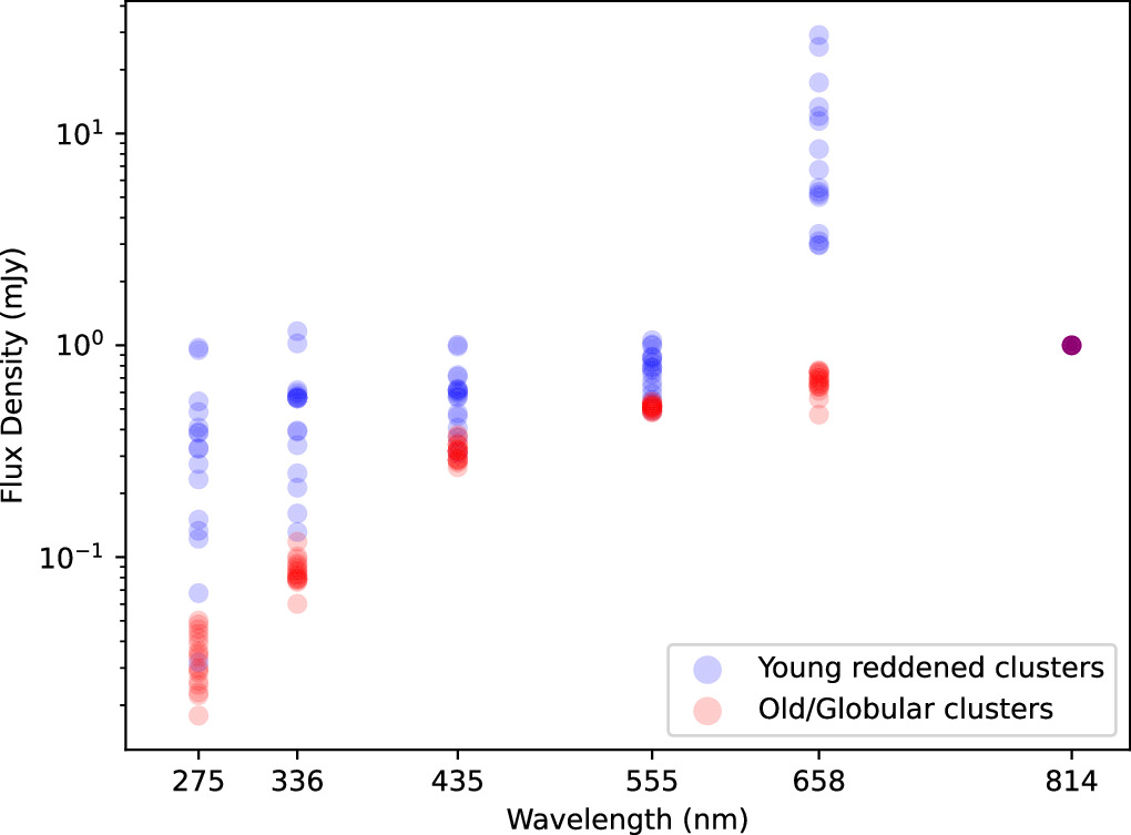
Figure 12. Median HST-based SEDs of young, gas- and dust-rich clusters (blue points) and old globular clusters (red points) for 10 PHANGS-HST-Hα galaxies. The SEDs are normalized at the I band. The young and old populations can have similar declining broadband fluxes toward shorter wavelengths but have very different Hα fluxes (see the clear separation between red and blue data points at 658 nm). Figure adapted from K. Henny et al. (2025, in preparation).
Download figure:
Standard image High-resolution imageFor some clusters with no Hα emission, it can still be challenging to separate those with ages ≈7–10 Myr and moderate reddening from somewhat older (≈20–50 Myr) clusters with little reddening. In these cases, the presence or absence of near-infrared emission from red supergiants with ages ≈7–10 Myr in NIRCAM photometry further improves age-dating (K. Henny et al. 2025, in preparation).
5.4. New Catalog of Ionized Gas Nebulae
Warm ionized gas in spiral galaxies originates from H ii regions, supernovae/SNRs, and PNe. Ultraviolet photons can escape from these nebulae and ionize gas far from their birth sites, giving rise to DIG. Identifying nebulae, particularly compact ones, and separating them from DIG in nearby galaxies can be challenging in imaging and IFU/spectroscopic data with resolution on the order of 1″, typical of ground-based observations.
In star-forming galaxies, ionized gas nebulae have a larger range in sizes and more complex morphologies than star clusters. Figures 14(a)–(e) show an example of a large ionized gas region in NGC 1672. Panel (a) highlights two dominant star clusters and the stellar population in a ∼kiloparsec section of NGC 1672 in a composite BVI image from the PHANGS-HST survey (Lee et al. 2022). Panel (b) shows Hα contours in this region from the PHANGS-MUSE map and identifies the level of the DIG. The proximity of the DIG to H ii regions in these images indicates that this gas is comparable to the DIG observed in the Milky Way using radio recombination lines that trace denser, ionized gas (e.g., GDIGS survey; L. D. Anderson et al. 2021). This is distinct from more diffuse gas, commonly referred to as the warm ionized medium that is seen with Hα emission in the Milky Way with the Wisconsin Hα Mapper (L. M. Haffner et al. 2003; D. Krishnarao 2019). Panel (c) shows the HST continuum-subtracted Hα, with the nebulae defined by MUSE indicated by the white contours. Panels (d) and (e) show that with high-resolution HST-Hα images we can dissect complex nebulae and identify the stellar sources (clusters and massive stars, shown as the blue stars) that produce ionizing photons and drive the larger and smaller shells and bubbles (represented by the black curved lines). Panel (f) highlights the range of shell-like structures possible even in more compact nebulae, showing Hα in the left panel of each image pair and BVHα in the right panel.
Different methods can be used to identify nebulae. We will present a new catalog of thousands of ionized gas nebulae in an accompanying work (A. Barnes et al. 2025, in preparation) based on the PHANGS-HST-Hα flux-calibrated images described in Section 4. We start from the PHANGS-MUSE nebula catalogs produced by B. Groves et al. (2023) in order to include flux measurements from the PHANGS-MUSE IFU spectra of key emission lines (including Hα, Hβ, [O iii], and [N ii]).
5.5. Sizes of H ii Regions and Constraints on Presupernova Feedback
Assuming the expansion of an H ii region from a point source into a homogeneous medium, the pressure P at the inner working surface of the bubble walls scales with radius r as follows: (1) Pgas ∝ r−3/2 for the thermal pressure exerted by the warm ionized gas that fills the bubble cavity, (2) Prad ∝ r−2 for the intense radiation field produced by the massive stars in the cluster, and similarly (3) Pwind ∝ r−2 for the mechanical pressure from strong stellar winds (see A. G. G. M. Tielens 2010; B. T. Draine 2011; R. S. Klessen & S. C. O. Glover 2016; D. Rahner et al. 2017, for more details).
Previously, A. T. Barnes et al. (2021) constrained these internal pressure terms in over 5000 H ii regions using ground-based MUSE/IFU spectroscopy. However, the best ground-based observations only provide upper limits on the radii of ∼90% of the H ii regions in our sample galaxies, since they are unresolved at the ∼50–100 pc resolution provided by available ground-based observations. With only weak upper limits on their radii, the pressure calculations have large uncertainties, of about two orders of magnitude, as shown by the red and orange bars in Figure 13.
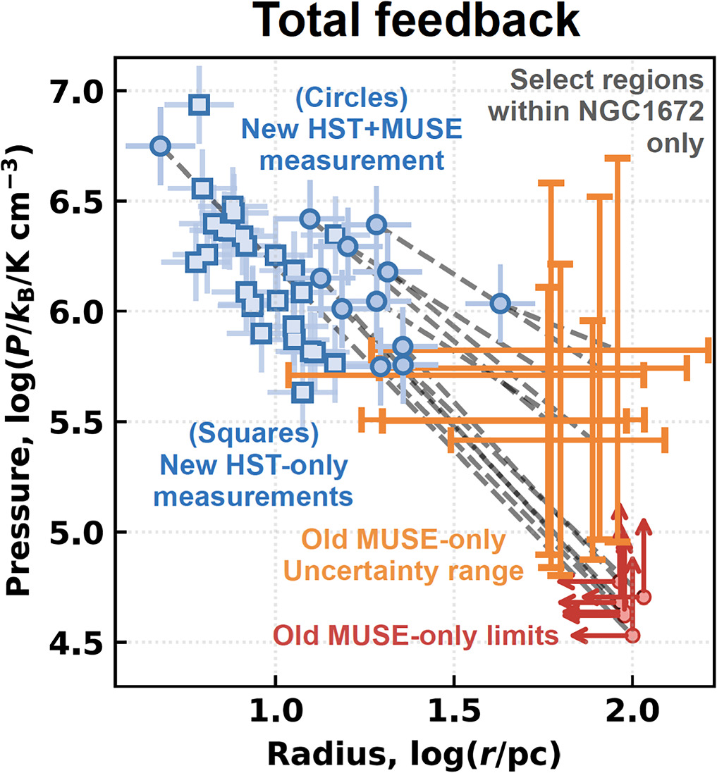
Figure 13. Demonstration of how measurements of the radii of H ii regions from HST-Hα images drastically reduce the uncertainties on stellar feedback calculations. The red points and orange bars indicate the range in size and pressure spanned by the lower and upper limits determined for H ii regions in NGC 1672 (A. T. Barnes et al. 2021). The dominant uncertainty comes from having only upper limits on H ii region size measurements in the ground-based observations. The blue points show that with the addition of HST-based size measurements, the pressure can be measured to within a factor of ∼2–3, rather than being constrained to a factor of ∼100.
Download figure:
Standard image High-resolution imagePHANGS-HST-Hα observations allow us to directly measure the radii of H ii regions, as well as the mass and age of the ionizing cluster. Direct size measurements decrease the uncertainties in the pressure estimates from a factor of ≈100 to ≈2–3, as shown by the blue data points in Figure 13. The new calculations will allow the dominant source of feedback to be identified in large samples of young clusters as a function of mass and age and across different galactic environments. The method for measuring H ii region sizes will be presented in Barnes et al. (2025, in preparation).
5.6. Leakage of Ionizing Photons from H ii Regions
Ionizing photons leak out from H ii regions and produce diffuse ionized emission (DIG) far from their birth sites. The PHANGS-HST-Hα observations are ideal for directly measuring the amount of ionizing radiation leaking out of H ii regions, fesc, right at the source. In Figures 14(e) and (f), we show examples of diffuse Hα emission escaping from H ii regions with a variety of structures, some with open shells and some without. Measurements of Hα flux outside of H ii regions (e.g., along the outer curved shell wall as shown in panel (e)) can be compared with that measured inside H ii regions to quantify fesc starting at very early ages.
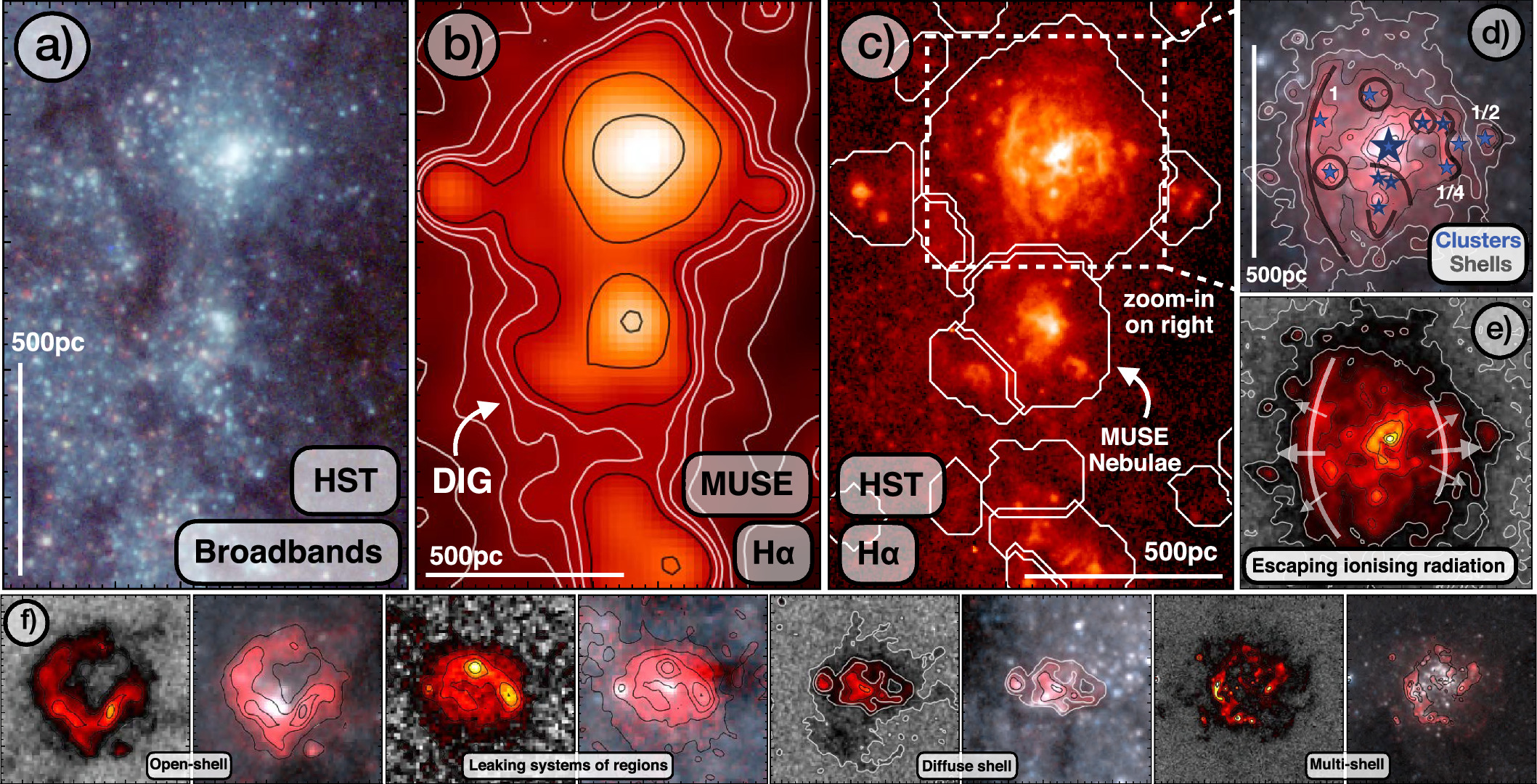
Figure 14. A star-forming complex in NGC 1672 is shown in optical broadband HST filters in panel (a) and in HST-Hα in panel (c). MUSE-defined H ii regions and DIG are outlined in panel (b). The complexity of the H ii region is highlighted in panel (d), which shows the locations of several star clusters and massive stars (star symbols) and full to partial shells of ionized gas (curved lines). Ionizing radiation leaks out of H ii regions from open shells and beyond their walls, as illustrated in panel (e). Panel (f) shows examples of different kinds of shell structures visible even in compact nebulae, many of which are leaking ionizing radiation into their surroundings. The left image in each pair shows just Hα emission, and the right image is a composite of B, V, and Hα.
Download figure:
Standard image High-resolution imageThese local measurements of fesc and H ii region morphology can be used to test predictions of how fesc depends on the molecular gas density of the local environment, which will be measured from the ALMA CO (2−1) maps. For example, simulations (Kim et al. 2019) indicate that H ii regions that form in clouds with high surface density spend a longer time (relative to the freefall time) in the embedded phase, during which the escape fraction of ionizing radiation is predicted to be small. Simulations also predict a strong (anti)correlation of the instantaneous fesc with extinction (which we will estimate from the MUSE-based Balmer decrement) and show that fesc sensitively probes gas/dust substructure driven by turbulence that creates channels for photons to emerge. The high-resolution, near-infrared images from JWST for this same sample of galaxies will also shed light on the presence of holes versus dense gas.
6. Summary
We have presented PHANGS-HST-Hα, a Cycle 30 Treasury program that forms an important part of the observational data sets gathered by the PHANGS collaboration (E. Schinnerer et al. 2019). PHANGS-HST-Hα obtained images of 19 nearby (≲20 Mpc) spiral galaxies in the F658N or F657N narrowband filter with the WFC3 camera.
Our flux calibration, continuum subtraction, and final cleaning procedures were described in detail in Section 4 and are made available online in the PyHSTHAContSub pipeline. Data products including the drizzled, aligned narrowband images and the flux-calibrated, continuum-subtracted Hα maps will be available through MAST and CADC. The error maps associated with the final continuum-subtracted Hα images will also be available. A high-level summary of the steps to create the final flux-calibrated Hα and associated error maps is given below.
- 1.Create synthetic MUSE images (Section 4.1): We created new, synthetic images from the MUSE observations to use for flux-calibrating the HST-Hα images. These were generated to mimic the narrowband F657N and F658N HST (ACS and WFC3) filters (which contain the Hα emission) and the broadband F555W and F814W (ACS and WFC3) filters (which are used to determine the continuum level).
- 2.Convert to flux density units (Section 4.2): All HST and synthetic MUSE images were converted to flux density units (erg cm−2 s−1 Å−1 pixel−1).
- 3.Smooth and regrid the HST images (Section 4.3): We smoothed and regridded the narrow- and broadband HST images to match the resolution and pixel grid of the synthetic MUSE images.
- 4.Determine background flux level from MUSE observations (Section 4.4): We performed a best linear fit between (smoothed) HST and synthetic MUSE pixel fluxes for each filter and applied the zero-point offset from these fits to the full-resolution HST images.
- 5.Continuum subtraction algorithm (Section 4.5): We calculated the contribution from the stellar continuum in our HST-Hα maps from the weighted pixel fluxes in the F555W and F814W images (where the weights (W) are calculated from the relative wavelength differences). The continuum image was subtracted from the HST-Hα image, and the units are converted to flux using the width of the Hα filter to produce the final continuum-subtracted Hα image (FHα).
- 6.Correction for [N ii] emission (Section 4.6): In addition to Hα, the F657N and F658N filters include some emission from the [N ii] λ6548 and [N ii] λ6583 emission lines. We used the MUSE spectra to determine a single correction factor for [N ii] emission for each galaxy. After this step, our pipeline produced a continuum-subtracted, Hα-only emission-line map for each galaxy.
- 7.Error maps (Section 4.7): We produced error maps associated with the reduced HST-Hα images by propagating errors in the individual pixels from the narrow- and broadband images.
- 8.Final post-processing steps (Section 4.8): These steps included corrections for remaining cosmic rays, continuum oversubtraction, and the removal of foreground stars. We also produce a final Hα mosaic image for NGC 628, since the two pointings were observed with different instruments.
In Section 5 we discussed several of the key science goals of the PHANGS-HST-Hα survey, which include improved age-dating of star clusters, size measurements of H ii regions and calculations of presupernova pressure (from warm thermal gas, radiation, and stellar winds), and direct measurements of ionizing photons leaking out of H ii regions. Catalogs of nebulae will be produced from our continuum-subtracted, flux-calibrated HST-Hα maps and released as part of an accompanying paper (A. Barnes et al. 2025, in preparation).
Acknowledgments
This research has made use of the NASA/IPAC Extragalactic Database (NED), which is operated by the Jet Propulsion Laboratory, California Institute of Technology, under contract with NASA.
The HST images produced in this paper can be found in MAST with DOI: 10.17909/t9-r08f-dq31.
M.B. gratefully acknowledges support from the ANID BASAL project FB210003 and from the FONDECYT regular grant 1211000. This work was supported by the French government through the France 2030 investment plan managed by the National Research Agency (ANR), as part of the Initiative of Excellence of Université Côte d’Azur under reference No. ANR-15-IDEX-01. O.E. acknowledges funding from the Deutsche Forschungsgemeinschaft (DFG, German Research Foundation)—project-ID 541068876. S.C.O.G. and R.S.K. acknowledge financial support from the European Research Council via the ERC Synergy grant “ECOGAL” (project ID 855130), from the German Excellence Strategy via the Heidelberg Cluster of Excellence (EXC 2181—390900948) “STRUCTURES,” and from the German Ministry for Economic Affairs and Climate Action in project “MAINN” (funding ID 50OO2206). R.S.K. is also grateful for computing resources provided by the Ministry of Science, Research and the Arts (MWK) of the State of Baden-Württemberg through bwHPC and the German Science Foundation (DFG) through grants INST 35/1134-1 FUGG and 35/1597-1 FUGG, and also for data storage at SDS@hd funded through grants INST 35/1314-1 FUGG and INST 35/1503-1 FUGG. R.S.K. also thanks the Harvard-Smithsonian Center for Astrophysics and the Radcliffe Institute for Advanced Studies for their hospitality during his sabbatical and the 2024/25 Class of Radcliffe Fellows for highly interesting and stimulating discussions. K.K. gratefully acknowledges funding from the Deutsche Forschungsgemeinschaft (DFG, German Research Foundation) in the form of an Emmy Noether Research Group (grant No. KR4598/2-1, PI Kreckel) and the European Research Council’s starting grant ERC StG-101077573 (“ISM-METALS”). G.A.B. acknowledges the support from the ANID Basal project FB210003. J.S. acknowledges support by the National Aeronautics and Space Administration (NASA) through the NASA Hubble Fellowship grant HST-HF2-51544 awarded by the Space Telescope Science Institute (STScI), operated by the Association of Universities for Research in Astronomy, Inc., under contract NAS 5-26555.
We thank the anonymous referee for a quick and helpful report.
Software: PyRAF (Science Software Branch at STScI 2012), Astrodrizzle (STSCI Development Team 2012), DOLPHOT (v2.0 A. Dolphin 2016), Photutils (L. Bradley et al. 2019), CIGALE (D. Burgarella et al. 2005; S. Noll et al. 2009; M. Boquien et al. 2019).
Appendix: Additional Checks on Background and [N ii] Correction
In Section 4 we described our pipeline steps to produce high-resolution, calibrated HST-Hα images. MUSE IFU spectroscopy was used for two purposes: to determine correct background levels for the HST-Hα images and the amount of contamination from nearby [N ii] emission lines that fall in the HST-Hα passbands. In this appendix we present additional details to justify some of the detailed choices that were made. In Figure 15 we show footprints of the HST-Hα images (red) and MUSE IFU observations (white), and we note that there is good overlap for most galaxies.
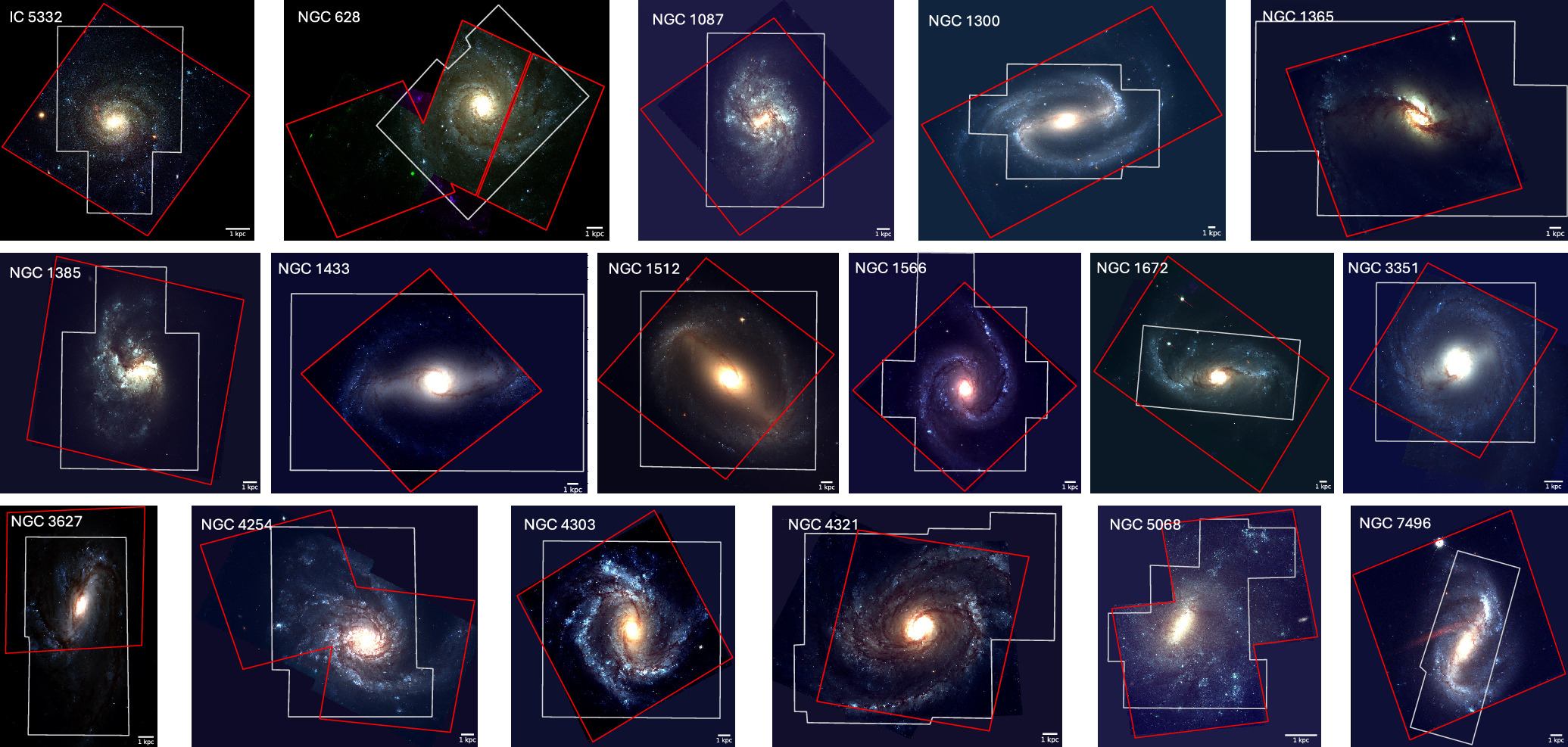
Figure 15. Footprints of the HST-Hα images (red) and MUSE IFU observations (white) are shown on HST BVI color images for the 17 galaxies that currently have Hα observations available. A 1 kpc scale bar is shown in each panel.
Download figure:
Standard image High-resolution imageA.1. Background and [N ii] Level Determination from Different Fitting Parameters
In Sections 4 and 4.4, we determined accurate background levels for the HST-Hα images and derived correction factors for the [N ii] emission-line contamination in each galaxy by calibrating them to the MUSE spectroscopic observations. In both cases, we allowed the slope and intercept to be free parameters in the fits; however, we only applied the offset in the former case (background correction) and the slope in the latter ([N ii] correction). In this section, we explore the impact on the derived correction factors of fixing the slope to unity or the offset to zero, following the same procedures outlined in Sections 4 and 4.4.
Columns (2), (3), and (4) of Table 6 report the background level fits (the y-intercept) obtained when the slope is fixed to unity rather than treated as a free parameter. Column (5) of Table 6 lists the correction factors for the [N ii] emission lines when the y-intercept is fixed to zero. We find that these values, derived under fixed-slope or fixed-intercept conditions, are broadly consistent with those obtained when both slope and offset are allowed to vary freely.
Table 6. Fitting Results for the Background Correction in Each of the HST Filters (Section 4.4), and the Correction Factor for the [N ii] λ6548 and [N ii] λ6583 Line Contamination in the Hα Images (Section 4.6)
| Galaxy | Background Corrections | [N ii] Correction | ||
|---|---|---|---|---|
| (erg s−1 cm−2 Å−1 arcsec−2) | ||||
| F555W | F65XN | F814W | Factor | |
| IC 5332 | −337.96 | 1838.07 | −227.22 | 1.10 |
| NGC 628-C | −483.21 | −516.31 | −340.13 | 1.35 |
| NGC 628-E | −149.63 | 1579.62 | −175.47 | 1.19 |
| NGC 1087 | −272.16 | 828.05 | −181.57 | 1.19 |
| NGC 1300 | −51.87 | −94.14 | −60.14 | 1.33 |
| NGC 1365 | −882.44 | 438.51 | −723.04 | 1.27 |
| NGC 1385 | −249.12 | 832.78 | −190.41 | 1.23 |
| NGC 1433 | −620.67 | −663.53 | −544.69 | 1.43 |
| NGC 1512 | −198.70 | 1435.68 | −128.10 | 1.03 |
| NGC 1566 | −1022.72 | 1544.01 | −577.03 | 1.03 |
| NGC 1672 | −250.62 | −363.09 | −171.77 | 1.39 |
| NGC 2835-S | −505.99 | 715.02 | −369.64 | 1.00 |
| NGC 3351 | −294.10 | 329.90 | −229.84 | 1.08 |
| NGC 3627 | −1098.37 | −236.31 | −838.19 | 1.15 |
| NGC 4254 | −77.69 | 93.99 | −229.99 | 0.97 |
| NGC 4303 | −1140.68 | −566.77 | −900.57 | 0.97 |
| NGC 4321 | −801.34 | 566.60 | −713.40 | 1.28 |
| NGC 4535 | −648.72 | 605.50 | −531.96 | 1.17 |
| NGC 5068 | −331.19 | −143.40 | −202.55 | 1.10 |
| NGC 7496 | −172.27 | 549.13 | −134.12 | 1.25 |
Note. Here we have fixed the slope of the fit for the background correction to unity and the intercept for the [N ii] correction to zero (see Table 4, where these are left as free parameters in our fitting).
Download table as: ASCIITypeset image
A.2. HST-to-MUSE Hα Fluxes as a Function of Nebular Properties
In Figure 12, for NGC 628 c we showed the ratio of HST to MUSE Hα fluxes versus the MUSE Hα flux, MUSE Hα velocity, galactocentric radius, and the Hα equivalent width measured directly from the MUSE spectra. There is some range in the results for the galaxies in our sample, so in Figure 16 we present the exact same measurements for NGC 1566 (top panels) and NGC 4303 (bottom panels). These plots allow a deeper understanding of any systematic variations in the HST-to-MUSE flux ratios, as well as the reliability of cross-calibration for Hα measurements across different galactic conditions.
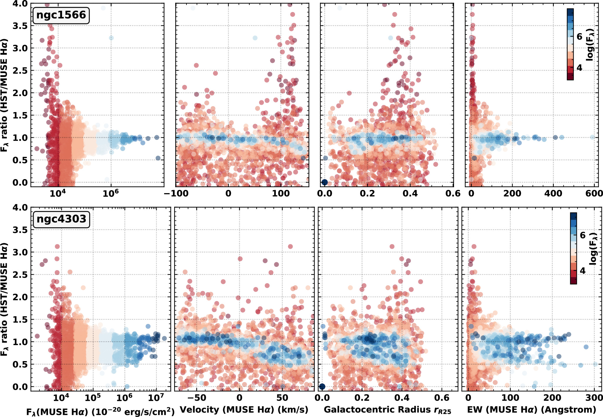
Figure 16. The ratio of the HST to MUSE Hα fluxes checked against other nebula properties for NGC 1566 and NGC 4303. We show (from left to right) the Hα flux ratio vs. the MUSE Hα flux, MUSE Hα velocity, galactocentric radius, and the Hα equivalent width measured directly from the MUSE spectra. There is no obvious trend in the flux ratio with Hα velocity or galactocentric distance (middle two panels), although for NGC 4303 there appears to be a decline in the HST-to-MUSE flux ratio at higher velocities (>100 km s−1), likely due to the filter response.
Download figure:
Standard image High-resolution imageUnlike the results shown in the main text for NGC 628 (Figure 11), here we observe a trend of decreasing HST-to-MUSE flux ratios at higher velocities (>50 km s−1), which is particularly pronounced for NGC 4303 (see also >100 km s−1 for NGC 1566). This effect is likely due to the position of NGC 4303 at the edge of the F658N filter response curve (see Figure 3), which could lead to a reduction in the effective Hα transmission at higher velocities relative to MUSE. In contrast, NGC 628 does not show this trend in Figure 11, supporting the hypothesis that proximity to the filter band edge influences flux measurements in cases with high nebular velocities. To correct for this, velocity-dependent flux correction will be included in a future version of the pipeline.
A.3. F555W Filter versus F550M and F547M for Continuum Subtraction
The F555W filter was used (along with F814W) to estimate and subtract the continuum level in the narrowband images. This filter may suffer contamination from strong emission lines such as [O iii] and potentially introduce residuals in continuum subtraction that affect the derived flux maps when compared with the narrower F550M or F547M filters. We tested the impact of using the F550M or F547M filters rather than the F555W filter by using data available for NGC 1672 and NGC 3351. We ran the full pipeline, which includes the background subtraction and [N ii] correction steps (using the F550M or F547M filter transmission curves applied to the MUSE cubes), as well as using the filters for the continuum subtraction.
Figure 17 shows the resulting maps and a comparison of the per-pixel fluxes. We observe that in NGC 1672 the F555W filter appears to have some minor residual continuum in the image when compared to the F550M filter subtraction, which appears predominantly toward the center of the galaxy. This is consistent with expectations that [O iii] emission might contaminate the F555W filter more significantly in regions with strong ionizing sources. Nonetheless, overall we see a very close one-to-one match of the fluxes across the galaxy (see the top right panel of Figure 17). In NGC 3351 we see that there is a slight shift to lower values for the F547M filter subtraction when compared to the F555W subtraction (see dotted line in Figure 17), though this appears to be an effect of poor background subtraction in the F547M filter rather than due to line contamination, which would predominantly affect smaller scales. Overall, we found that switching to the F547M or F550M filters makes little difference to the final flux-calibrated, continuum-subtracted images, indicating that line contamination does not significantly propagate into the final products for these galaxies.
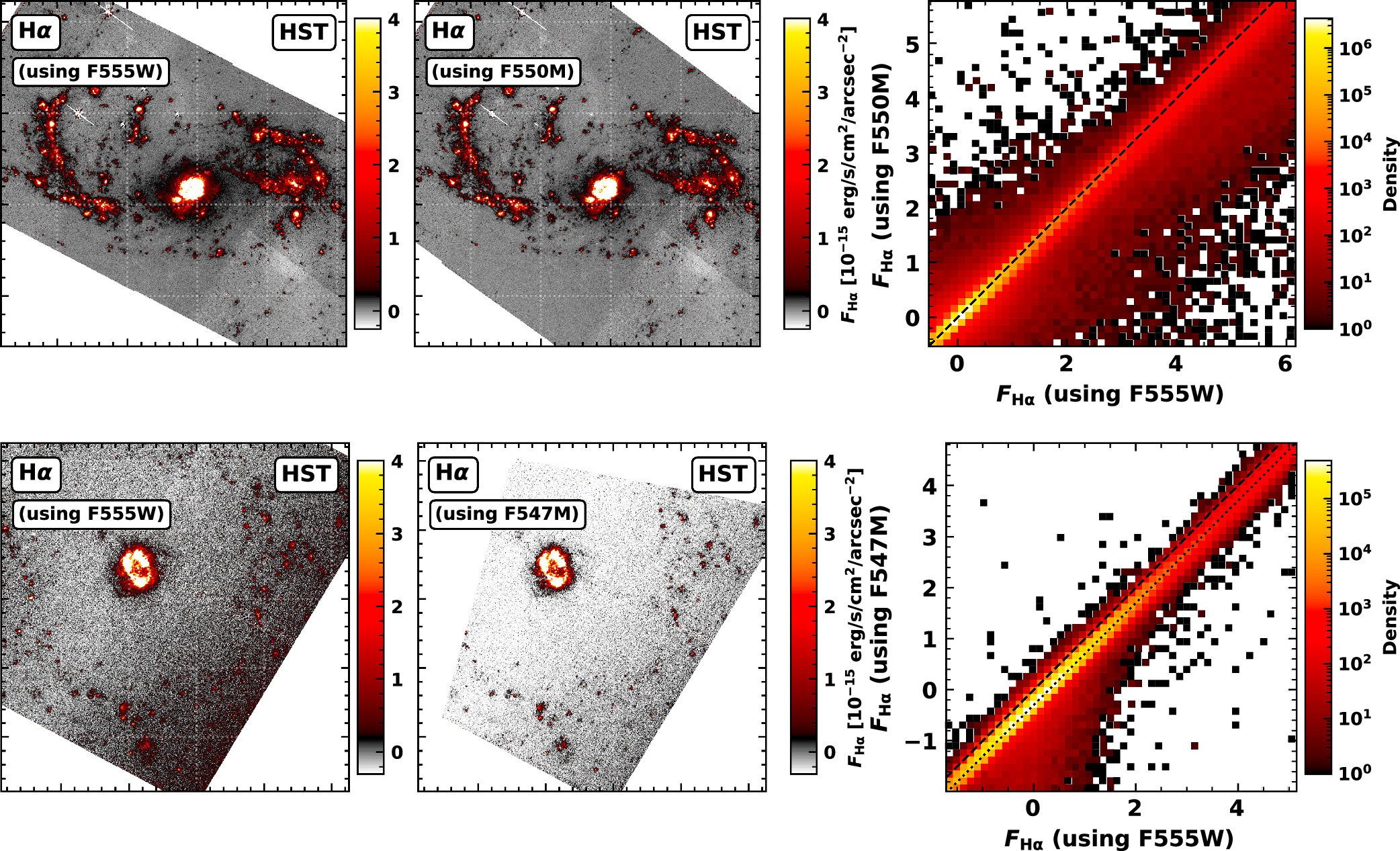
Figure 17. Difference between using the F555W vs. F550M and F547M filters for continuum subtraction. The top row shows the difference between using the F555W (left) and F550M (middle) filters for continuum subtraction in NGC 1672, while the bottom row shows the difference between F555W and F547M for NGC 3351. The right panels show 2D histogram density plots of the Hα flux at each pixel for both cases. Overlaid is a dashed line showing the y = x relation, and the dotted line in the bottom panel shows an offset of y = x − 0.3.
Download figure:
Standard image High-resolution imageFootnotes
- 30
- 31
See version 1 release of the code used throughout this work in the following link 10.5281/zenodo.14610187.
- 32
- 33
- 34
- 35
- 36
Note that the HST-filtered MUSE images have already been corrected for foreground Galactic extinction.
- 37
Note that these images were used, and not, e.g., the ratio of the MUSE image Hα/([N ii] λ6548 + [N ii] λ6583), as these synthetic MUSE images retain the variation in the filter transmission, due to the velocity field of the galaxies.
- 38
As we do not correct for the offset of the fit in this case (as opposed to the background subtraction, where we used a similar correction but only applied the offset; see Section 4.4), we also investigate the effect of fixing the offset to zero in this [N ii] correction fitting procedure. However, doing so results in only a minor change in the correction (see Table 6 in the Appendix).
- 39
In practice, we iterate three times the interpolating function with a kernel with a standard deviation of 1 pixel.
- 40
- 41