Abstract
We present the discovery of Kepler-88 d (
 ,
,  ,
,  ) based on six years of radial velocity (RV) follow-up from the W. M. Keck Observatory High Resolution Echelle Spectrometer spectrograph. Kepler-88 has two previously identified planets. Kepler-88 b (KOI-142.01) transits in the NASA Kepler photometry and has very large transit timing variations (TTVs). Nesvorný et al. performed a dynamical analysis of the TTVs to uniquely identify the orbital period and mass of the perturbing planet (Kepler-88 c), which was later was confirmed with RVs from the Observatoire de Haute-Provence (OHP). To fully explore the architecture of this system, we performed photodynamical modeling on the Kepler photometry combined with the RVs from Keck and OHP and stellar parameters from spectroscopy and Gaia. Planet d is not detectable in the photometry, and long-baseline RVs are needed to ascertain its presence. A photodynamical model simultaneously optimized to fit the RVs and Kepler photometry yields the most precise planet masses and orbital properties yet for b and c:
  ,
,  ,
,  , and
, and  . The photodynamical solution also finds that planets b and c have low eccentricites and low mutual inclination, are apsidally anti-aligned, and have conjunctions on the same hemisphere of the star. Continued RV follow-up of systems with small planets will improve our understanding of the link between inner planetary system architectures and giant planets.
1. Introduction
The NASA Kepler mission detected hundreds of systems with multiple transiting planets (Lissauer et al. 2011; Fabrycky et al. 2014; Rowe et al. 2014), providing insight into one of the most common modes of planet formation. One unexpected attribute of the Kepler planetary systems is that planets in or very near mean-motion resonances are rare (Fabrycky et al. 2014). The prevalence of planets that are not in mean-motion resonances seems at odds with examples from our solar system (e.g., the Galilean moons) and resonant chains of giant exoplanets detected in radial velocity (RV) surveys (e.g., Marcy et al. 2001). Resonant architectures are expected to arise when planet pairs migrating convergently become trapped in the energetically favorable configuration of mean-motion resonance. Since viscous migration in a disk is often invoked to explain the prevalence of volatile-containing planets within 1 au, the dearth of resonant planetary architectures in the compact Kepler planetary systems is an unsolved puzzle.
Kepler-88 (KOI-142) is a rare example of a planetary system very near a mean-motion resonance. The system has only one transiting planet, Kepler-88 b (KOI-142.01), a sub-Neptune-sized planet with an orbital period of 10.95 days. Kepler-88 b is perturbed by a non-transiting giant planet with a period of 22.26 days, Kepler-88 c (KOI-142.02, Nesvorný et al. 2013). The resonant conjunctions of the sub-Neptune and giant planet produce large transit timing variations (TTVs), which have an amplitude of half a day (5% of the orbital period of the transiting planet, see Figure 1). These very large TTVs led to the nickname “the king of TTVs” for the Kepler-88 system (Steffen et al. 2012a) and have been identified in various TTV catalogs (e.g., Ford et al. 2011; Steffen et al. 2012a; Mazeh et al. 2013; Holczer et al. 2016).
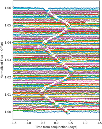
Figure 1. Kepler long-cadence photometry of Kepler-88 near expected times of conjunction for Kepler-88 b (P = 10.95 days), with individual transits offset vertically (epoch increases from bottom to top, and the colors disambiguate adjacent epochs). The TTVs of amplitude 0.5 day are readily identifiable.
Download figure:
Standard image High-resolution imageThe Kepler-88 b TTVs were first explained dynamically in Nesvorný et al. (2013, hereafter N13). In an N-body dynamical fit, they found that (1) the perturber of the Neptune-sized planet is at  days, (2), the mass of the perturber is
  , (3) the eccentricities of the 11 and 22 day planets are small but non-zero (
 ,
,  ), and (4) the orbits of the resonant planets are apsidally anti-aligned (
 ). N13 also found non-negligible transit duration variations (TDVs) of the transiting planet, which provided a constraint on the mutual inclination of the two planets.
Shortly thereafter, Barros et al. (2014) used the Observatoire de Haute-Provence (OHP) telescope and SOPHIE high-resolution echelle spectrograph to measure RVs of the Kepler-88 system. With one season of RVs, they confirmed the presence of a 
 planet with an orbital period of 22.10 ± 0.25 days. This was the first time that RVs confirmed an accurate and precise prediction of the location and mass of a non-transiting exoplanet from TTVs.
In this paper, we present RVs of Kepler-88 from the W. M. Keck Observatory High Resolution Echelle Spectrometer (HIRES) taken between the years 2013 and 2020. Our RVs confirm the existence, mass, and orbital period of the giant planet at 22.26 days. We also detect another giant planet in the system, Kepler-88 d, at an orbital period of  , with minimum mass (
 ) of
) of  and an eccentricity of
  . The high mass and eccentricity of Kepler-88 d indicate that it has likely been an important dynamical component in this planetary system’s history. To identify accurate dynamical parameters for all of the known bodies in the system, we simultaneously fit the Kepler photometry, Keck-HIRES RVs, and OHP-SOPHIE RVs of Kepler-88 with multiple N-body codes.
This paper is organized as follows. In Section 2, we present our observing strategy and the Keck-HIRES RVs, literature RVs, and stellar properties. In the following sections, we explore the RV data with increasingly complex models and supplementary data. In Section 3, we present a three-planet Keplerian model to the RVs. In Section 4, we present the results of a simultaneous N-body fit to the RVs and TTVs. In Section 5, we perform simultaneously an N-body fit to the RVs and Kepler photometry (a photodynamical fit). In Section 6, we present the main results from our analyses. In Section 7, we discuss how our results affect our interpretation of the history of this planetary system, and how this system adds to the small but growing list of systems with characterizations from both RV and TTV analyses. In Section 8 we conclude.
2. Keck-HIRES Spectra
2.1. Radial Velocities
We obtained  RVs of Kepler-88 on the HIRES spectrograph (Vogt et al. 1994) at the W. M. Keck Observatory between the years 2013 and 2020. We used the standard HIRES setup of the California Planet Search (see Howard et al. 2010 for details). Spectra were obtained using HIRES in the red-collimation mode with a warm molecular iodine gas cell in the light path for wavelength calibration. We used the C2 decker (
 , R = 60,000) to enable sky-subtraction for this relatively faint (V = 13.8) target. Since the target was faint, we only observed in good conditions (seeing <1
5, clear to thin clouds). For each spectrum, we achieved a signal-to-noise ratio of at least
 to ensure that our Doppler pipeline would deliver RVs with errors of
  (Howard & Fulton 2016).
We observed an iodine-free template spectrum bracketed by observations of rapidly rotating B-type stars to enable a deconvolution of the stellar spectrum from the spectrograph point-spread function (PSF). We then forward modeled our RV spectra with the deconvoled template stellar spectrum plus a night-specific model of our PSF convolved with an atlas iodine spectrum. We also used the blue HIRES chip to extract a Mt. Wilson  value for each HIRES observation. Our Keck-HIRES RVs and
  values, plus the SOPHIE RVs from the literature, are presented in Table 1.
Table 1. Kepler-88 RVs
| Time | RV |

|
SHK | Inst |
|---|---|---|---|---|
| (BJD — 2454900) | (m s−1) | (m s−1) | ||
| 1575.047908 | −35.7 | 2.8 | 0.142 | HIRES |
| 1575.40947 | 42.0 | 10.0 | SOPHIE | |
| 1575.992695 | −36.7 | 2.4 | 0.155 | HIRES |
| 1577.892731 | −52.9 | 2.5 | 0.147 | HIRES |
| 1579.027079 | −81.7 | 2.6 | 0.122 | HIRES |
| ⋯ | ⋯ | ⋯ | ⋯ | ⋯ |
Note. Times are in BJD — 2454900.0. SOPHIE RVs are from Barros et al. (2014); HIRES RVs are from this work. The SOPHIE RVs have had 20465.0  added, with respect to the values published in Barros et al. (2014), for easier zero-point calibration. The RV uncertainties do not include RV jitter.
Only a portion of this table is shown here to demonstrate its form and content. A machine-readable version of the full table is available.
Download table as: DataTypeset image
2.2. Stellar Parameters
The stellar properties of Kepler-88 were determined based on our high signal-to-noise template spectrum in combination with the Gaia parallax and Two Micron All Sky Survey (2MASS) photometry (Fulton & Petigura 2018). The stellar temperature is 5466 ± 60 K and with [Fe/H] =  , the star is slightly metal-rich. The star has a similar mass but slightly smaller radius than the Sun (
 =
=  ,
,  =
=  ).
).
Because the transit of planet b combined with dynamical information about the planet constrains the density of the star, we used a photodynmical fit to update the stellar characterization (e.g., Vanderburg et al. 2017, see Section 5.2). We used the best-fit values and uncertainties for the stellar mass and radius from Fulton & Petigura (2018) as priors in our photodynamical fit. After our photodynamical fit, the best-fit stellar mass and radius are  =
=  and
and  =
=  . The precision of the stellar radius determination was improved through the photodynamical fit, suggesting that the transits provide information about the stellar density and hence the stellar radius.11
Of the stellar parameters reported here, only the stellar mass is dependent on isochrone fitting (see Fulton & Petigura 2018 for details). We caution that the formal error in the mass reported here does not account for systematic differences between the stellar isochrones formulated by different research groups, and so the reported error in the stellar mass (and hence density) might be underestimated.
3. Keplerian Fit
The RVs of Kepler-88 show long-term variation from a planetary companion at ∼4 yr (see Figures 2–4). The discovery of this companion is the result of the long baseline (currently six years) of Keck-HIRES RVs. The 4 yr RV variation does not correlate with  variability, strongly disfavoring a stellar activity cycle as the source of the RV signal.
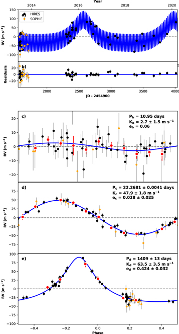
Figure 2. (a) RVs of Kepler-88 from Keck-HIRES (black) and OHP-SOPHIE (orange), and their errors (including jitter) as a function of time. The best-fit three-planet Keplerian solution is shown in blue. (b) The residuals. (c) The RVs phase-folded to the linear ephemeris of planet b, with the other Keplerian signals removed. Binned average RVs and their uncertainties are shown in red. The RVs alone do not detect the mass of planet b, but planet b clearly exists from its transits. (d) Same as above, but for planet c, which does not transit. (e) Same as above, but for planet d, which does not transit. With a period of 1400 days, planet d is not detected in the TTVs, and so only the RVs provide a useful determination of its orbital properties.
Download figure:
Standard image High-resolution image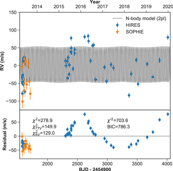
Figure 3. Top: Kepler-88 RVs from Keck-HIRES (blue) and OHP-SOPHIE (orange). The best two-planet N-body fit to the RVS and TTVs (Kepler-88 b and c) is shown in black. Bottom: the RV residuals. There is a strong residual RV signal near 1400 days. The χ2 values of the fit to the TTVs and RVs are given, as are the penalty adjusted  and BIC.
Download figure:
Standard image High-resolution image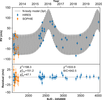
Figure 4. Same as Figure 3, but showing the best three-planet N-body model and residuals (note the different y-axis ranges). The inclusion of the third planet substantially reduces the RV residuals and improves (reduces) the BIC.
Download figure:
Standard image High-resolution imageTo obtain initial estimates of the orbital properties of all three planets, we fit the RVs from both HIRES and SOPHIE with a three-planet Keplerian model using RadVel (Fulton et al. 2018). Since the innermost planet is very low mass, we fixed its orbital period and transit time at the best linear-ephemeris values as determined from the Holczer et al. (2016) TTVs (Pb = 10.95 days), and kept its eccentricity fixed. We allowed the five orbital elements, P, Tp,  ,
,  , and
, and  , to vary for planets c and d, as well the HIRES RV zero-point (γHIRES), the SOPHIE RV zero-point (γSOPHIE), and the RV jitter for each telescope (σHIRES), (σSOPHIE). Our priors were 0 < e < 1 and K > 0 for all planets. We explored these parameters with a Markov Chain Monte Carlo (MCMC) analysis, the results of which are in Tables 2 and 3.
Table 2. RV-only Keplerian MCMC Posteriors
| Parameter | Credible Interval | Maximum Likelihood | Units |
|---|---|---|---|
| Orbital Parameters | |||
| Pb | ≡10.9531 | ≡10.9531 | days |
| Tconjb | ≡175.1591 | ≡175.1591 | JD |
| eb | ≡0.06 | ≡0.06 | |
| ωb | ≡−3.1306 | ≡−3.1306 | radians |
| Kb |

|
2.8 | m s−1 |
| Pc |

|
22.2679 | days |

|

|
172.27 | JD |
| ec |

|
0.02 | |

|

|
−0.5 | radians |
| Kc |

|
47.9 | m s−1 |
| Pd |

|
1409 | days |

|
1325 ± 21 | 1327 | JD |
| ed |

|
0.422 | |
| ωd |

|
0.033 | radians |
| Kd |

|
63.7 | m s−1 |
| Other Parameters | |||

|

|
42.6 | m s−1 |

|
−4.0 ± 1.3 | −4.0 | ms−1 |

|
≡0.0 | ≡0.0 | m s−1 d−1 |

|
≡0.0 | ≡0.0 | m s−1 d−2 |
| σSOPHIE |

|
6.4 |

|

|

|
5.41 |

|
Note. BJD0 = 2454900.
Download table as: ASCIITypeset image
Table 3. RV-only Keplerian Derived Posteriors
| Parameter | Credible Interval | Maximum Likelihood | Units |
|---|---|---|---|
| ab |

|
0.09687 | au |

|

|
3.4 |

|
| ρb |

|
0.4 | g cm−3 |
| ac | 0.154 ± 0.001 | 0.156 | au |

|

|
0.671 | MJup |
| ad | 2.45 ± 0.02 | 2.458 | au |

|
3.15 ± 0.15 | 3.14 | MJup |
Download table as: ASCIITypeset image
The RVs place tight constraints on planet masses  c (
c (
 ) and
) and  d (
d ( ), but provide very little information about Mb. This is because the transiting planet is small and the star is faint; many RVs are needed in this regime to obtain accurate and precise planet masses. As we show below, however, incorporating the TTVs or a full photodynamical model dramatically improves our constraint on the masses and orbits of Kepler-88 b and c with respect to the RV-only solution.
4. N-body Fit to TTVs + RVs
There is an important distinction between an N-body fit (e.g., in Figures 3 and 4) versus a multiple-Keplerian fit (e.g., Figure 2): N-body fits include planet–planet interactions, whereas Keplerian fits do not. A detailed N-body analysis is necessary to accurately model the positions and velocities of the Kepler-88 bodies because the two inner planets are near resonance.
We used the N-body code TTVFast (Deck et al. 2014) to simultaneously reproduce the TTVs and RVs in the Kepler-88 system. For this analysis, we used the TTVs published in Holczer et al. (2016), which are measured from the Kepler long-cadence photometry. Our optimization algorithms included least-squares minimization and MCMC analysis. We considered a two-planet model (planets b and c only) and a three-planet model (planets b, c, and d), fitting the TTVs alone, and then the RVs and TTVs simultaneously. We varied the masses, orbital periods, eccentricities and arguments of pericenter (via parameters  and
and  ), and mean anomalies for each of the planets at epoch BJD = 2454954.62702, as well as the inclination and longitude of ascending node for planet c, and an RV zero-point jitter for each spectrograph. We penalized high values of RV jitter in our minimization function
  :
:

where  is the quadrature sum of the ith individual RV error and the RV jitter of the corresponding spectrograph, and χ2 is the usual statistic

We compared the goodness of fit of our four models using the Bayesian information criterion (BIC):

where N is the number of data points (TTV alone or RV + TTV, depending on which data were used) and Nvarys is the number of variables. Note that we use  instead of χ2 in calculating the BIC so that the penalty for large RV jitters is included in our model comparison. The χ2 values, degrees of freedom, and BICs from our four-way analysis are summarized in Table 4. If only the TTVs are fit, a two-planet model is adequate for fitting the data, based on the similar values of the BIC for the two- and three-planet models (ΔBIC = 24, in favor of the two-planet model). However, in fitting the TTVs combined with the RVs, a three-planet model is strongly preferred, with ΔBIC = −144. To illustrate the better performance of the three-planet model, the RVs are shown with our best two-planet fit (Figure 3) and our best three-planet fit (Figure 4). The TTVs and our best three-planet fit are shown in Figure 5 (upper panel). The best-fit planet masses and orbits from the TTV and TTV+RV analyses are within 1σ of the values we find in our photodynamical analysis, which is presented in Section 5.
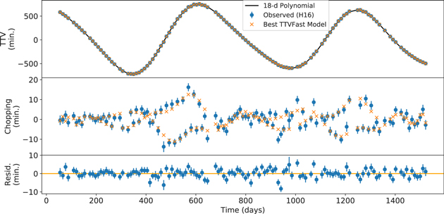
Figure 5. Top: the observed TTV signal from Holczer et al. (2016; blue dots), our best-fit model produced with TTVFast (orange crosses), and an 18° polynomial fit to the observed TTVs (black line). Middle: the high-frequency chopping signal was separated from the low-frequency TTV signal by subtracting the polynomial fit, for both the observed transit times (blue dots) and modeled TTVs (orange crosses). Both the observed and modeled chopping signals have amplitudes that vary with the phase of the TTV super-period. Bottom: the residuals (observed minus modeled transit time).
Download figure:
Standard image High-resolution imageTable 4. Model Comparison
| Model | Data | Nvarys |

|

|
σHIRES | σSOPHIE |

|
DOF | BIC |
|---|---|---|---|---|---|---|---|---|---|
( ) ) |
( ) ) |
||||||||
| Two planets | TTVs | 16 | 149.5 | 0 | ⋯ | ⋯ | 150 | 105 | 226 |
| Three planets | TTVs | 21 | 149.6 | 0 | ⋯ | ⋯ | 150 | 100 | 250 |
| Two planets | TTVs + RVs | 16 | 150 | 129 | 20.0 | 9.6 | 703 | 160 | 786 |
| Three planets | TTVs + RVs | 21 | 150 | 50 | 6.6 | 8.1 | 534 | 155 | 642 |
| Three planets, control | Phot + RVs | 26 | ⋯ | 73.0 | 6.5 | 6.2 | 1564297 | 1564457 | 1564668 |
| Three planets, ic flipped | Phot + RVs | 26 | ⋯ | 45.5 | 6.5 | 6.2 | 1564330 | 1564457 | 1564701 |
| Three planets, id = 30° | Phot + RVs | 26 | ⋯ | 75.6 | 6.5 | 6.2 | 1564303 | 1564457 | 1564674 |
Note. There are 121 TTV data, 55 RV data, and 1564429 photometric data.  and σSOPHIE are the HIRES and SOPHIE jitter terms, respectively, which are added to the intrinsic RV errors in quadrature.
Download table as: ASCIITypeset image
4.1. Chopping Signal
In systems that are not very close to resonance and/or have large TTV uncertainties compared to the timing precision, only the low-frequency TTV super-period is detected. This low-frequency signal contains information about the mass ratio of the planets, but the absolute masses are degenerate with the eccentricities of the planets (Lithwick et al. 2012). However, in systems with high signal-to-noise TTV measurements like Kepler-88, it is possible to detect a higher-frequency signal: the synodic chopping signal. This signal abruptly changes direction after conjunctions between the transiting and perturbing planet (Agol & Fabrycky 2018). The chopping signal is therefore expected to occur at the synodic period, or

In Kepler-88, the expected chopping period is Pchop = 21.5 days.12 We identified the chopping signal by fitting the Holczer et al. (2016) TTVs with a high-order polynomial13 (degree 18) and subtracted this polynomial fit from the TTVs (Figure 5, middle panel, blue points). The high-frequency variations in the TTVs show a characteristic chopping signal. Note that the strength of the chopping comes and goes at different phases of the TTV super-period. This episodic strength of the chopping signal is well reproduced by our best-fit model (orange crosses).
We used a Lomb–Scargle periodogram to identify the super-period of the TTVs at 611 days (Figure 6, top). After we removed the high-degree polynomial, the Lomb–Scargle periodogram of the TTV residuals had its highest peak at P = 20.9 or 23 days (which is the mirror reflection of 20.9 days about the Nyquist frequency), and a peak at the expected chopping signal at 21.5 days (bottom). Note that peak periods are reflected about the Nyquist frequency,  day−1.
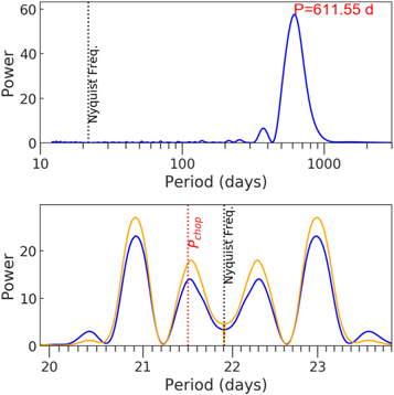
Figure 6. Top: the Lomb–Scargle periodogram of the TTV signal has a peak at 611 days, the super-period of the Kepler-88 TTVs. Bottom: the Lomb–Scargle periodogram of the chopping signal (after removing the TTV super-period) of both the observed TTVs (blue) and our best-fit model (orange). The predicted chopping signal is at 21.5 days (below the Nyquist frequency), but the strongest frequency is at 20.9 (or 23) days. The peak at 20.9 days corresponds to the 2:3 mean-motion resonance of planets b and c.
Download figure:
Standard image High-resolution imageTo better understand the origin of the peak at 20.9 or 23 days, we examined the behavior of the TTV chopping signal on longer timescales. We simulated TTVs for 50 yr using the best-fit parameters and the N-body integrator rebound (Rein & Tamayo 2016; Figure 7, top panel). The long-term TTVs have both the a super-period at 611 days, and a super–super period at 20.5 yr (7500 days). We used a fast Fourier transform to construct a low-pass filter and subtracted the filter from the model, thus obtaining the chopping signal (bottom panel). In Figure 8, we show the Lomb–Scargle periodogram of the chopping signal based on different numbers of consecutive transits. A periodogram of the 221 transits from the middle of the simulated chopping signal yields peaks at the chopping frequency (21.56 days) and 20.9/23 days. Including more transits increases the power at these distinct periods, and reveals splitting of the 20.9/23 days period. The peak at 20.91 days is at  , i.e., the 2:3 resonance.14
The splitting appears consistent with the super–super period, as the peaks occur at 20.91 and
, i.e., the 2:3 resonance.14
The splitting appears consistent with the super–super period, as the peaks occur at 20.91 and  days.
days.
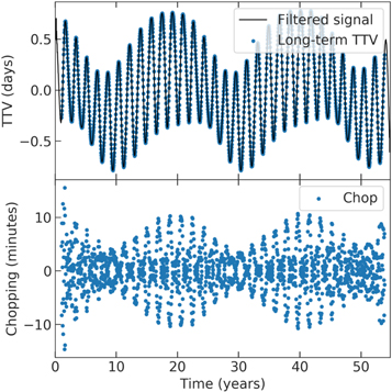
Figure 7. Top: long-term TTVs of Kepler-88 b predicted from our best-fit model (blue points) and a fast Fourier transform of the TTVs (black line). In addition to the 600 days super-period, there is a 20 yr super–super period. Bottom panel: the long-term chopping signal is computed by subtracting the fast Fourier transform from the TTVs in the upper panel. The chopping signal amplitude varies on the timescales of the TTV super-period and super–super period.
Download figure:
Standard image High-resolution image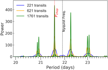
Figure 8. Lomb–Scargle periodogram of the long-term chopping signal from Figure 7 based on the middle 221 (blue), 621 (orange), or 1761 (green) consecutive transits. With only 221 transits, the peaks at 21.5 days (the synodic chopping signal), its reflection about the Nyquist frequency, and the peaks 20.9/23 days are visible. With additional transits, the power at each of these peaks grows. The peaks at 20.9/23 days split, but the peaks at the synodic chopping period and its Nyquist reflection do not.
Download figure:
Standard image High-resolution imageTo investigate the origin of the super–super period, we plotted the evolution of  and
and  in a simulation with just the inner two planets (Figure 9), and confirmed that the super–super period (20.5 yr) is the timescale of precession of planet b due to planet c.15
There are approximately 11 retrograde epicycles during the 20.5 yr precession; each of these epicycles corresponds to a TTV super-period of ∼611 days.
in a simulation with just the inner two planets (Figure 9), and confirmed that the super–super period (20.5 yr) is the timescale of precession of planet b due to planet c.15
There are approximately 11 retrograde epicycles during the 20.5 yr precession; each of these epicycles corresponds to a TTV super-period of ∼611 days.
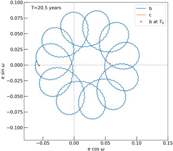
Figure 9. Parametric evolution of  ,
,  , in a simulation with just the inner two planets. In 20.5 yr, planet b traces a flower/spirograph pattern through
  ,
,  space. Each epicyclic petal is traced in 611 days (the super-period of the TTVs), and the full flower is completed in 20.5 yr (the super–super period of the TTVs). Note that the precession of the super period and the super–super period have opposite signs. The small zigzags are at the timescale of synodic chopping.
Download figure:
Standard image High-resolution image5. Photodynamical Fit to Transits and RVs
A photodynamical fit is produced by optimizing an N-body model to fit photometry (and in this case also RVs). Unlike a simultaneous fit to TTVs + RVs, the photodynamical fit must reproduce the transit time and also the transit depth, duration, and shape at each epoch. It is computationally more expensive than a fit to TTVs, but also potentially more informative, as it enables an exploration of the inclinations (i) and longitudes of ascending node (Ω) of the planets, which can be constrained by the transit depths and durations.
To improve upon the RV + TTV solution, we used an iterative photodynamical forward-model to simultaneously fit the photometry and RVs of the Kepler-88 system. We used the code Phodymm, which has previously been used to model and fit photometry from the Kepler prime mission in Kepler-223, (Mills et al. 2016), Kepler-444 (Mills & Fabrycky 2017a), and Kepler-108 (Mills & Fabrycky 2017b), and the combined Kepler prime photometry and Keck-HIRES RVs in Kepler-25, Kepler-65, and Kepler-68 (Mills et al. 2019). Phodymm is a Runge–Kutta N-body integrator that can simultaneously forward-model photometry and RVs for N planets and one star. The transit shape is reproduced with the prescription given in Pál et al. (2011). This model includes a transit shape described by Mandel & Agol (2002), with the quadratic limb-darkening coefficients of Claret (2000). For simplicity, Phodymm assumes that the velocity of the planet is constant during transit. For input parameters, it can accept Cartesian, asterocentric, or Jacobi coordinates. We used the Jacobi orbital elements: orbital period P, time of conjunction Tc, eccentricity e, inclination i, longitude of ascending node Ω, and argument of periastron passage ω, all of which were defined at epoch BJD = 2454954.62702. Additional input parameters were the planet-to-star radius ratio  /
/ , and planet mass
  for each planet, as well as the stellar mass
  , radius
  , dilution D, and quadratic limb-darkening coefficients c1 and c2.
5.1. Photometry
We downloaded the photometry of Kepler-88 (KOI-142, KIC 5446285) obtained during the Kepler prime mission from the MAST archive.16 Where available (quarters 4–17), we used short-cadence data; we used long-cadence data elsewhere. We detrended the photometry in the manner of Mills & Fabrycky (2017b). First, we segmented the lightcurve into chunks of approximately one day, masking any transits within each chunk. We then fit the photometry in each chunk with a cubic polynomial to model the continuum, including both systematic effects and stellar rotation. We divided the observed flux by our continuum model to obtain normalized photometry. We multiplied all the uncertainties by a scale factor such that the out-of-transit reduced χ2 is 1.0, for both long cadence and short cadence independently.
5.2. Photodynamical Fit
Since no stellar companions are known, we fixed the transit dilution at zero for all the planets, and we fixed planet-to-star radius ratios of the two non-transiting planets, the longitude of ascending node for planet b of Ωb = 0.0 (since this is an arbitrary angle on the sky plane), and the inclination and longitude of ascending node for planet d at id = 89°, Ωd = 0.0 (the RVs only give  information for this planet, and the TTVs do not help constrain its inclination). All other parameters were varied.
We arrived at our best estimate of the dynamical parameters in the following manner. First, we used the parameters published in N13 in conjunction with the software package TTVFast (Deck et al. 2014) to minimize our fit to the long-cadence determined TTVs reported in Holczer et al. (2016). When our fit to the long-cadence TTVs was optimized, we used our best fit as input orbital elements for Phodymm. We then ran 40 differential evolution MCMC (DE-MCMC) chains 106 steps each to obtain improved values and formal uncertainties for each of the Phodymm variables. The chains were well mixed, based on both a visual inspection of the chain for each parameter and a maximum Gelman-Rubin statistic of 1.05 (Gelman & Rubin 1992). Our best-fit parameters and uncertainties for the photodynamical N-body model are in Table 5.
Table 5. Phodymm MCMC Posteriors
| Parameter | Units | Median ±1σ |
|---|---|---|
| Periodba | days | 10.91647 ± 0.00014 |
| T0,b | BJD−BJD0 | 55.08069 ± 0.00061 |

|
−0.23578 ± 0.00031 | |

|
0.0044 ± 0.0027 | |
| ib | ° | 90.97 ± 0.12 |

|
Jup | 0.0300 ± 0.0036 |
| Rb/Rs | 0.03515 ± 0.00018 | |
| Periodc | days | 22.26492 ± 0.00067 |
| T0,c | BJD−BJD0 | 61.353 ± 0.025 |

|
0.2392 ± 0.00095 | |

|
−0.0044 ± 0.0033 | |
| ic | ° | 93.15 ± 0.68 |
| Ωc | ° | -0.43 ± 0.19 |

|
Jup | 0.674 ± 0.016 |
| Periodd | days | 1403 ± 14 |
| T0,d | BJD−BJD0 | 1335 ± 19 |

|
0.63 ± 0.03 | |

|
0.08 ± 0.05 | |
Msin 
|
Jup | 3.05 ± 0.16 |
| Ms | solar | 0.990 ± 0.023 |
| Rs | solar | 0.897 ± 0.016 |
| c1 | 0.394 ± 0.062 | |
| c2 | 0.292 ± 0.096 | |
| Mb | Earth | 9.5 ± 1.1 |
| Mc | Earth | 214.1 ± 5.2 |
| Msin id | Earth | 965 ± 44 |
| Rb | Earth | 3.438 ± 0.075 |

|
g cm−3 | 1.29 ± 0.16 |
| eb | 0.05561 ± 0.00013 | |
| ec | 0.05724 ± 0.00045 | |
| ed | 0.41 ± 0.03 | |
| Ibc | ° | 2.23 ± 0.62 |
Notes. The MCMC parameters are above the line; derived parameters are below the line. All parameters are computed at epoch  . Ωb is an arbitrary reference angle and was fixed at 0.0. The photodynamical solution was not sensitive to the inclination of planet d, which we fixed at id = 89°.
 days.
days.
Download table as: ASCIITypeset image
Figure 10 shows the photometry phase-folded to the individual transit times of Kepler-88 b. The sharp ingress and egress indicate that the individual transit times have been well determined. Furthermore, the distribution of the photometric residuals during transit are identical to the distribution of the photometric residuals outside of transit, and both are Gaussian, with a standard deviation of 550 parts per million per exposure. The residuals do not have strong correlated features, suggesting that the individual transit times, depths, shapes, and durations have been well modeled.17
No transits of planets c or d were detected: even a grazing transit of a 1  planet with an impact parameter of
  would produce a deeper transit than that of planet b, which would be easily identifiable in the photometry of Figure 11.
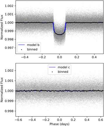
Figure 10. Long- and short-cadence Kepler photometry (gray) phase-folded to the best-fit times of conjunction of planets b (top) and c (bottom). The black points are a running median to more clearly show the transit shape, and the blue curve is the phase-folded model. For planet b, the transit ingress and egress are sharp, with no evidence of horizontal smearing from improperly determined transit times. Transits of planet c are not detected.
Download figure:
Standard image High-resolution image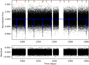
Figure 11. Short-cadence Kepler photometry (black) within the 2σ confidence interval of the expected conjunction of planet d (the maximum likelihood value for which is marked with the yellow notch at the top of the figure). Several transits of planet b (red notches) and non-transiting conjunctions of planet c (green notches) also occur during this time. The best-fit photodynamical model is the blue line. We do not visually detect a transit of planet d in these data.
Download figure:
Standard image High-resolution image5.3. Transit Times
One outcome of the photodynamical modeling is a model-dependent determination of the individual transit times. The transit midpoint times Ti, impact parameters bi, and planet velocities during transit vi and their uncertainties, are given in Table 6 for Kepler-88 b from the date of the first Kepler transit through 2022 November.
Table 6. Kepler-88 b Transit Times and Velocities
| Epoch | Ti | Ti Err. | bi | bi Err. | vi | vi Err. |
|---|---|---|---|---|---|---|
| (BJD−BJD0) | (BJD−BJD0) | (au) | (au) | (au day−1) | (au day−1) | |
| 0 | 55.0801 | 0.0006 | 0.0017 | 0.0002 | 0.0554 | 0.0004 |
| 1 | 66.0069 | 0.0006 | 0.0017 | 0.0002 | 0.0554 | 0.0004 |
| 2 | 76.9294 | 0.0006 | 0.0017 | 0.0002 | 0.0556 | 0.0005 |
| 3 | 87.8535 | 0.0006 | 0.0016 | 0.0002 | 0.0556 | 0.0005 |
| 4 | 98.7724 | 0.0006 | 0.0016 | 0.0002 | 0.0558 | 0.0005 |
| 5 | 109.6940 | 0.0006 | 0.0016 | 0.0002 | 0.0559 | 0.0005 |
Note. Ti refers to the transit midpoint time, bi is the impact parameter, and vi is the planet velocity during the ith transit. BJD0 = 2454900.
Only a portion of this table is shown here to demonstrate its form and content. A machine-readable version of the full table is available.
Download table as: DataTypeset image
6. Results
6.1. Confirmation of a Giant Planet Near a 2:1 Mean-motion Resonance
In both our RV-only and our photodynamical analysis, we confirm the existence of a giant planet at 22.26 days with a mass of 200  . A Lomb–Scargle periodogram of our RVs produces a very strong peak at 22.26 days, with no significant peaks at aliases or harmonics of this period, indicating that 22.26 days is in fact the period of the perturbing giant planet (Figure 12).
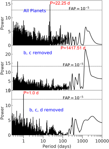
Figure 12. Top: Lomb–Scargle periodogram of the Kepler-88 RVs. Middle: Lomb–Scargle periodogram to the residual RVs, after subtracting the best-fit N-body two-planet model (planets b and c). The significant peak at 1400 days is strong evidence for a third planet in the system. Bottom: Lomb–Scargle periodogram to the residual RVs, after subtracting the best N-body three-planet model. There is a strong peak at 1.0 day that is likely the consequence of correlated noise and our window function. If there is a fourth planet, its orbital period is not yet apparent. The spikes near P = 1 day and higher-frequency harmonics are aliases of the long-period planet(s) and/or long-term RV noise. The false alarm probabilities (FAP) are computed by bootstrap resampling the RVs.
Download figure:
Standard image High-resolution image6.2. Discovery of a Long-period Giant Planet
In the Keck-HIRES RV data, we identify a third planet at  with
with  =
=  . When we compute the Lomb–Scargle periodogram to the residual RVs of a two-planet fit (where the orbits are N-bodies), there is a significant peak at P = 1413 days, and there are no other peaks with comparable power (see Figure 12). We find evidence for the third planet in the significantly improved χ2 statistic to the RVs, which we summarize in Table 4. Without the third planet, our best N-body fit to the TTVs + RVs has
  (see Figure 3). Including the third planet near P = 1413 days results in
  (see Figure 4). The inclusion of the third planet substantially improves the fit to the RVs while simultaneously reducing the HIRES RV jitter by a factor of ∼3. However, the goodness of fit to the TTVs does not change significantly between the two-planet and three-planet models, indicating that the TTVs provide essentially no evidence for the existence of planet d. This is unsurprising, since at
  , the outer planet causes negligible changes to the orbits of the inner planets on the timescale of the Kepler baseline. Therefore, the outer planet was only detected in RVs. The RV-led discovery highlights the importance of multi-method follow-up of the most architecturally interesting Kepler planetary systems.
6.3. Comparison of the RVs Only versus Photodynamical Model
The photodynamical fit provides some advantages over the RVs alone. Although the RV alone identifies the period of planet c as Pc =  days, the photodynamical fit tightens the uncertainty by almost an order of magnitude, finding
  . Note that the precision on our determination of the orbit of planet c is a factor of three better than that of N13, which found
  days; the improvement in the precision of the orbital period must come from the additional Kepler photometry in our analysis, since the RVs alone did not determine the orbit of planet c as precisely as the TTV-based N13 work. Also, the RVs are only able to provide a mass upper limit for planet b, but the planet’s period, radius, and mass are determined with high confidence in the photodynamical analysis:
  (at epoch BJD = 2454954.62702),
  , and
, and  . The superior performance of the photodynamical model for the inner planets illustrates the complementary nature of transit photometry and RVs: together, these techniques reveal more about the 3D architecture of a planetary system than each of these techniques does alone. The superior mass determination of planets b and c in the photodynamical model can be traced to the chopping signal in the TTVs.
6.4. Architectural Constraints from Photodynamical Modeling
From the photodynamical analysis, we determined that the two inner planets, b and c, are apsidally anti-aligned. Our result agrees with N13. Apsidal anti-alignment is a predicted outcome of convergent or divergent Type-I migration in a viscous disk (Nelson 2018, and references therein). The combination of the near-resonant configuration for the inner planets and their apsidal anti-alignment could suggest a history of migration and resonant trapping, although the current anti-alignment is likely a short-lived coincidence (see Figure 9).
Planet d’s longitude of periastron passage is nearly aligned with that of planet b, and anti-aligned with that of planet c. The apsidal alignment of planet d is far less meaningful, since it is dynamically decoupled from the inner two planets. However, the eccentricity of planet d is large ( ) compared to the inner planets (
 ). The high eccentricity of planet d could be explained by planet–planet scattering or Kozai oscillations. By contrast, the modest eccentricities of planets b and c could possibly be explained by the equilibrium of disk and/or tidal circularization and N-body eccentricity pumping.
Because both the inclinations and relative longitude of ascending node are constrained, we can compute the mutual inclination between planets b and c:

We find that the mutual inclination of planets b and c is tightly constrained:  . To test the extent to which the inclinations of the planets are constrained photodynamically, we initialized a DE-MCMC experiment with 40 walkers with our best fit, but flipped the inclination of planet c about the stellar meridian (i = 90°), allowing the same parameters to vary as in our control trial. In general, it is difficult for a DE-MCMC exploration to find this parameter space, because inclinations near 90° for planet c would produce deep transits, which are not observed. However, our inclination-flipped experiment performed substantially worse than our best fit, with ΔBIC = 33 (see Table 4). Therefore, our findings strongly disfavor the model in which planets b and c are on opposite sides of the star; rather, they seem to be on the same side of the star.
Constraints on the mutual inclinations of planets likely come from TDVs. The best-fit solution to our photodynamical model includes substantial TDVs for planet b (see Figure 13), though these are dominated by in-plane eccentricity precession (i.e., Nesvorný et al. 2013). We determined the TDVs based on the velocities and impact parameters in Table 6:

where  is the stellar radius in units of astronomical units, bi is the ith transit impact parameter in units of astronomical units, and
  is the velocity of the planet during the ith transit in units of astronomical units day−1.18
In addition to long-term variation, the TDVs have a chopping signal.
is the velocity of the planet during the ith transit in units of astronomical units day−1.18
In addition to long-term variation, the TDVs have a chopping signal.
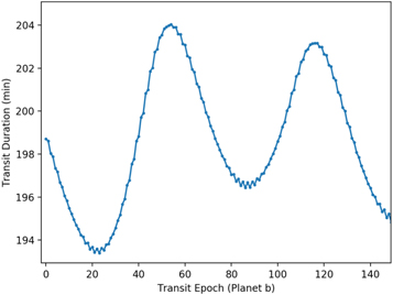
Figure 13. Best-fit durations of the individual transits from our photodynamical model. There are both long-term TDVs and a chopping signal.
Download figure:
Standard image High-resolution imageWe explored the extent to which we could constrain the inclination of planet d from the TTVs. By keeping  constant but varying id and Md, we found that the best-fit solution to the TTVs did not significantly degrade. We tried this experiment in forward modeling the TTVs with TTVFast and also with Phodymm. In both cases, a wide range of mutual inclinations between planet d and the inner planetary system are supported by the data. For example, initializing the inclination of planet d at id = 30° from the sky plane, i.e., about 60° from the inner planets, and thus requiring its mass to be
  , only increased (worsened) the BIC of our photodynamical model by six, which suggests only modestly better performance of a coplanar model. We consider the long-term orbital stability of such solutions in the next subsection. Simulations in similar planetary systems have found that a long-period giant planet is likely to be coplanar with the inner planets, as this configuration is usually stable for longer periods of time than highly mutually inclined geometries (Becker & Adams 2017). In an analysis of the Kepler-88 system, Denham et al. (2019) found that a planet at semimajor axis 2.4 au with
  would be stable so long as its mass was
  . At
. At  , Kepler-88 d could take on a wide range of inclinations without exceeding 20
  and thereby disrupting the inner system.
6.5. Long-term Evolution
The architecture of a long-period giant planet accompanying two closer-in planets reminded us of the Kepler-56 system. Kepler-56 is a red giant star hosting two coplanar, transiting planets whose orbits are misaligned with respect to the stellar rotation axis, which is determined from the asteroseismic modes of the star (Huber et al. 2013). RV monitoring of the system revealed a long-period, non-transiting giant planet with moderate eccentricity (Otor et al. 2016). Follow-up theoretical work (Gratia & Fabrycky 2017) suggested that the outer planet can become eccentric due to planet–planet scattering. In such cases, additional outer planet(s) are likely ejected, leaving the surviving outer planet on an eccentric and inclined orbit. The perturbations ripple to the inner system, not necessarily disrupting it, but possibly causing precession of the orbital plane that periodically misaligns those two planets from the host star’s equatorial plane.19
Here we run a long-term N-body simulation for Kepler-88 to observe the evolution. For the simulation we entered a fit of the data into the Mercury package (Chambers 1999) and used the Burlisch–Stoer integrator for 0.1 Myr to record the secular-timescale effects. We have assumed the outer planet is inclined 30° from our line of sight and ∼27° from the inner planets, but that is not constrained from the data. In Figure 14 we show that no substantial eccentricity is transferred from the outer giant to the inner planets on these timescales, but a long-term precession effect can excite the inner planets to a large inclination from its original plane, and hence relative to the star. The orbital planes of the two inner planets remain closely aligned to each other.
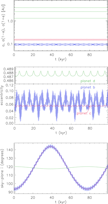
Figure 14. Long-term dynamical simulation of the system. Planets b, c, and d are represented in blue, red, and green, respectively. Top panel: the semimajor axis, periapse distance, and apoapse distance for each planet, as a function of time. Middle panel: planetary eccentricities. Bottom panel: inclination to the sky plane. Over thousands of years, the orbital plane of the inner planets may be torqued through a large angle, away from the transiting configuration. Note that id is unknown.
Download figure:
Standard image High-resolution imageWe follow Boué & Fabrycky (2014) to evaluate the secular timescales. The frequency at which the inner planets would precess due to the outer planet, if the outer planet were not to back-react, is ν3 = 2.7 × 10⁻¹² rad s−1 (74 kyr period). The frequency that the outer planet would precess due to the inner planets, if they were not to back-react, is ν4 = 1.5 × 10⁻¹³ rad s−1 (1.33 Myr period). Together, the frequency of precession should be  rad s−1 (81 kyr period), where Icd is the mutual inclination between planets c and d. The frequencies related to stellar spin precession are several orders of magnitude smaller. Therefore the inner planets are effectively precessing due to the outer planet, without much back-reaction (as is evident also in Figure 14, with a precessional frequency of 77 kyr, near the analytic value), a conclusion that requires only that the outer planet’s angular momentum dominates the system, which is true for any possible inclination of the outer planet. Also, the star’s precession cannot keep up with that relatively quick motion. So we expect that a spin orientation measurement of the star, with respect to the transiting planet’s orbit, would help diagnose whether the outer planet has a significant inclination with respect to the inner planets. For instance, if the spin–orbit misalignment is 20° currently, it is likely cycling between 0° and at least 20°, meaning the inclination of planet d with respect to the inner planets is at least 10°. There may, of course, be more to the dynamics than this simple picture, such as a non-trivial scattering history (Gratia & Fabrycky 2017).
For completeness, we ran two other simulations for 0.1 Myr, one in which planet d is nearly coplanar to the inner system, and one corresponding to the a tilt of 60° and a doubling of the planetary mass as described above. Both simulations remained stable, with quasi-periodic oscillations similar to those in Figure 14. We conclude that planet d does not threaten the stability of the system for a wide range of inclinations.
7. Discussion
7.1. Implications for Planet Formation
Since both planets c and d are gas giants, they must have formed early in the disk lifetime, when gas was abundant. The presence of multiple giant planets in this system is unsurprising since [Fe/H] =  , and the occurrence of giant planets increases with stellar metallicity (Fischer & Valenti 2005). Perhaps additional giant planets were present earlier, or are still present. Planets c and d likely underwent viscous (Type I) migration in the protoplanetary disk. As the gas disk dissipated, planet–planet scattering would likely have increased, and low- and high-eccentricity migration likely became important at this time. The high eccentricity of planet d probably arose due to a significant exchange of angular momentum with another gas giant planet.
The formation of planet b could have been contemporaneous with the giant planets if the planet were somehow gas-starved, resulting in only a low-mass volatile envelope. Or perhaps planet b formed when gas was less abundant and was caught in mean-motion resonance with planet c during an epoch of inward migration of planet c.
7.2. Comparison to Other Planetary Systems
Giant planets are present around a large number of the Kepler systems that host small, transiting planets (Marcy et al. 2014; Mills et al. 2019), and perhaps at greater frequency than giant planets occur around field stars (Zhu & Wu 2018; Bryan et al. 2019). Kepler-88 joins their ranks. Furthermore, Kepler-88 has two giant planets. Other systems with multiple giant planets in addition to small transiting planets include WASP-47 (Neveu-VanMalle et al. 2016) and 55 Cnc (McArthur et al. 2004). The stellar and planetary properties of these systems are summarized in Table 7.
Table 7. Systems with Multiple Giant Planets and Small Transiting Planets
| Parameter | Units | Kepler-88 | 55 Cnc | WASP-47 |
|---|---|---|---|---|
| Stellar Parameters | ||||

|
K | 5466 ± 60 | 5196 ± 24 | 5552 ± 75 |

|

|
0.99 ± 0.024 | 0.905 ± 0.015 | 1.040 ± 0.031 |

|

|
0.897 ± 0.016 | 0.943 ± 0.010 | 1.137 ± 0.013 |
| [Fe/H] | dex | 0.27 ± 0.06 | 0.31 ± 0.04 | 0.38 ± 0.05 |
| Age | Gyr | 1.9 ± 1.6 | 10.2 ± 2.5 | 6.5 ± 2 |
| Innermost Transiting Planet | ||||
| Letter | b | e | e | |
| Period | days | 10.91649 ± 0.00014 | 0.736539 ± 0.000007 | 0.789592 ± 0.000012 |

|

|
3.44 ± 0.08 | 1.91 ± 0.08 | 1.810 ± 0.027 |

|

|
9.5 ± 1.1 | 8.08 ± 0.31 | 6.83 ± 0.66 |

|

|
1.29 ± 0.16 | 6.4 ± 0.8 | 6.35 ± 0.64 |
| Ecc. | 0.05561 ± 0.00013 | 0.040 ± 0.027 | 0.03 ± 0.02 | |
| Innermost Giant Planet | ||||
| Letter | c | b | b | |
| Period | days | 22.2649 ± 0.0007 | 14.65152 ± 0.00015 | 4.1591289 ± 0.0000042 |

|

|
214.0 ± 5.23 | 264.0 ± 1.0 | 363.1 ± 7.3 |
| Ecc. |

|
0.0034 ± 0.0032 | <0.002 | |
| Outermost Known Giant Planet | ||||
| Letter | d | d | c | |
| Period | days | 1403 ± 14 | 4825 ± 39 | 588.5 ± 2.4 |

|

|
965 ± 44 | 1232 ± 22 | 398.2 ± 9.3 |
| Ecc. |

|
0.019 ± 0.013 | 0.296 ± 0.017 | |
Note. For Kepler-88: planetary parameters  and
and  are from this work, and other stellar parameters are from Fulton & Petigura (2018). For 55 Cnc: stellar parameters are from von Braun et al. (2011), and planetary parameters are from Demory et al. (2016, planet e) and Baluev (2015, other planets). For WASP-47: stellar and planetary parameters are from Vanderburg et al. (2017).
Download table as: ASCIITypeset image
Like Kepler-88, WASP-47 has a nearly circular hot Jupiter and a slightly eccentric longer-period giant planet (Sinukoff et al. 2017; Vanderburg et al. 2017; Weiss et al. 2017). Similarly, 55 Cnc has a close-in, nearly circular warm Jupiter at P = 14.7 days, and three other known giant planets at 44.4, 261, and 4800 days (Marcy et al. 2002; McArthur et al. 2004; Naef et al. 2004; Fischer et al. 2008; Wright et al. 2009; Dawson & Fabrycky 2010; Endl et al. 2012; Nelson et al. 2014; Baluev 2015). In general, systems with hot Jupiters do not tend to have companions within ∼1 au (Steffen et al. 2012b), although many such systems have companions from 5 to 20 au (Bryan et al. 2016). Perhaps systems with hot/warm Jupiters in proximity to small exoplanets and/or with metal-rich stars are an exception to these patterns in the broader population. Long-baseline RV studies of the Kepler and Transiting Exoplanet Survey Satellite (TESS) systems with hot and/or warm Jupiters in addition to small planets will reveal whether these systems also have distant giant planets.
Kepler-88 differs from 55 Cnc and WASP-47 in that the innermost known planet has an orbital period of 11 days, rather than <1 day. Both 55 Cnc e and WASP-47 e are examples of ultra-short period (USP) planets, which are defined as having P < 1 day (Dawson & Fabrycky 2010; Becker et al. 2015). USPs are generally small ( ; Sanchis-Ojeda et al. 2014); this is likely because their high equilibrium temperatures do not support a volatile envelope of hydrogen and helium, although they could support thin envelopes of heavier mean-molecular weight species like water or silicates (Lopez 2016). Kepler-88 b is nearly the size of Neptune, and, at a density of 1.1
  , has abundant hydrogen and helium. However, its mass of
  is very similar to the masses of 55 Cnc e and WASP-47 e. We speculate that perhaps the nearby giant planet may eventually perturb Kepler-88 b into an orbit with P < 1 day, where photoevaporation would remove the H/He envelope. One mechanism that could accomplish this rearrangement is that the outer gas giant could perturb the 2:1 resonance to ever-widening libration amplitude, whereupon a scattering interaction between Kepler-88 b and c sends Kepler-88 b on an eccentric orbit which is tidally circularized at a much smaller orbital period. Kepler-88 is significantly younger than the other systems (age = 1.8 ± 1.6 Gyr, see Table 7). Thus, Kepler-88 might represent an early prototype of the 55 Cnc and WASP-47 systems, in particular their inclusion of a hot super-Earth.
7.3. Comparison of RV and TTV Masses
The measurement of planetary masses with RV and transit timing may always be confused by the presence of additional planets perturbing the star (RV) or the transiting planet(s) (TTVs). In addition, both techniques can suffer from stellar systematics such as stellar jitter (RV) or stellar photometric inhomogeneities (TTVs), as well as instrumental systematics. This motivates a comparison of these two techniques when both are available. Unfortunately the number of systems for which this is possible is very small due to the small probability of transit of RV-detected systems, and the poor RV precision of most TTV systems found with Kepler. Mills & Mazeh (2017) found only nine planets which had both RV and TTV mass measurements, of which eight agree to better than 2σ, while one (Kepler-89d) may be influenced by the presence of additional undiagnosed planets (Mayo et al. 2017). Note that each technique has a slightly different dependence upon the stellar mass, so that precise stellar parameters are needed to carry out a comparison.
The Kepler-88 system adds another planet for which both RV and TTV measurements are available: Kepler-88c. In our RV analysis, we found a minimum mass of this planet of  , while in an analysis of the TTVs only using a three-planet model we found a best-fit mass of
  . The photodynamical analysis indicates an inclination for planet c of 93
14, so these two determinations agree to within 1σ. Thus, Kepler-88c adds to the number of cases in which consistent RV and TTV masses are obtained, building confidence in both techniques.
7.4. Opportunities for Future Observation
The presence of two planets in near-resonant orbits can sometimes be confused for a single planet with moderate eccentricity (Wittenmyer et al. 2019). Our RV baseline is too short, and our sampling of the periastron too sparse, to fully explore the possibility of a fourth planet in the system (see Figure 12). Our most recent RV just after the 2020 periastron passage of planet d shows no sign of a fourth planet.
The TESS spacecraft observed Kepler-88 during its northern hemisphere campaign this summer. The photometric precision of TESS should be adequate to detect Kepler-88 b, if the planet is still transiting (Christ et al. 2019).
8. Conclusion
With six years of RV monitoring, we have confirmed the presence, orbit, and mass of the giant planet Kepler-88 c:  ,
,  . This giant planet perturbs the orbit of the transiting planet Kepler-88 b and produces its TTVs. We have also discovered an additional giant planet, Kepler-88 d, in an orbital period of
  with moderate eccentricity of
  and a minimum mass of
  . Our analysis of the RVs only versus a full photodynamical model demonstrated that the RVs were necessary to detect planet d, but that the orbits and masses of planets b and c are much better determined with a full photodynamical model than with RVs alone. Both techniques independently give consistent values for the mass of planet c. Kepler-88 joins the ranks of metal-rich stars that host both small transiting planets and two or more giant planets.
The authors thank the NASA Kepler Science team for providing the exquisite photometry on which this analysis is based. Without the success of the Kepler mission, the observational follow-up presented here would not have occurred.
L.M.W. thanks Molly Kosiarek, Ian Crossfield, Sarah Blunt, Lee Rosenthal, Sam Grunblatt, and Ryan Rubenzahl for contributing to the collection of Keck-HIRES RVs, and Jason Wang, Dan Foreman-Mackey, and Ben Montet for useful discussions.
L.M.W. acknowledges the support of Ken and Gloria Levy, the Trottier Family Foundation, the Beatrice Watson Parrent Fellowship, and NASA ADAP Grant 80NSSC19K0597. D.F. acknowledges support from NASA grant NNX17AB93G. E.A. acknowledges support from NSF grant AST-1615315, NASA grants NNX13AF62G, NNA13AA93A, and 80NSSC18K0829. Kepler was competitively selected as the tenth NASA Discovery mission. Funding for this mission is provided by the NASA Science Mission Directorate. We are grateful to the time assignment committees of the University of California, the University of Hawai`i, and NASA for allocating observing time to complete this multi-year project. This work benefited from the 2017 Exoplanet Summer Program in the Other Worlds Laboratory (OWL) at the University of California, Santa Cruz, a program funded by the Heising-Simons Foundation. This research was partially conducted during the Exostar19 program at the Kavli Institute for Theoretical Physics at UC Santa Barbara, which was supported in part by the National Science Foundation under grant No. NSF PHY-1748958.
The authors wish to recognize and acknowledge the very significant cultural role and reverence that the summit of Maunakea has always had within the indigenous Hawaiian community. We are most fortunate to have the opportunity to conduct observations from this mountain.
Facilities: Kepler - The Kepler Mission, Keck:I (HIRES). -
Software: RadVel (Fulton et al. 2018), TTVFast (Deck et al. 2014), Phodymm (Mills et al. 2016), Rebound (Rein & Tamayo 2016).
Footnotes
- 11
The stellar mass was essentially unchanged, which is the expected behavior from Phodymm (Mills et al. 2016).
- 12
The periods Pb and Pc used in determining the expected chopping signal are from the linear ephemeris (as in Section 3), which are substantially different from the values used in initializing an N-body fit to the TTVs.
- 13
We used the lowest-degree polynomial that removed significant peaks at much longer periods than the expected synodic chopping signal.
- 14
We looked for similar peaks at the other first-order resonances, but only found peaks near j:j − 1 for odd values of j. These peaks also happen to be near the aliases produced by the window function. Further investigation of the full sequence and dynamical origin of the chopping signal periodogram is outside the scope of this paper.
- 15
The longer timescale interactions of planet d are discussed in Section 6.5.
- 16
- 17
We tested this assertion by computing the autocorrelation function of the residuals, the magnitude of which did not exceed 0.002 for lags larger than unity.
- 18
The velocity of the star is ignored here; it is
 the planet velocity.
 - 19
For the Kepler-88 system, another possible consequence could be to leave the resonant libration in an excited state, accounting for the large TTVs.
