Abstract
In this paper, we present the first results from a CARMA high-resolution 12CO(1-0), 13CO(1-0), and C18O(1-0) molecular line survey of the North America and Pelican (NAP) Nebulae. CARMA observations have been combined with single-dish data from the Purple Mountain 13.7 m telescope, to add short spacings and to produce high-dynamic-range images. We find that the molecular gas is predominantly shaped by the W80 H ii bubble, driven by an O star. Several bright rims noted in the observation are probably remnant molecular clouds, heated and stripped by the massive star. Matching these rims in molecular lines and optical images, we construct a model of the three-dimensional structure of the NAP complex. Two groups of molecular clumps/filaments are on the near side of the bubble: one is being pushed toward us, whereas the other is moving toward the bubble. Another group is on the far side of the bubble, and moving away. The young stellar objects in the Gulf region reside in three different clusters, each hosted by a cloud from one of the three molecular clump groups. Although all gas content in the NAP is impacted by feedback from the central O star, some regions show no signs of star formation, while other areas clearly exhibit star formation activity. Additional molecular gas being carved by feedback includes cometary structures in the Pelican Head region, and the boomerang features at the boundary of the Gulf region. The results show that the NAP complex is an ideal place for the study of feedback effects on star formation.
1. Introduction
Feedback from young massive stars is crucial for the evolution of the interstellar media of galaxies. In particular, bubbles driven by young massive stars are common in our Milky Way (Churchwell et al. 2006). They carry momentum and energy, and significantly impact their environments. However, details of these regulatory processes are not well understood, largely because the structure of the gas is often complicated by the effects of multiple massive stars (Dale et al. 2015). Studies of the effects of a single massive star on its natal molecular environment are clearly needed to address this issue.
In this regard, the North America and Pelican (NAP) Nebulae provide a favorable target for investigating the response of a star-forming molecular cloud to a single massive star and its feedback. Within this complex, an H ii region, W80, appears as an ionized bubble at radio wavelengths (Westerhout 1958). The ionizing source is an O3.5 star, 2MASS J20555125+4352246 (Comerón & Pasquali 2005), also known as the Bajamar Star (possibly a spectroscopic binary, cf. Maíz Apellániz et al. 2016).
An optical/near-infrared image of the NAP is shown in Figure 1. A dark cloud, L935, is seen against the bright W80 bubble. The position of the Bajamar Star is indicated by a cyan diamond. The H ii region has been produced by a single massive ionizing source, still embedded in an actively star-forming molecular cloud (Bally et al. 2014, hereafter B14). This is an ideal area for a detailed study of the effects of massive-star feedback on the surrounding environment.
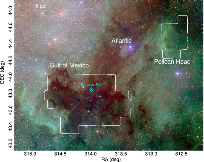
Figure 1. Footprint of the CARMA NAP map (white boundaries) overlaid on a POSS-II false-color RGB image, using the 0.9 μm (Red), 0.7 μm (Green), and 0.43 μm (Blue) bands. The observed regions include the Gulf of Mexico (the dark area to the southeast), and the Pelican Head (the area to the northwest). The cyan diamond marks the position of the O star, as confirmed by Comerón & Pasquali (2005). The cyan arrow points from the O star to the two boomerang features at the southeast corner. The scale bar is derived assuming an 800 pc distance to the NAP complex (Section 4.3).
Download figure:
Standard image High-resolution imageBased on the recent Gaia data, we have learned that the NAP region is about 800 pc away (Zucker et al. 2020, also see Section 4.3). At this distance, a physical scale of 0.1 pc translates to an angular scale of 25″. This scale corresponds to the typical size of star-forming cores and filaments most relevant to star formation studies. To reasonably resolve these structures in the NAP cloud, we have used the Combined Array for Research in Millimeter-wave Astronomy (CARMA) to map emissions from common molecular gas tracers (Section 2.1). The NAP complex is vast, so we limit our maps to regions with predominantly dense gas, i.e., the Gulf of Mexico, and the Pelican Head. These regions are outlined with white boundaries in Figure 1.
CARMA high-resolution molecular line observations are critical for examining the molecular gas/H ii region interactions. However, the analysis of the feedback mechanism also requires an understanding of the effects of a massive star on the overall star formation process. We have therefore complemented our molecular line imaging program with studies of the relationship between the molecular gas and YSOs, using Rebull’s comprehensive YSO catalog (Rebull et al. 2011, hereafter R11).
In this paper, we aim to create a three-dimensional view of the NAP complex by means of a comparison of multi-wavelength images. By pinpointing the interaction between the molecular gas and the H ii region, particularly with respect to the elevated dust emission associated with molecular gas, we aim to distinguish the line-of-sight locations of the molecular gas clouds relative to the H ii region. We also study the number and distribution of YSOs in the associated molecular gas, in order to shed light on how star formation is impacted by the feedback.
2. Observations and Data Combination
As noted above, the NAP region is an example of a relatively simple configuration of a star-forming molecular cloud, a young massive star, and an associated H ii region. The areas of the Gulf of Mexico and Pelican Head mapped by the CARMA observations are shown in Figure 1. These were selected to highlight the most dense gas.
2.1. Observations
CARMA observations were carried out in 2017 during the last season of array operations. The instrument setup was the same as that adopted for the CARMA–NRO Orion Survey (Kong et al. 2018, hereafter K18). Briefly, the 15-element array of six 10 m diameter and nine 6 m antennae was used to map the area of interest. The total mosaicked area of about 1 deg2 is made up of 126 pointings of 6′ × 6′ subfields. The “D”’ and “E” configurations of the array led to uv-coverage between 2.5 and 40 k λ, where λ is 2.6 mm for 12CO(1-0), resulting in an angular resolution of about 7″ (see Table 1).
Table 1. Final Sensitivity
| Transition | Beam | PA | ΔV | σK |
|---|---|---|---|---|
| (deg) | (km s−1) | (K) | ||
| 12CO(1-0) | 7″ × 6″ | 75 | 0.25 | 1.1 |
| 13CO(1-0) | 7″ × 6″ | 75 | 0.16 | 0.8 |
| C18O(1-0) | 7″ × 6″ | 75 | 0.16 | 0.7 |
Download table as: ASCIITypeset image
As for the Orion Survey, the spectral line setup focused on 12CO(1-0), 13CO(1-0), C18O(1-0), but also included the CN N = 1-0, J = 3/2-1/2, SO 2(3)-1(2), and CS(2-1) lines. Here we report only on the 12CO(1-0), 13CO(1-0), and C18O(1-0) observations. With regard to 12CO, the correlator setup provided a bandwidth of 31 MHz (81 km s−1), and a spectral resolution of 98 kHz (∼0.25 km s−1). For the other spectral lines, a bandwidth of 8 MHz (∼21 km s−1) with spectral resolution 24 kHz (∼0.067 km s−1) was used.
To compensate for the fact that the interferometer observations did not include baselines shorter than 2.5 k λ, effectively filtering out emissions from structures larger than 100″, the CARMA observations were combined with single-dish maps of the same regions. These were obtained using the Purple Mountain Observatory Delingha 13.7 m telescope (hereafter DLH14) (Zhang et al. 2014, hereafter Z14), and are part of the Milky Way Imaging Scroll Painting project (Su et al. 2019).
2.2. Data Combination
The CARMA and DLH14 data were combined in the uv plane, following the procedures outlined in Koda et al. (2011), and Kong et al. (2018). The resulting images are based on observations ranging from zero-spacing fluxes to measurements on the maximum baselines provided by CARMA. Figure 2 shows a comparison of CARMA and DLH14 uv sensitivities. The uv-plane pixel sensitivity as a function of baseline length was calculated as per Appendix C in Koda et al. (2011). It is a function of the image-plane sensitivity and the dish size or, for an array, baseline length.
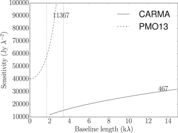
Figure 2. Visibility sensitivity as a function of uv-distance for both DLH14 (dashed curve) and CARMA (solid curve). The imaging sensitivity is labeled next to the curves in units of mJy, as given in Koda et al. (2011). The vertical dotted lines mark the overlapping region between the two data sets.
Download figure:
Standard image High-resolution imageTable 2. Cloud Naming
| Name | R.A. | Decl. | vlsr | Figure |
|---|---|---|---|---|
| (deg) | (deg) | (km s−1) | ||
| F-1 | 313.64623 | 44.09655 | −4.9 | B1 |
| F-2 | 313.31135 | 44.36088 | −2.7 | B2 |
| F-3 | 313.47317 | 44.35101 | 0 | B3 |
| F-4 | 312.99136 | 43.98752 | 3.5 | B5 |
| F-5 | 313.11716 | 43.81911 | 0 | B3 |
| F-6 | 313.32268 | 43.60290 | 0 | B3 |
| F-7 | 314.04069 | 43.57983 | 6.5 | B7 |
| Boomerang1 | 314.43230 | 43.51767 | 1.5 | B4 |
| Boomerang2 | 314.67420 | 43.34278 | 0 | B3 |
| Boomerang3 | 315.10378 | 43.88507 | −2.7 | B2 |
| Boomerang4 | 314.61085 | 43.70758 | 4.9 | B6 |
| Comet1 | 312.62712 | 44.57655 | 2 | 3, 10 |
| Comet2 | 312.60718 | 44.32575 | 0 | 10 |
| Dark Crab | 314.40155 | 43.87826 | 4.9 | B6 |
| Dark Drizzle | 314.46471 | 43.64457 | 4.9 | B6 |
| Dark Filigree 1 | 314.03919 | 43.73130 | 3.5 | B5 |
| Dark Filigree 2 | 314.14630 | 43.66815 | 4.9 | B6 |
| Dark Heron | 313.64063 | 43.73207 | 3.5 | B5 |
| Dark Tail | 313.33844 | 43.46264 | 3.5 | B5 |
| Dark Worm | 314.42482 | 44.07318 | 3.5 | B5 |
| SW-Clump | 314.41301 | 43.73359 | 3.5 | B5 |
Note. F-1, F-2, F-3, F-4 were defined in Z14. Figure 11 shows a summary of the features overlaid on the POSS-II red color image.
Download table as: ASCIITypeset image
In general, to ensure good results in terms of imaging quality when combining observations from two instruments, it is desirable that the sensitivities match where the baselines overlap. Figure 2 shows that this is not the case here; the sensitivity of the DLH14 data is much lower that that of CARMA. The sensitivity mismatch also affects flux-scale determination adversely. As described in Kong et al. (2018), the relative fluxes of the single-dish and CARMA data can be calibrated based on the flux ratio within the overlapping baselines. Here, the DLH14 data is sufficiently noisy, beyond baselines of 2 k λ, that no meaningful flux-scale factor can be established (we therefore adopt the factor of 1). Nevertheless, as we demonstrate below, the DLH14 observations make a useful contribution to our final images, in spite of their quantitative issues. Table 1 summarizes the final sensitivity for the combined data. To match the single-dish observations, a spectral resolution of 0.16 km s−1 was adopted for the combined 13CO and C18O data set.
2.3. Image Quality
To allay concerns about the reliability of the NAP images that result from combining CARMA and DLH14 observations, we compare 12CO integrated-intensity images of the Pelican Head region from DLH14, CARMA, and combined CARMA+DHL14 data. The Pelican Head area was selected, since it appears to encompass multi-scale structures (see Figure 3). The DLH14 map (left panel) shows smooth, extended emission with very little structure, while the CARMA map (middle panel) is irregular, showing the distinct (sharp) edges of the cometary-like cloud in this region. The combined image (right panel) clearly displays the usefulness of adding short-spacing flux information; considerably more of the structure appears to be present, both at the edges and in the body of the cloud.
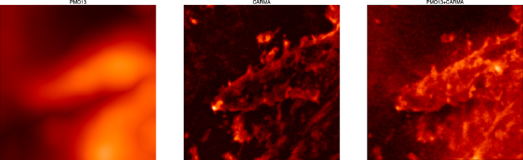
Figure 3. Comparison between DLH14, CARMA, and combined images. Left: DLH14 peak-intensity image. Middle: CARMA image. Right: combined CARMA+DLH14 images. All panels show the same 6′ by 6′ (1.4 pc by 1.4 pc) area, centered around Comet1.
Download figure:
Standard image High-resolution imageIn line with the CARMA–NRO Orion Survey (K18), we carry out a Δ-variance analysis (Stutzki et al. 1998; Ossenkopf et al. 2008) for the channel maps and integrated-intensity maps, so as to examine the quality of the data combination. All main features are visible in the integrated-intensity maps. Figure 4 shows the Δ-variance spectra for the Pelican Head (left panel), and the Gulf of Mexico (right panel) regions. In both regions, and for all tracers, there is a structural break at a scale of 1′–2′, corresponding to the gap in our spatial sensitivity at 1.7–3.4kλ, due to the lack of sensitivity at these scales (see Figure 2). The dip in the Δ-variance at that scale also reflects the mismatch of sensitivity in the overlapping baseline lengths.
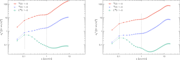
Figure 4. Δ-variance spectra for the 12CO(1-0), 13CO(1-0), and C18O(1-0) integrated-intensity maps from the combined (CARMA+DLH14) data set. The x-axis shows the scale, measured by the wavelet size. The y-axis displays the variance of the structural fluctuations in the maps at that scale, in units of the square of the measured map. The left figure shows the results for the Pelican Head region, the right figure for the Gulf of Mexico. The vertical dotted lines show the scales of the CARMA beam (∼6″), and the DLH14 beam (∼60″).
Download figure:
Standard image High-resolution image3. Results
3.1. Feedback Features in IR and the Ionizing Source
Figure 5 shows a composite image of the Gulf of Mexico and Pelican regions (the same area shown in Figure 1) compiled using Spitzer data at 24 μm (red), 8 μm (green), and 4.5 μm (blue). Figure A1 shows a Wide-field Infrared Survey Explorer (WISE) three-color composite image of the same region, in which we assigned red for the 22 μm emission, green for the 12 μm emission, and blue for the 4.6 μm emission. As in Figure 1, We indicate the extent of the CARMA maps with white boundaries.
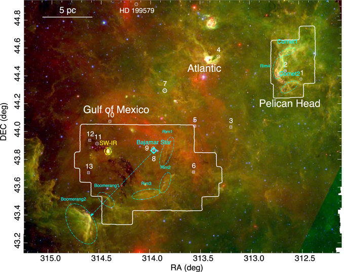
Figure 5. Spitzer false-color RGB image, compiled using the MIPS 24 μm band (Red), and the IRAC 8 μm (Green), and 4.5 μm (Blue) bands. The images are results from Spitzer program 20015, and program 462 (PI: L. Rebull, see R11). The cyan diamond marks the position of the Bajamar Star. The cyan arrow points southeast from the Bajamar Star to the bright-rim feature with a boomerang-like morphology. The cyan dashed ellipses mark several feedback features discussed in the text (and seen in molecular gas in Figures 6 and 8). The white boundaries show the footprint of the CARMA NAP map. Stars numbered 1–13 are from SL08 (as shown in B14). Circles denote stars classified as spectral type OB. Squares are possible AGB stars (see SL08 and B14). The Bajamar Star is #8.
Download figure:
Standard image High-resolution imageIn both Spitzer and WISE images, the Gulf region shows a few relatively bright-rim structures. These bright rims trace hot dust in the area. For instance, the WISE W4 band (22 μm) traces the warm dust thermal radiation. Meanwhile, the WISE W3 band (12 μm) includes many emission features from PAH (at 7.7 μm, 8.5 μm, 10 μm, and 11.3 μm), and fine-structure lines from [Ne ii] (12.8 μm) and [Ne iii] (15.6 μm). These lines are probably pumped by UV emission (Allamandola et al. 1989), and are believed to be good indicators of star formation and stellar feedback (e.g., Ho & Keto 2007). In any case, the hot dust should be heated by a nearby ionizing source.
Here, we argue that the ionizing source responsible for the bright rims seen in these IR images is the Bajamar Star, simply due to the proximity of this high-mass, UV-irradiating young star to these features. As we show in Section 3.2, the labeled bright rims inside the CARMA map area have clear molecular line counterparts. They provide the key connection between molecular gas and massive-star feedback. Hereafter, we designate the bright-rim filamentary structures west and south of the Bajamar Star as Rim1, Rim2, and Rim3, and the bright-rim structures with a boomerang-like morphology to the southeast of the Bajamar Star as Boomerang1 and Boomerang2. There are a few more bright-rim structures in the infrared images which we do not label, as they are either less prominent, or do not have molecular line counterparts.
The morphology of the bright-rim structures can also be used to deduce that the Bajamar Star is the most likely source of feedback in this region. A line passing through the centers of the two boomerang structures and extending to the northwest also passes through the position of the Bajamar Star (see the cyan arrow in Figures 1 and 5). There are two more arc-like features to the northeast of Boomerang2. These features, which are not as bright as Boomerang2, point toward the general direction of the Bajamar Star (see Figures 1 and 5).
As stated above, there is evidence that the Bajamar Star is the main ionizing source in the Gulf region. Straižys & Laugalys (2008, hereafter SL08) reported 12 additional massive-star candidates in the NAP. We determined the distances to these massive stars (including the Bajamar Star) based on the Gaia DR2 results (Bailer-Jones et al. 2018). The Bajamar Star (star #8 in SL08) has a distance of  pc. However, updated results based on Gaia EDR3 find a distance to the Bajamar’s star of d = 785 ± 16 pc, in excellent agreement with the 3D dust and YSO-based results discussed in Section 4.3 of this work. The IRS4 source (star #2 in SL08) in the Pelican region (Bally & Scoville 1980) has a distance of
  pc. However, SL08 suspected that IRS4 is a carbon star. All other candidates are beyond 1500 pc, and there are two sources with no Gaia distances (star #11 in SL08, a.k.a, 2MASS J20580673+4355141; and star #12 in SL08, a.k.a. 2MASS J20582424+4356386). As shown in Figure 1 of B14, these two sources are far to the east of the Bajamar Star. Given the alignment between the Bajamar Star and the bright-rim features discussed above, the Bajamar Star is the only likely massive star responsible for these feedback features in the Gulf region.
We further argue that the Bajamar Star is also the main ionizing star impacting the Pelican region, as suggested by Damiani et al. (2017). The Pelican Head region is clearly being impacted by UV radiation. In Figures 5 and A1 we notice that the Pelican Head region has very bright infrared emission (mostly notable at λ ≳ 5 μm, i.e., visible in IRAC band 3 at 5.7 μm, but barely noticeable in WISE band 2 at 4.6 μm). The same region also exhibits plenty of H2 fluorescent emission, caused by UV emission (as reported by B14), which matches well with the infrared filaments here. In addition, as we discuss in Section 3.2, there are two bright emission features with a comet-like (i.e., head-tail) morphology in the Pelican Head region which were very likely caused by feedback from a massive ionizing star, and which point in the general direction of the Bajamar Star. Hereafter, we therefore assume that all feedback features in this area are the result of feedback from the Bajamar Star.
3.2. Gas Distribution
As can be seen in the 12CO and 13CO 0th-moment maps of the Gulf region (Figures 6(d) and (e)), molecular gas is present over practically the entire area. The only notable decrease in emission occurs toward the southeast corner (near the Boomerang1 structure), and toward the northern-central edge of the map. There are also a number of bright prominent regions throughout the maps. These can be seen more clearly in the peak-intensity maps shown in Figures 6(a) and (b), and discussed below. In contrast, the C18O emission is concentrated in the central-eastern part of the map (Figures 6(c) and (f)). This emission, as discussed below, coincides with the denser parts of the cloud, where 1.1 mm dust-continuum emission has been detected.
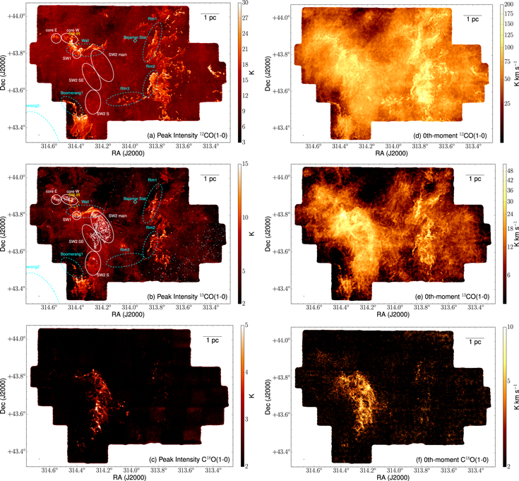
Figure 6. (a): 12CO peak-intensity map for the Gulf region. The synthesized beam is at the lower-left corner. The white ellipses are the BGPS cores defined in B14. The cyan ellipses are as given in Figure 5. (b): 13CO peak-intensity map for the Gulf region. The white contours show the BGPS 1.1 mm continuum, starting from 0.4 Jy beam−1, and increasing in steps of 0.5 Jy beam−1. (c): C18O peak-intensity map for the Gulf region. (d): 12CO 0th-moment map for the Gulf region. The synthesized beam is at the lower-left corner. (e): 13CO 0th-moment map for the Gulf region. (f): C18O 0th-moment map for the Gulf region.
Download figure:
Standard image High-resolution imageFigures 6(a)–(c) show the peak-intensity maps of 12CO(1-0), 13CO(1-0), and C18O(1-0) for the Gulf region. We overlay the Bolocam Galactic Plane Survey (BGPS) 1.1 mm continuum emission (Ginsburg et al. 2013), denoted by white contours. In the Gulf region, the figures show a group of six prominent continuum sources toward the east side of the maps. These are all part of the group of cores traced in 1.1 mm continuum emission, and labeled as “Gulf total” by B14. This includes the two cores designated “Core E” and “Core W” in the northeast part of the map. South of Core W lies the “SW1” core, and toward the southwest of SW1 (from north to south) lie the “SW2 main,” “SW2 SE,” and “SW2 S” cores (B14). These latter three (i.e., the SW2 cores) have prominent C18O counterparts (Figure 6(c)).
There are various prominent features of bright molecular line emission in the Gulf region. Between continuum cores W and SW2 main lies a region of high 12CO and 13CO emission, primarily extending from east to west, which we call the “Wall” (see Figure 6(a) and (b)). It is likely that the Wall, which is at least twice as bright as the average emission in the rest of the map, traces the warm gas heated by a young star lying just north of this structure, which is also responsible for the bright IR nebulosity (hereafter SW-IR) seen in Figures 5 and A1.
Additional prominent line emission regions can be seen in the southeast corner and the mid-western part of the map. In the southeast, the bright emission is coincident with the Boomerang1 feature discussed above (see Section 3.1 and Figure 5). In the central-western region of the map, the bright emission is associated with the IR features labeled Rim1, Rim2, and Rim3 (see Figure 5 and Section 3.1). These, in general, show a sharp increase in intensity toward the edge of the emission structure facing the Bajamar Star (aligning with the IR bright rims defined in Section 3.1 and Figure 5), and have a chaotic morphology in 12CO (Figure 6(a)) and 13CO (Figure 6(b)) away from these bright rims. As discussed later in this paper, these structures are part of the filament F-1, as defined in the study by Z14.
In Figure 7 we show a three-color image comparing the WISE 12 μm band, the peak-intensity map of 13CO, and the peak-intensity map of 12CO. It is very clear that the bright-rim features in the IR image are associated with the bright filaments in molecular line emission. Rim3 overlaps with ripple-like features in CO emission. Moreover, the entire molecular gas structure connected with the rims appears as shredded pieces. A plausible explanation for this is that the expanding bubble has reached (or is very close to) the molecular gas associated with these structures, and the gas therefore exhibits this chaotic morphology because it is being dispersed by the UV photons from the massive star.
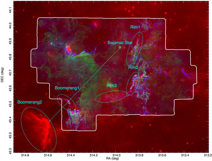
Figure 7. RGB false-color image including the WISE 12 μm band (red), the peak-intensity map of 13CO(1-0) (green), and the peak-intensity map of 12CO(1-0) (blue). The cyan ellipses mark the locations of the feedback features in Figure 5. These match well with the thin CO filaments in the region covered by our CARMA observations.
Download figure:
Standard image High-resolution imageIn the Pelican Head region, we detect 12CO (Figures 8(a) and (d)) throughout most of the mapped area, following a morphology roughly similar to the structure delineated by the yellow-colored features in the Spitzer and WISE three-color composite images. The 12CO, 13CO, and C18O integrated-intensity maps (Figures 8(d)–(f)) show three separate regions of relatively high-intensity emission: in the north (around decl. 4458), center (around decl. 4443), and south (around decl. 443), respectively. These structures are also clearly shown in the peak-intensity maps (Figures 8(a)–(c)). The northern and southern high-intensity regions (which we name Comet1 and Comet2, respectively) have comet-like structures, with bright narrow heads, and with tails extending to the northwest. The central high-intensity structure (which we name Rim4) has a wide arc-like edge and extended (bright) emission to the west, somewhat similar to the Rim2 structure in the Gulf region. All these features roughly point toward the Bajamar Star, and are thus very likely caused by feedback from the massive star.
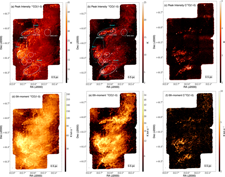
Figure 8. (a): 12CO peak-intensity map for the Pelican region. The synthesized beam is located in the lower-left corner. The white ellipses are the BGPS cores defined in B14. The cyan ellipses are as given in Figure 5. (b): 13CO peak-intensity map for the Pelican region. The white contours show the BGPS 1.1 mm continuum, starting from 0.4 Jy beam−1 and increasing in steps of 0.5 Jy beam−1. (c): C18O peak-intensity map for the Pelican region. (d): 12CO 0th-moment map for the Pelican region. The synthesized beam is located in the lower-left corner. (e): 13CO 0th-moment map for the Pelican region. (f): C18O 0th-moment map for the Pelican region.
Download figure:
Standard image High-resolution imageComet1 is shown in detail in Figure 3. The CARMA high-resolution data shows some ripples at the boundaries of Comet1 (particularly at the northern boundary). Interestingly, both cometary clouds have BGPS sources at their head location, reminiscent of triggered star formation by radiatively driven implosion (Bertoldi 1989). The northern one corresponds to the “Pelican MHO 3402” core in B14 (Figure 3, Table 4), while the southern one corresponds to the “Pelican 8” core in B14.
3.3. Gas Kinematics
Figures 9(a)–(c) show intensity-weighted average velocity (1st-moment) maps of the Gulf region. These provide a general picture of the complex kinematics in this region. In the 12CO and 13CO 1st-moment maps (Figures 9(a) and (b)), the molecular gas associated with the IR bright rims (i.e., Rim1, Rim2) can be seen as gas with average velocities of about −5 km s−1, in sharp contrast with adjacent gas at more redshifted velocities.
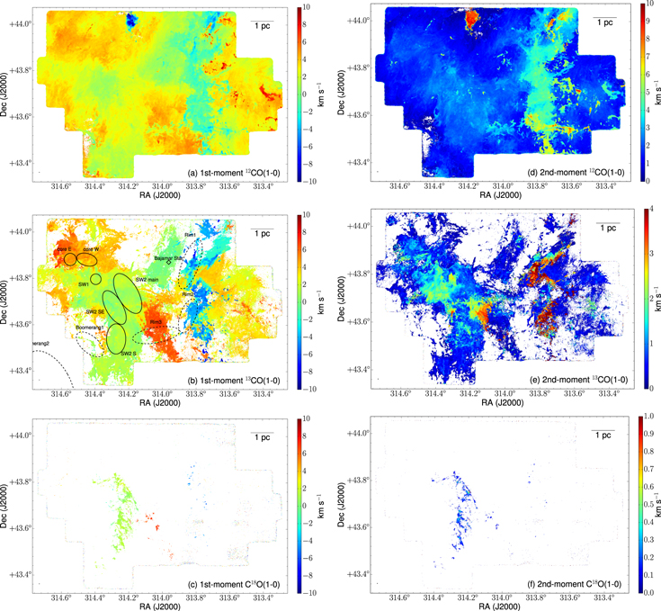
Figure 9. (a): 12CO 1st-moment map for the Gulf region. The synthesized beam is at the lower-left corner. (b): 13CO 1st-moment map for the Gulf region. The ellipses with black solid lines are the BGPS cores defined in B14. The dashed ellipses are the same as the cyan ellipses given in Figure 5. (c): C18O 1st-moment map for the Gulf region. (d): 12CO 2nd-moment map for the Gulf region. The synthesized beam is at the lower-left corner. (e): 13CO 2nd-moment map for the Gulf region. (f): C18O 2nd-moment map for the Gulf region.
Download figure:
Standard image High-resolution imageIn contrast to the Gulf region, the Pelican Head region (Figures 10(a)–(c)) shows a significantly narrower range of intensity-weighted average velocities. Here, most of the emission is concentrated at velocities between −2 and 2 km s−1. In the 13CO 1st-moment map (Figure 10(b)), Comet1 is discernible as an oval region with velocities around 2 km s−1. Comet2 and Rim4 structures are not as conspicuous as Comet1, but are similar to the other feedback features in the NAP, in that the gas beyond the sharp edge is at redshifted velocities, as compared to the feedback structure.
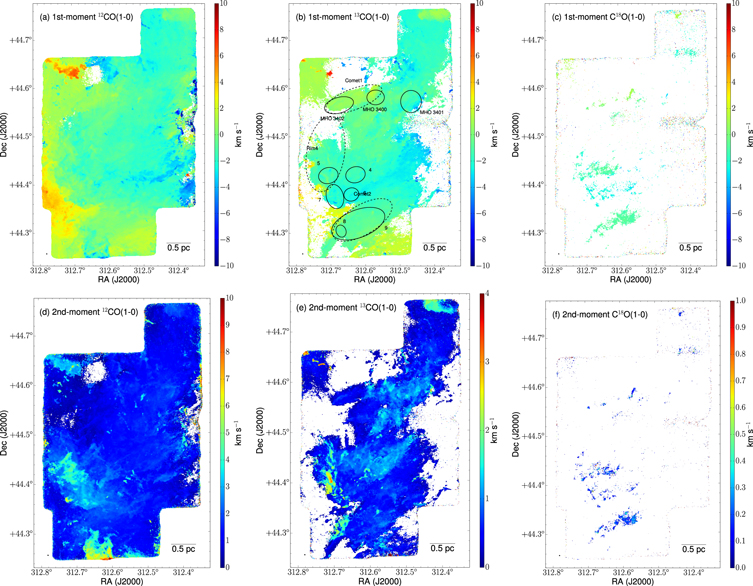
Figure 10. (a): 12CO 1st-moment map for the Pelican region. The synthesized beam is at the lower-left corner. (b): 13CO 1st-moment map for the Pelican region. The ellipses with black solid lines are the BGPS cores defined in B14. The dashed ellipses are the same as the cyan ellipses given in Figure 5. (c): C18O 1st-moment map for the Pelican region. (d): 12CO 2nd-moment map for the Pelican region. The synthesized beam is at the lower-left corner. (e): 13CO 2nd-moment map for the Pelican region. (f): C18O 2nd-moment map for the Pelican region.
Download figure:
Standard image High-resolution imageFigures 9(d)–(f) show 2nd-moment maps of the Gulf region. In the 12CO and 13CO maps (Figures 9(d) and (e)), the gas associated with the bright rims shows large velocity dispersion. On the other hand, the C18O gas (Figure 9(f)) has narrow velocity widths, in sharp contrast with the 12CO and 13CO gas. Figures 10(d)–(f) show 2nd-moment maps of the Pelican region. The gas facing the Bajamar Star exhibits larger velocity dispersion. The gas behind this front is more quiescent. Interestingly, Comet1 does not show large dispersion in either 12CO or 13CO maps.
3.4. Gas Structures Around W80
The moment maps by themselves are not sufficient to permit differentiation between the different cloud components. The distribution of dark patches in the optical image of the region, in conjunction with the location and kinematics of the molecular gas, can be used to derive an approximate three-dimensional distribution of the gaseous structures observed in our map.
The dark patches in the optical image of the NAP in Figure 1, particularly those in the Gulf and Atlantic regions, have generally been thought to be caused by molecular clouds in front of the H ii region, mostly at the same distance (B14, Z14). However, a closer look at Figure 1 suggests a more complicated story. The dark clouds in this image show at least two shades of darkness. One is a semi-transparent gray silhouette, running from the top-right (northwest) edge of the figure throughout the Atlantic area, extending south of the Bajamar Star.
A large area southeast of the Bajamar Star also shows this semi-transparent grayish hue. We designate areas with this shade as “gray regions.” In Figure 1, we also see a collection of patchy clumps that are much more opaque than the gray regions, and which traverse from east to west across the entire Gulf region. We name these areas “dark regions.” These two different shades, combined with information from images at other wavelengths (together with the gas kinematics), imply that there may be more than one group of molecular gases (possibly at different distances) along the line of sight, consistent with our inferences based on the kinematics information. Determining the relation between these two groups of clouds is important in terms of identifying the molecular gas responsible for the star formation taking place in this region, and of understanding the impact of feedback on the molecular clouds in the NAP.
In Appendix B and Figures B1–B7, we identify distinctive, coherent features in the 13CO position–position–velocity (PPV) cube, and compare the gas distribution with different features depicted in the POSS-II red color plate. Figure 11 summarizes the major structures defined, based on this comparison.
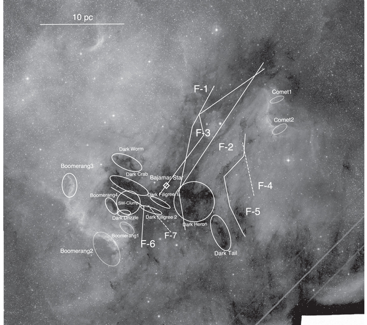
Figure 11. Definition of molecular gas filaments and clumps based on a comparison of POSS-II red color (0.7 μm) and 13CO(1-0) cubes (Section 3.4, Appendix B, Table 2). Background: POSS-II red color plate. The regions mark the filaments and clumps defined in Section 3.4 and Appendix B. The filaments with solid lines are in the foreground. Those with dashed lines are behind the bubble. Filaments F-1, F-2, F-3, and F-4 are as defined in Z14.
Download figure:
Standard image High-resolution image4. Three-dimensional Structure
The most useful information to be gained from the small-scale structures (captured by CARMA) is their morphology matching with the bright infrared rims. The matching between F-1 and the rims confirms that the rims are part of the molecular filament. This finding shows that the filament is being heated and dispersed by the massive star. The morphology match between the molecular filament and the gray regions in the POSS-II image therefore reveal that the gray regions in the optical images probably trace foreground molecular gas that is being destroyed by the Bajamar Star, and is therefore very close to the expanding bubble. As a result of this, the three-dimensional picture of the entire NAP becomes clearer.
4.1. Three-dimensional Structure of the NAP Complex
Figure 12 shows a schematic of the line-of-sight structure of the NAP complex. The locations are given in a relative sense, and are based on the findings discussed in Section 3.4 and Appendix B. We include the major structures defined in Appendix B. These structures occur mainly in the Gulf and Atlantic regions, with a few in the Pelican region and behind the W80 bubble.
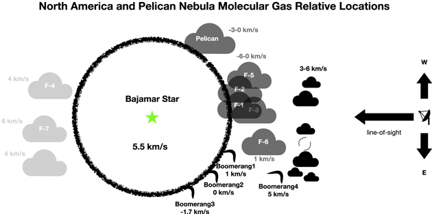
Figure 12. Line-of-sight locations of filaments and clumps relative to the W80 bubble (black circle). The Bajamar Star is at the center of the bubble. Three groups of clouds are shown, including the far-side clouds (F-4, F-7, and another clump to the northeast of the Gulf region, see Section 3.4 and Figure B5), the foreground-contacting gray clouds, and the foreground dark clumps and filigrees (closest to the observer). The LSR velocities of the clouds are also included. We assign a velocity of 5.5 km s−1 to W80, based on the radio recombination line observation by Lockman (1989).
Download figure:
Standard image High-resolution imageThere are three major groups of clumps and filaments, based on their line-of-sight distance. The closest to us comprises a group of dark clumps of varying morphologies (see Figure 11 and the rightmost dark structures in Figure 12). These are in front of the W80 bubble, and appear as dark shadows in the POSS-II images. The group members are small and clumpy, with many ∼10,000 au globules. Their Vlsr is similar to that of the bubble.
Between the dark group and the W80 bubble is the group of gray clouds. F-1 is very close to the bubble, being part of this group; it is lit in the mid-to-far-infrared, and shows bright rims (Section 3.4 and Figures 5, A1, 6, B1). F-2, F-3, and F-5 are also close to the bubble, particularly in the Atlantic region, based on their similar extinction and velocity to the F-1 filament. F-6 may not be so close to the bubble as F-1, but it is between the bubble and the Dark Crab. Boomerang1 and Boomerang4 appear to be dark in the optical image. They are located on the near side of the bubble. Boomerang2 and Boomerang3 are probably on the edge of the expanding bubble.
Behind the bubble are several background clumps, including F-4 and F-7. These do not show gray/dark counterparts in the optical images, and are moving away at ∼5 km s−1. It is not clear whether they are close to the bubble. We suspect that F-7 (covered by our CARMA observations) is not very close to the H ii region, as it does not exhibit the “shredded” and chaotic structure of F-1.
4.2. Correlation between Gas and Extinction
As an independent approach to associate the different velocity components to structures seen in the optical image as foreground layers, we correlate the 13CO data with the foreground extinction. We focus on the combined data in the Gulf region. Instead of using existing extinction maps that trace the whole column of material (e.g., Cambrésy et al. 2002), we obtain an approximate foreground extinction map from the POSS-II red image in Figure 11 by assuming that the highest intensity in the region represents the typical radiation from the bubble, and translating all lower intensities into an an effective red extinction. The resulting foreground extinction map is shown in the top left panel of Figure 13.
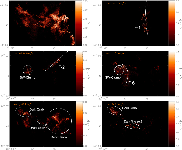
Figure 13. Maps showing the correlation between optical extinction and 13CO emission. Top left: map of foreground extinction, based on the POSS-II red image in Figure 11. Other panels: covariance maps of the foreground, with selected 13CO velocity channels. The velocity is labeled in the top left corners.
Download figure:
Standard image High-resolution imageWe investigate the correlation between 13CO gas and extinction by computing the covariance between the optical image and the 13CO channel maps. 19 For the 13CO channel covariance maps (shown in 13), only noise contributions above 4σ were considered.
We find a strong correlation around −5 km s−1 (the channel including F-1, Figure B1), −2 km s−1 (including F-2, Figure B2), and 4 km s−1 (including SW-Clump, Dark Filigree 1, Dark Heron, Figure B5). At 1.3 km s−1 (including F-6, Figure B4) and 6.4 km s−1 (including Dark Crab, F-7, Figure B7), we actually find a significantly weaker correlation, due to additional emission at those velocities, stemming from the background. Most importantly, the calculation suggests that the Dark Crab is a itself a structure, distinct from the F-6 filament. Although it appears at the same velocity as the F-7 gas, both its dark appearance at near-infrared wavelengths and its well-resolved structure indicate that it must represent material in front of the bubble, closer to us. This is important in terms of being able to match known YSO clusters in the NAP region with their host molecular gas (see Section 5.1). Of particular interest is the SW-Clump, which seems to have counterparts at −2 and 4 km s−1. In the molecular line cubes of 12CO and 13CO, we find that this clump actually spans a wide velocity range, encompassing the velocity of the F-6 filament. The average spectrum of the SW-Clump shows two peaks at about −2 and 4 km s−1. A possible explanation for this is that the clump is elongated along the line of sight, with its far side being pushed by the bubble to produce the negative velocity component. The SW-Clump is likely to be connected or associated with the F-6 filament.
4.3. Distance to the NAP Region
In this section, we discuss the distance to the NAP based on YSOs, 3D dust mapping, and the presumed ionizing star (Bajamar’s star).
We begin by utilizing the Gaia distances (Bailer-Jones et al. 2018) of YSOs associated with dark clouds in this region to evaluate the distance to the NAP region. Figure 14 shows an overview of the YSOs in the NAP region from R11. This YSO classification was based on the near- to mid-IR spectral slope (from 2 to 24 μm, see Section 5.2 of R11). 20 We cross-matched each of the 2000-plus sources in the catalog of NAP YSOs produced by R11 with the Gaia distance catalog (Bailer-Jones et al. 2018), using a search radius of 2″, finding that just over 1000 sources have Gaia measurements.
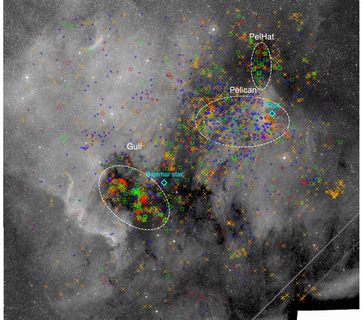
Figure 14. Distribution of young stellar objects in the NAP region. Grayscale background: POSS-II red band image from Figure 1. YSOs from R11 are given by different symbols: red circle—Class I, green box—Class flat, blue arrow—Class II, purple cross—Class III, orange “x”—unknown. The three white dashed circles mark the locations of the clusters (Gulf, Pelican, PelHat), as defined by R11.
Download figure:
Standard image High-resolution imageIn Figure 15, we show a histogram of Gaia distances for all the R11 YSOs available in the Gaia catalog. We zoom in to a range of distances between 0 and 1500 pc, as sources beyond 1500 pc are highly unlikely to be associated with the NAP complex. As shown in the histogram, there is clearly a peak around 800 pc (there is a tail extending from 1500 pc to about 7000 pc, but no other peaks). Assuming that the YSOs are close to, or associated with, the molecular gas in the NAP complex, then the histogram implies that these clouds are located at a probable distance of ∼800 pc. Recently, Zucker et al. (2020) reported a similar distance in regard to the NAP region, based on 3D dust mapping. Kuhn et al. (2020) also reached a similar conclusion, based on a more detailed study of stellar components of the NAP region.
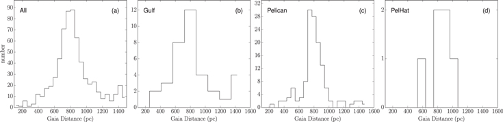
Figure 15. Distribution of (available) Gaia distances to the YSOs, as identified by R11. Panel (a) shows the histogram for all YSOs in the region. Panels (b)–(d) show the distribution of Gaia distance for the three different clusters in the region. The cluster is identified in the top left corner of each panel. The y-axis shows the number of YSOs in each distance bin. Note that we limit the x-axis to distances between 0 and 1500 pc. YSOs beyond 1500 pc are not likely to be associated with the NAP complex.
Download figure:
Standard image High-resolution imageA distance of 800 pc, estimated using the YSOs, is at odds with the original distance from  pc that we derived to Bajamar’s star, based on Gaia DR2 parallax measurements. Even if one considers the upper bound of the uncertainty, the deduced distance would be about 100 pc closer than the distance derived from either YSOs or 3D dust mapping. Fortunately, the higher-precision astrometry and improved treatment of systematic effects available with Gaia EDR3 has resolved the discrepancy in the previous DR2 parallax measurement; Kuhn & Hillenbrand (2020) report a new distance to the Bajamar’s star of 785 ± 16 pc.
In panels (b)–(d) of Figure 15, we separately plot the distance histogram for the three clusters defined in R11. Their names are Gulf, Pelican, and PelHat, and we mark their locations with white dashed ellipses in Figure 14. One can see from Figure 15 that all three YSO clusters peak at ∼800 pc. The PelHat cluster has a limited number of members, so its distance is uncertain. However, the Gulf cluster, which is associated with the foreground gray/dark features (Dark Crab and F-6, see Section 5.1), also has a peak distance of ∼800 pc. Since the W80 region is behind the gray/dark features, the distance to the W80 region must be farther than the Gulf cluster. While this contradicts the Gaia DR2 distance measurement for the Bajamar Star, it is entirely consistent with the more accurate Gaia EDR3 measurement (see Kuhn & Hillenbrand 2020).
We have produced an interactive distance map of the NAP, based on 3D dust mapping (available here), following the technique outlined in Zucker et al. (2019, 2020). Figure 16 shows the distribution of dust along the line of sight toward three representative subregions (≈1 deg2 in area) of the map, centered at (l = 840, b = −18), (l = 844, b = 03), and (l = 851, b = −03), respectively. Similar region-by-region plots over the full cloud are available online. The distance uncertainties for the nebula do not include any systematic uncertainties, which we estimate to be 5% in distance.
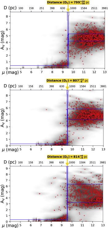
Figure 16. The distribution of dust extinction AV as a function of distance modulus μ (or distance D) for three subregions of the NAP (≈1 deg2 in area), centered on (l = 840, b = −18) (top), (l = 844, b = 03) (middle), and (l = 851, b = −03) (bottom). The blue line shows the infrared distribution of dust along the line of sight for each subregion. In each panel, a sharp increase in extinction (marked with a yellow arrow) indicates the most likely distance to that subregion of the NAP. The red crosses indicate the most likely distance and integrated dust extinction for stars toward each subregion, which are collectively used to constrain the dust distribution. Based on similar analyses across the full NAP region, we infer an average distance to the cloud of 797 ± 40 pc.
Download figure:
Standard image High-resolution imageFor the full map, see https://faun.rc.fas.harvard.edu/czucker/Paper_Figures/NorthAmerica.html. To produce the map, we grid the NAP region into individual pixels (based on the Healpix system, with a resolution parameter (Nside) of 64, Gorski et al. 2005) following Zucker et al. (2019), where each pixel covers about 1 deg2 on the Sky. Each pixel is color-coded according to the distance we infer for the dust in that subregion. We are able to target all areas with an extinction of at least 5 mag. Each subregion is fit independently, with a typical uncertainty of about 5%–6% in distance, or about 40 pc. The distances obtained via 3D dust mapping are complementary to YSO-based distances, obtained either from Gaia DR2, or from VLBI observations (e.g., toward masers; Reid et al. 2019). Zucker et al. (2020) find that their 3D dust-mapping approach agrees with maser distances to within 10% out to 2.5 kpc, with no systematic offset.
While it is difficult to definitively constrain distance gradients within the NAP given our typical systematic uncertainty (≈40 pc), we determine that the entire NAP region traced by dust is consistent with its being at the same distance, to within a few tens of parsecs. Using distance information across the full cloud, we find an average distance of 797 ± 40 pc, in excellent agreement with the Gaia DR2 distances toward YSOs given in Figure 15. Our results are also consistent with the updated distance to Bajamar’s star—the presumed ionizing star—based on recent Gaia EDR3 results (from Kuhn & Hillenbrand 2020), who find that d = 785 ± 16 pc.
On a side note, the Gulf cluster distance histogram in Figure 15 shows a tentative excess at ≲800 pc, while the Pelican cluster shows a clearer excess at ≳800 pc. This distance difference implies that the Gulf cluster has members that are closer to us, which is consistent with the Gulf cluster being associated with a near-side clump/filament. Indeed, Kuhn et al. (2020) reported that stars in the Gulf region (their group E) are ∼35 pc closer than stars in the Atlantic and Pelican regions (their groups A to D at ∼795 pc).
5. Discussion
5.1. Star Formation and Feedback
Out of the three clusters discussed in Section 4.3, and shown in Figure 14, the Pelican cluster does not have a morphological match with molecular gas structures. The Pelican Head region (northwest of the Pelican cluster from R11, and south of the PelHat cluster from R11) has multiple MHOs, as identified in B14, indicating that the young stars there are still accreting from the molecular gas. However, the rest of the Pelican cluster (outside the Pelican Head region) has very limited 13CO(1-0) or C18O(1-0) emission, except for those young stars near the Atlantic region. R11 also noted that the cluster is in a low-extinction region (based on the extinction map of Cambrésy et al. 2002).
Kuhn et al. (2020) noticed that the Pelican cluster (their Group D) shows evidence of expansion. As discussed in Section 3.4, the Atlantic clouds are clearly associated with the bright rims, and are probably being dispersed by the Bajamar Star. A possible scenario is that the molecular gas associated with the Pelican cluster, probably the gas in the Atlantic region, is being dispersed by the massive star. The forming cluster was originally confined by the cloud’s gravitational potential, but is now expanding due to the (sudden) dispersal of the cloud. If true, then the Pelican cluster is a good example of cluster formation being halted by feedback from a nearby massive star. In other words, the cluster formation reaches an end, not because its associated gas is consumed or dispersed by the cluster itself, but by a neighboring massive star.
Here, we carry out a simple analysis to test the possibility that the cloud (hereafter the pre-Pelican cloud) in which the Pelican cluster formed might be being dispersed by the Bajamar Star. We note that the PelHat cluster (north of the Pelican cluster) overlaps with relatively high-extinction regions (see Figure 14). It is located at the edge of the W80 bubble, and has ample molecular gas with which to continue forming stars and feeding the accretion of existing protostars. Indeed, a recent survey of outflows (Zhang et al. 2020) has revealed a few molecular outflows in PelHat, indicating active protostellar accretion. Meanwhile, we know that the Pelican cluster has little molecular gas. It is therefore probable that the pre-Pelican cloud was stripped from the Pelican cluster. Either the pre-Pelican cloud was pushed away by radiation pressure or bubble expansion, or the cloud was ionized by the Bajamar Star. In any case, the Pelican cluster should be closer to the Bajamar Star than PelHat. In other words, the cluster should be inside the bubble by now.
To carry out our basic feedback analysis, we need to estimate and make various assumptions about the H ii region and the pre-Pelican cloud. The ionizing photon flux from the Bajamar Star is SUV ∼ 1049 s−1, and the electron density, ne , of the H ii region is ∼10 cm−3 (Wendker 1968; Comerón & Pasquali 2005). The ionizing flux, S, from the Bajamar Star corresponds to a luminosity of 2.2 × 1039 erg s−1 (assuming 13.6 eV photon energy). The W80 bubble radius is ∼20 pc, much larger than the Strömgren radius of ∼2.8 pc (assuming a mean gas number density, n, of 100 cm−3 before ionization, see Equation (7.24) in Krumholz 2017). Hence, the bubble is likely to have expanded significantly. Assuming a temperature of 104 K for the H ii region, the corresponding sound speed is ∼11 km s−1. If we assume a mean stellar mass of 0.5 M⊙ (Evans et al. 2009) for the Pelican cluster members, then the total cluster mass (with 247 members, R11) is ∼120 M⊙. Assuming a star formation efficiency of 3% (Kennicutt & Evans 2012), the total pre-Pelican cloud mass M would be 4 × 10³ M⊙,
Firstly, we consider that the pre-Pelican cloud was pushed by bubble expansion. Assuming that thermal pressure in the bubble dominates the expansion, then the total expansion time can be computed following Equation (7.32) in Krumholz (2017).

where ri is the radius of the ionized sphere, S49 is the ionizing photon flux (in units of 1049 s−1), n2 is the initial number density before ionization (in units of 100 cm−3), Ti,4 is the temperature of the ionized gas (in units of 104 K), and t6 is the time of expansion (in units of 106 yr). Adopting ri = 20 pc, S49 = 1, n2 = 1, and Ti,4 = 1, the total expansion time, t, is about 3.7 Myr. Taking the time derivative of the equation, the current bubble expansion velocity is

which is about 3 km s−1. The typical relative velocity between the molecular filaments in the NAN region and the W80 bubble is a few km s−1. Bubble expansion is therefore a possible mechanism for the dispersal of the pre-Pelican cloud. Considering the geometry, it is possible that the molecular gas to the northwest of the Pelican Head is partly composed of gas from the pre-Pelican cloud that has been pushed to that position.
Secondly, we consider that the Lyα photons from the H ii region exert a radiation pressure on the molecular gas. Assuming that the solid angle subtended by the pre-Pelican cloud (as viewed from the Bajamar Star) is Ω, then the force caused by the radiation pressure is SΩ/4π c, where c is the speed of light. The final velocity of the pre-Pelican cloud after t is (SΩ/4π c)t/M. If we assume that Ω = 4π/10, the pre-Pelican cloud reaches a velocity of about 1.1 km s−1, smaller than that found for bubble expansion.
Finally, we consider that the pre-Pelican cloud was ionized by the Bajamar Star, so that we do not see the molecular gas today. For an ideal Strömgren sphere, the ionized gas mass is SUV μ mH /n αB , where μ = 1.4 is the mean particle weight, mH is the hydrogen mass, n is the particle density, earlier assumed to be 100 cm−3 (see Equation (7.23) in Krumholz 2017), and αB = 3.5 × 10⁻¹³ cm3 s−1 is the case B recombination coefficient for hydrogen. Given the aforementioned flux, SUV, the H ii region mass is about 3 × 10³ M⊙, comparable to the pre-Pelican cloud mass M.
The actual history of the cloud dispersal may comprise a combination of bubble expansion, radiative pressure, and ionization. In other words, part of the pre-Pelican cloud may have been ionized, and the rest could have been pushed away. In any case, it is possible that the Bajamar Star and the W80 bubble together could have dispersed the pre-Pelican cloud.
5.2. The Gulf Cluster
The Gulf cluster, however, requires closer examination. There are probably three subclusters in this region. From west to east, Guieu et al. (2009, hereafter G09) named them clusters 1, 2, and 3 (see their Figure 9). Based on our combined molecular line data, we find evidence that the three subclusters are probably separated.
In Figure 17, we show the 13CO gas associated with the three G09 subclusters. In panel (c), the G09 cluster 3 is associated with a 24 μm dark region at the northeastern end of the Gulf region (the “Dark Crab”). It is embedded in highly extinct molecular gas at ∼4.9 km s−1. Meanwhile, the G09 cluster 2 spatially matches the 24 μm dark region of the F-6 filament, at a velocity of ∼1.5 km s−1. Consequently, the two G09 clusters are associated with two distinct molecular gas regions. As such, they are probably not part of the same cluster.
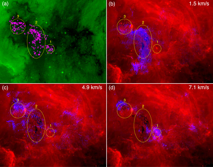
Figure 17. (a): POSS-II red color plate for the Gulf region, given as in Figures B1–B7. The magenta crosses mark the R11 Gulf cluster members. The yellow dashed ellipses mark the G09 subclusters. (b): The background red color shows the Spitzer 24 μm image from R11. The blue color shows the CARMA+DLH14 combined 13CO channel map at 1.5 km s−1. The 24 μm dark regions are partially covered by the blue color. Readers can see these more clearly in Figure 5. (c): As panel (b), but showing the 4.9 km s−1 channel. (d): As panel (b), but showing the 7.1 km s−1 channel.
Download figure:
Standard image High-resolution imageMore interestingly, the location of the G09 cluster 1 has no 24 μm dark counterpart, as shown in Figures 17 (b) and (c). This cluster nicely coincides with the location of the background F-7 filament (Figures 11 and B7). This is especially true at 7.1 km s−1 (panel (d)). It is possible that the G09 cluster 1 is embedded in F-7, which lies on the far side of W80. Six members in cluster 1 have Gaia DR2 data: their distances are (in ascending order) 1103, 1111, 1611, 1863, 2457, and 3565 pc. These distances are significantly larger than the estimated distance to W80, and are therefore consistent with the scenario whereby this is a cluster background to W80.
Overall, we see that at least some of the star formation activity in the NAP complex is strongly impacted by feedback from the Bajamar Star.
6. Summary and Conclusion
We have presented high-resolution CARMA molecular line data toward the North America and Pelican Nebulae. Here, new interferometer data is combined with existing single-dish data from the DLH14 telescope to study the structure and kinematics of the molecular gas in this region. The combined maps show ongoing interaction between the molecular gas and feedback from the massive Bajamar Star (O3.5), which is responsible for the W80 H ii region. The molecular gas is being dispersed by W80.
The high-resolution data reveal the intricate morphology of the gas. A substantial fraction of the clouds have a very clumpy structure with sharp edges. Some of these bright edges coincide with the location of bright infrared rims, which generally point toward the Bajamar Star. We argue that these are heated by the massive star, and that the gas is being dispersed.
Using multi-wavelength data (optical, infrared, and millimeter), we have identified a number of distinct structures in the cloud complex, including a number of dark clouds and globules. We have cross-matched the structures in images at different wavelengths, and determined the relative line-of-sight distances of the molecular filaments and clumps.
We find that there are two groups of molecular clouds between the W80 bubble and us. The first group (“gray regions” in the optical image) contains most of the molecular gas in the region, stretching from the Gulf region in the south to the PelHat region in the north. It is also the main host of the young stellar objects in the Nebulae. However, this group of molecular clouds is being impacted by, and will soon be dispersed by, massive-star feedback. The second group of molecular gases (“dark regions” in the optical image) consists of scattered molecular gas clumps that are less massive. These clumps appear darker in the optical image, indicative of higher extinction in these clumps. They show limited star formation (except for one clump that we call the Dark Crab), and are being approached by the expanding W80 bubble.
To determine the distance to the NAP complex, we obtained the Gaia distances to stars in three young stellar object clusters identified by Rebull et al. (2011). The results show that the majority of the cluster members are located at ∼800 pc, indicating that the NAP complex is located at this distance. We provide an interactive distance map, based on the method developed in Zucker et al. (2019, 2020). The map is consistent with the ∼800 pc NAP distance, and provides further details of the 3D structures of the complex, which are broadly consistent with our conclusions, based on matching the morphology of structures found in optical, infrared, and millimeter molecular line maps of the region.
The PelHat and Gulf clusters defined by Rebull et al. (2011) show a clear association with molecular gas. The third cluster, the Pelican cluster, is associated with substantially less molecular gas. We suggest that the gas in this cluster has been dispersed by the O-type Bajamar Star, not by sources within the Pelican cluster. It seems, therefore, that the star formation in the Pelican cluster has been interrupted by the massive star. The pre-Pelican cloud was probably dispersed by a combination of bubble expansion, radiative pressure, and gas ionization. This scenario provides a good example of feedback-regulated star formation. The North America and Pelican Nebulae therefore provide a nearby example for the study of star formation under the influence of an isolated massive star.
We thank the anonymous referee for the thorough check of this paper, and the helpful comments. We thank Luisa Rebull for providing the Spitzer images. We thank Laurent Cambrésy for providing the extinction maps. S.K. acknowledges fruitful discussions with Min Fang and Serena Kim. S.S. acknowledges support from the European Research Council under the Horizon 2020 Framework Program, via the ERC Consolidator Grant CSF-648505. T.G.S.P. gratefully acknowledges support by the National Science Foundation under grant No. AST-2009842. S.K. and H.G.A. were (partially) funded by the National Science Foundation, award AST-1140063, which also provided partial support for the CARMA operations. The CARMA operations were also supported by the California Institute of Technology, the University of California–Berkeley, the University of Illinois at Urbana-Champaign, the University of Maryland College Park, and the University of Chicago. A.S.M. and V.O. carried out this research within the Collaborative Research Centre 956 (subprojects A6 and C1), funded by the Deutsche Forschungsgemeinschaft (DFG)—project ID 184018867. Part of this research was carried out at the Jet Propulsion Laboratory, California Institute of Technology, under a contract with the National Aeronautics and Space Administration. Contributions from J.K. are in part supported by the National Science Foundation under grant Number AST–1909097. S.Z. acknowledges funding from the National Natural Science Foundation of China, through grant No. NSF 11803091. R.J.S. acknowledges funding from an STFC ERF (grant ST/N00485X/1). R.S.K. acknowledges support from the Deutsche Forschungsgemeinschaft (DFG) via the Collaborative Research Center (SFB 881, Project ID 138713538) “The Milky Way System” (subprojects A1, B1, B2 and B8), and from the Heidelberg cluster of excellence (EXC 2181-390900948) “STRUCTURES: A unifying approach to emergent phenomena in the physical world, mathematics, and complex data,” funded by the German Excellence Strategy. He also expresses thanks for funding from the European Research Council, via the ERC Synergy Grant “ECOGAL—Understanding our Galactic ecosystem: From the disk of the Milky Way to the formation sites of stars and planets” (project ID 855130). This research made use of the data from the Milky Way Imaging Scroll Painting (MWISP) project, which is a multi-line survey in 12CO/13CO/C18O along the northern galactic plane, using the Purple Mountain Observatory Delingha 13.7 m telescope. The MWISP project is supported by the National Key R&D Program of China under grant No. 2017YFA0402700, and the Key Research Program of Frontier Sciences, CAS under grant No. QYZDJ-SSW-SLH047. The Second Palomar Observatory Sky Survey (POSS-II) was conducted by the California Institute of Technology with funding from the National Science Foundation, the National Aeronautics and Space Administration, the National Geographic Society, the Sloan Foundation, the Samuel Oschin Foundation, and the Eastman Kodak Corporation. The Oschin Schmidt Telescope is operated by the California Institute of Technology, and the Palomar Observatory.
Facilities: CARMA - Combined Array for Research in Millimeter-Wave Astronomy, DLH:13.7 m. -
Software: Astropy (Astropy Collaboration et al. 2013), Numpy (van der Walt et al. 2011), APLpy (Robitaille & Bressert 2012), Matplotlib (Hunter 2007).
Appendix A: WISE Image
In Figure A1, we present a WISE RGB color image as a supplement to Figure 5.
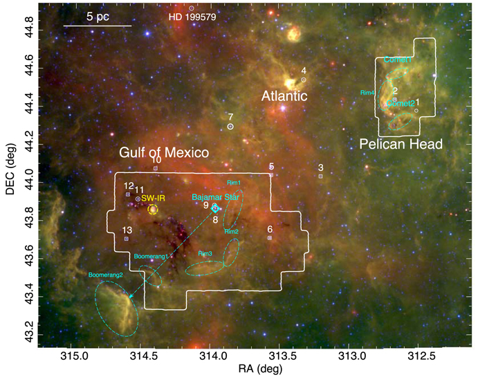
Figure A1. WISE false-color RGB image using the 22 μm (Red), 12 μm (Green), and 4.6 μm (Blue) bands. The cyan diamond marks the position of the Bajamar Star. The cyan arrow points from the Bajamar Star toward the two boomerang features at the southeast corner. The two cometary clouds are seen in molecular gas in Figure 8. Stars numbered 1–13 are from SL08 (as shown in B14). The circles denote stars classified as spectral type OB. Squares indicate possible AGB stars (see SL08 and B14). The Bajamar Star is #8.
Download figure:
Standard image High-resolution imageAppendix B: Structure Identification
Figures B1–B7 show a comparison between the POSS-II red plate and the 13CO(1-0) emission at different velocities. The seven figures have the same four-panel setup, which enables us to compare the gray/dark features in the optical images with the molecular gas distribution at large and small scales. In all panels, the green-colored map shows the POSS-II red plate image. Panels (a) and (b) show the large-scale NAP area (similar to the area shown in the optical and IR images in Figures 1 and 5), while panels (c) and (d) zoom in on the Gulf region. The blue color in panel (b) shows the 13CO(1-0) emission in one channel from the DLH14-only maps. This same emission is represented by blue contour lines in panel (a). The blue color in panel (d) shows the 13CO(1-0) emission from the combined (CARMA+DLH14) cube at the same velocity (Vlsr) as the emission shown in panels (a) and (b).
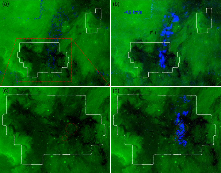
Figure B1. Comparison between the POSS-II red color (0.7 μm) and the 13CO(1-0) cube from Z14, and the combined 13CO(1-0) cube from this paper. (a): POSS-II red color plate shown in green color map. The white boundaries show the CARMA map coverage. The blue contours show the 13CO(1-0) emission from panel (b). The red dashed box shows the zoomed-in region in panel (c). (b): The green color and the white boundaries are the same as those in panel (a), but the blue color represents the 13CO(1-0) emission from Z14. The black segment marks the F-1 filament defined in Z14. The blue text shows the channel velocity. (c): Zoomed-in view of the red box in panel (a). (d): The blue color shows the 13CO(1-0) combined (CARMA+DHL14) data from this paper. The channel velocity is the same as that in panel (b).
Download figure:
Standard image High-resolution imageFigure B1 shows the distribution of the 13CO(1-0) emission in the Vlsr = −4.9 km s−1 channel, in comparison with the optical emission. At this velocity, all of the 13CO emission belongs to the F-1 filament defined by Z14. In panel (b) we see that F-1 stretches from the Gulf to the northern Atlantic region, following the general structure of the “gray” clouds in the optical image. This is also the case at small scales, as shown in panel (d) (in particular, note the regions enclosed by the two red dashed circles). The most straightforward assumption is that the gray region is in the foreground of the W80 bubble, as it shields light from the bubble. Therefore, we conclude that the F-1 filament is on the near side of the bubble, moving toward us with a Vlsr of ∼−5 km s−1.
The molecular gas in the small red circle in Figure B1 is part of the Rim2 gas heated by the Bajamar Star (see Section 3.1). In fact, both Rim1 and Rim2 are part of the southern extension of F-1, coincident with gray optical regions in the Gulf, and most prominently detected at velocities of around −5 to −3 km s−1, as shown in the 13CO 1st-moment map (see Figure 9). Since this gas is associated with feedback features produced by radiation from the Bajamar Star, gas at these velocities probably resides not far from the H ii region. Radio recombination line observations of the W80 H ii region show that the Vlsr of this source is 5.5 ± 4.4 km s−1 (Lockman 1989). Given the velocity (and position) of the F-1 filament, we argue that the expanding H ii region is currently exerting pressure on, and pushing this filament toward us. The high excitation temperature of the gas associated with the Rim1 and Rim2 features (see Figure 6(b)), as well as the very clumpy morphology with very sharp and bright edges, is evidence that the gas here is heated and sculpted by UV radiation from the nearby high-mass star powering the H ii region. Following this idea, we argue that the “gray” regions correspond to molecular gas very close to the H ii region, where the gas is being dispersed by the fierce radiation from the Bajamar Star.
Figure B2 shows the distribution of the molecular gas (as traced by 13CO(1-0)) at Vlsr = −2.7 km s−1. At this velocity, the most prominent molecular gas feature is the F-2 filament (originally identified by Z14), which extends from the northwest edge of the map (in the northern Atlantic region), south to the central part of the Gulf region. There is clear correspondence between the morphology of the F-2 filament and the “gray” regions in the optical image, both at large scales (as traced by the DLH14 data), and at small scales (traced by the CARMA+DLH14 data). The latter is highlighted by red dashed ellipses in panels (c) and (d) of Figure B2.
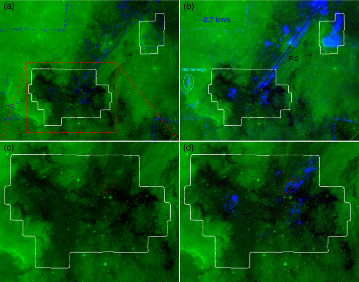
Figure B2. As B1, but at a velocity representative of F-2.
Download figure:
Standard image High-resolution imageSimilarly to F-1, the F-2 filament is in the foreground of, and has a blueshifted velocity with respect to, W80. Given the similar low extinction (i.e., being a gray region, rather than a dark region, in the optical image), and its close position and velocity relative to F-1, we argue that F-2 (similarly to F-1) is also close to the front end of the H ii region. However, since we do not see the prominent bright rims or clear feedback features in F-2 that we find in F-1, we suspect that F-2 is farther from the bubble than F-1.
Other interesting features seen at Vlsr = −2.7 km s−1 include the gas associated with the Pelican Head bright-rim region (toward the northwest) and a bright-rim region in the east, which we name Boomerang3 (see Figures 11 and B2(b)). These two mark the outer regions clearly impacted by UV radiation, and the H ii region within the DLH14 maps. Even though these features appear to be at (or close to) the edge of the H ii region, they are most likely to be in the foreground of W80, given that there is evident (light gray) extinction next to these bright-rim regions in the optical images (see Figures 1 and 11).
The above analyses of the F-1 and F-2 filaments indicates that the L935 dark cloud in the NAP region is the shadow of a combination of foreground molecular filaments and clouds. The F-3 filament identified by Z14, and shown in Figure B3 at Vlsr = 0 km s−1, appears to be part of the same complex as F-1 and F-2. As shown in Figure B3, filament F-3 winds its way from the Gulf region, through the Atlantic region, and all the way to the northern end of the Pelican region, coincident with the gray regions found in the optical images.
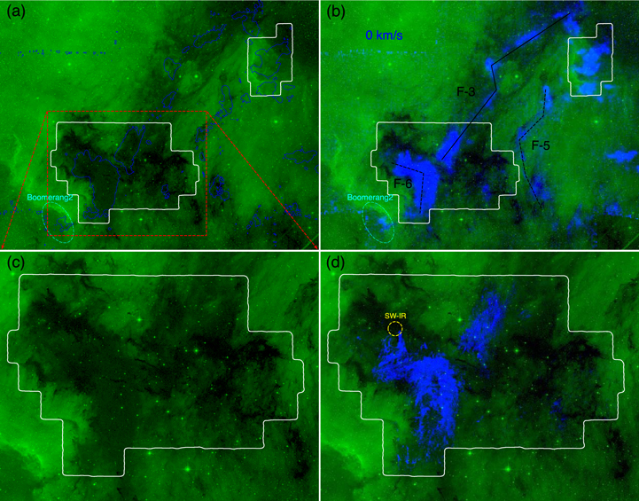
Figure B3. As B1, but at a velocity representative of F-3, F-5, and F-6.
Download figure:
Standard image High-resolution imageTwo other prominent features can be seen at velocities similar to those of F-3 (Figure B3). One of these is a filament lying on the west side of the L935 dark cloud, which follows a grayish silhouette in the optical image, and which we name F-5, following the nomenclature of Z14. The other feature is a thick filament with an “inverted L” morphology in the Gulf region. This filament, which we name F-6, corresponds to the 24 μm dark region in Figure 5, and includes the BGPS dust-continuum clumps SW1, SW2 main, SW2 SE, and SW2 S, as identified by B14 (which we show in Figure 6), as well as many 24 μm sources, and 3 YSO clusters identified by R11. Figure B3 shows that the optical counterpart of F-6 is a grayish region, similar in appearance to the optical counterparts of F-1, F-2, F-3. This region is clearly in the foreground of W80, but has not (yet) been severely impacted by the massive star. Other features seen at Vlsr ∼ 0 km s−1 include the CO emission associated with Boomerang2 in the southeast edge of the NAP complex, as well as parts of the Pelican region. As with similar features discussed above, these structures are most likely in the foreground in relation to W80.
Figure B4 shows a comparison between molecular gas at Vlsr = 1.5 km s−1 and the optical image. At this velocity, the most prominent feature is gas associated with the F-6 filament described above (also seen at Vlsr = 0 km s−1). In addition, at this velocity there are two interesting structures constituting a good match between the morphology of the CO and the gray extinction in the optical image. One is the Boomerang1 feature, shown in Figure 11 as a gray feature (see also Figure 5), where the 13CO emission nicely matches the morphology of the feedback structure. There is also a good match between the optical and the molecular gas images southwest of Boomerang1. The other structure is the silhouette highlighted by the cyan ellipse in Figure B4, at the northern edge of the Gulf region covered by our CARMA observations. As with the other features described above, the clear correspondence between gas morphology and gray extinction implies that these features are foregrounded in relation to the H ii region. Since their LSR velocity is lower than the aforementioned W80 velocity (∼5.5 km s−1), they are likely to be moving away from the bubble.
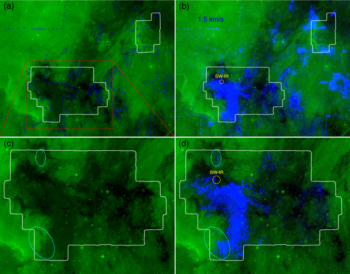
Figure B4. As B1, but at a velocity representative of F-6 and Boomerang1.
Download figure:
Standard image High-resolution imageThe molecular gas counterparts of the dark extinction regions begin to appear at higher LSR velocities. Figure B5 shows a comparison between the 13CO emission at Vlsr = 3.5 km s−1 and the optical image. The dark area in the Gulf region marked by the big dashed (cyan) circle (which we name “Dark Heron”) nicely matches the molecular gas structure. The structure extends beyond the southwestern border of our CARMA coverage, where we see the CO emission (from the DLH14-only data) matching the dark structure that we name “Dark Tail.” Another intriguing structure can be seen at the center of the Gulf region, highlighted by a dashed ellipse in panels (c) and (d) of Figure B5. It is a thin dark filament that can only be seen in the high-resolution combined data (hereafter, we name it “Dark Filigree 1”). Another dashed circle in this figure marks the structure we name the “SW-Clump,” which is to the east of the SW2 Main and SW2 SE dust-continuum clumps identified by B14. This structure appears as a darker region on top of, but with a moderately distinct velocity component in 13CO gas compared to, the gray F-6 filament. It is therefore unclear whether or not it is part of F-6 (see Section 4.2). At the northeast corner of the Gulf region we see the “Dark Worm” at the border of the CARMA mosaic footprint. We see its bottom half in the combined image, which matches well with the dark filament in the optical image.
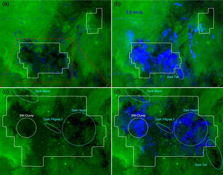
Figure B5. As B1, but at a velocity representative of the dark clumps.
Download figure:
Standard image High-resolution imageIt is evident that these dark features constitute foreground molecular gas; given their LSR velocity compared to that of W80, they are moving away from the H ii region. Unlike many of the structures coincident with the gray extinction regions, the structures at this velocity do not show clear evidence of being impacted by feedback from the high-mass star powering the H ii region. This, together with the higher extinction, causes us to infer that the dark regions are farther from the bubble as compared to the gray regions.
At Vlsr = 3.5 km s−1 we also detect emission from filament F-4, originally defined by Z14 (see Figure B5). This CO structure does not show any gray or dark counterpart in the optical image. Since it shows no optical extinction counterparts, the filament is very likely positioned on the back side of the bubble. There is another clump to the northeast of the Gulf white boundary. It shows no foreground extinction. As such, it should also be located on the far side. Its velocity peaks at roughly 4 km s−1.
Figure B6 shows a comparison between the optical image and the 13CO emission at Vlsr = 4.9 km s−1. At this velocity, a significant fraction of the molecular gas is coincident with “dark” regions that are significantly smaller than the filaments discussed above, and have the appearance of scattered clumps and drizzles, shielding light from W80 in the background. We define four structures, based on where the CO morphology at this velocity matches that of the dark regions: the “Dark Crab,” “Boomerang4,” “Dark Filigree 2,” and “Dark Drizzle.” One interesting feature is that the “Dark Drizzle” and “Dark Filigree 2” structures are broken into small dark globules, each globule having its own 13CO counterpart. The typical angular size of the globules is about 10″–15″. At a distance of 800 pc (see Section 4.3), their physical size is ∼104 au, reminiscent of Bok globules (e.g., Barnard 68, Alves et al. 2001). The Dark Crab approximately coincides in position with F-6, but is at a higher velocity. We therefore argue that the Dark Crab is in front of F-6, with a velocity similar to that of W80.
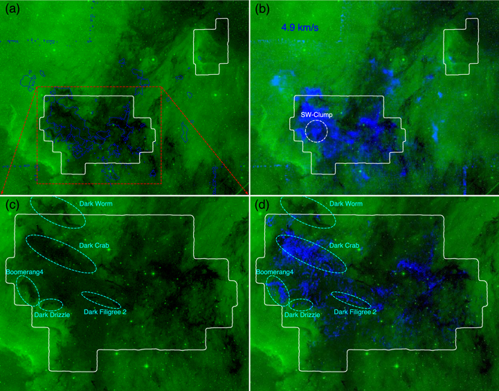
Figure B6. As B1, but at a velocity representative of the dark clumps.
Download figure:
Standard image High-resolution imageAt a Vlsr = 6.5 km s−1, there are two main structures in the 13CO emission (see Figure B7). One of these structures is associated with the Dark Crab, which we first identified when comparing the optical image of the Gulf region with the 13CO emission at Vlsr = 4.9 km s−1 (Figure B6). At Vlsr = 6.5 km s−1, most of the CO emission is concentrated toward the northeast half of the Dark Crab, whereas at lower LSR velocity, the emission associated with the Dark Crab covers the full extent of this dark cloud. The other structure at Vlsr = 6.5 km s−1, which we name F-7, lies in the southern part of the Gulf region, and is elongated in the northeast–southwest direction. Unlike other CO structures identified above, the morphology of F-7 does not closely match the structure of any of gray or dark extinction features with which it overlaps. We therefore argue that F-7 is not responsible for any of the extinction in the region, as it is located on the far side of W80. Given the LSR velocity of F-7, it is likely that F-7 is moving away from W80 (see Section 5.1 and Figure 17).
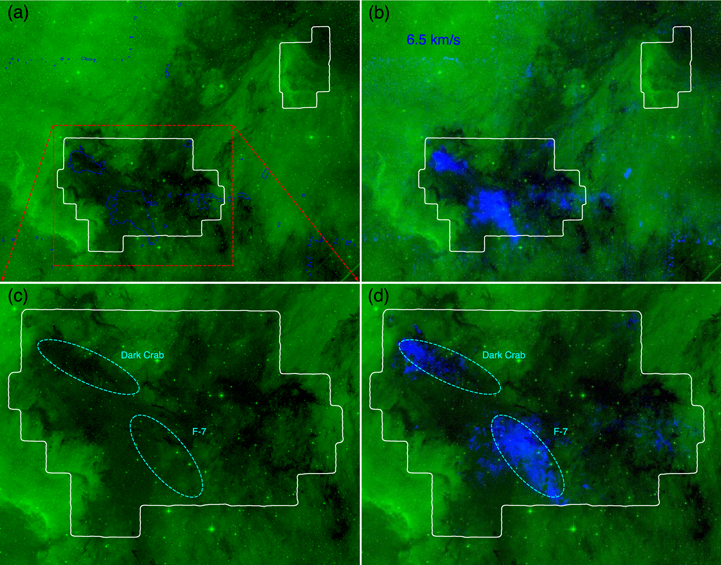
Figure B7. As B1, but at a velocity representative of F-7.
Download figure:
Standard image High-resolution imageFootnotes
- 19
In contrast to the mathematically correct covariance, we do not subtract the mean values prior to the multiplication of both maps, so as to focus on emission only.
- 20
See Fang et al. (2020) for the latest spectroscopic study of young stars in the NAP.